Downloaded 259 times


![Prim’s Algorithm
A = ø
foreach v V:
KEY[v] = ∞
PARENT[v] = null
KEY[r] = 0
Q = V
While Q != ø:
u = min (Q) by KEY value
Q = Q – u
if PARENT(u) != null:
A = A U (u, PARENT(u))
foreach v Adj(u):
if v Q and w(u,v) < KEY[v]:
PARENT[v] = u
KEY[v] = w
Return A
a
2
c
b d
f
4
6
3
4
15
e
2
A = { }
A: is used to store all edges of the minimum
spanning tree
Initially A is empty
Eventually return A
28](https://image.slidesharecdn.com/minimumspanningtreealgorithmsbyibrahimalfayoumi-151208074026-lva1-app6891/75/Minimum-spanning-tree-algorithms-by-ibrahim_alfayoumi-28-2048.jpg)
![Prim’s Algorithm
A = ø
foreach v V:
KEY[v] = ∞
PARENT[v] = null
KEY[r] = 0
Q = V
While Q != ø:
u = min (Q) by KEY value
Q = Q – u
if PARENT(u) != null:
A = A U (u, PARENT(u))
foreach v Adj(u):
if v Q and w(u,v) < KEY[v]:
PARENT[v] = u
KEY[v] = w
Return A
a
2
c
b d
f
4
6
3
4
15
e
2
A = { }
for each vertex v of the graph, Each vertex will have
two attributes KEY and PARENT
KEY and PARENT initialized to ∞ and null Respectively
29](https://image.slidesharecdn.com/minimumspanningtreealgorithmsbyibrahimalfayoumi-151208074026-lva1-app6891/75/Minimum-spanning-tree-algorithms-by-ibrahim_alfayoumi-29-2048.jpg)
![Prim’s Algorithm
A = ø
foreach v V:
KEY[v] = ∞
PARENT[v] = null
KEY[r] = 0
Q = V
While Q != ø:
u = min (Q) by KEY value
Q = Q – u
if PARENT(u) != null:
A = A U (u, PARENT(u))
foreach v Adj(u):
if v Q and w(u,v) < KEY[v]:
PARENT[v] = u
KEY[v] = w
Return A
a
2
c
b d
f
4
6
3
4
15
e
2
A = { }
for each vertex v of the graph, Each vertex will have
two attributes KEY and PARENT
KEY and PARENT initialized to ∞ and null Respectively
∞,null
∞,null
∞,null
∞,null
∞,null
∞,null
30](https://image.slidesharecdn.com/minimumspanningtreealgorithmsbyibrahimalfayoumi-151208074026-lva1-app6891/75/Minimum-spanning-tree-algorithms-by-ibrahim_alfayoumi-30-2048.jpg)
![Prim’s Algorithm
A = ø
foreach v V:
KEY[v] = ∞
PARENT[v] = null
KEY[r] = 0
Q = V
While Q != ø:
u = min (Q) by KEY value
Q = Q – u
if PARENT(u) != null:
A = A U (u, PARENT(u))
foreach v Adj(u):
if v Q and w(u,v) < KEY[v]:
PARENT[v] = u
KEY[v] = w
Return A
3
a
2
c
b d
f
4
6
4
15
e
2
A = { }
Randomly choose a vertex as a ROOT r and set its
KEY value to Zero
∞,null
∞,null
∞,null
∞,null
0,null
∞,null
31](https://image.slidesharecdn.com/minimumspanningtreealgorithmsbyibrahimalfayoumi-151208074026-lva1-app6891/75/Minimum-spanning-tree-algorithms-by-ibrahim_alfayoumi-31-2048.jpg)
![Prim’s Algorithm
A = ø
foreach v V:
KEY[v] = ∞
PARENT[v] = null
KEY[r] = 0
Q = V
While Q != ø:
u = min (Q) by KEY value
Q = Q – u
if PARENT(u) != null:
A = A U (u, PARENT(u))
foreach v Adj(u):
if v Q and w(u,v) < KEY[v]:
PARENT[v] = u
KEY[v] = w
Return A
3
a
2
c
b d
f
4
6
4
15
e
2
A = { }
Create Q list which contains all vertices in the graph
∞,null
∞,null
∞,null
∞,null
0,null
∞,null
Q = { a,b,c,d,e,f }
32](https://image.slidesharecdn.com/minimumspanningtreealgorithmsbyibrahimalfayoumi-151208074026-lva1-app6891/75/Minimum-spanning-tree-algorithms-by-ibrahim_alfayoumi-32-2048.jpg)
![Prim’s Algorithm
A = ø
foreach v V:
KEY[v] = ∞
PARENT[v] = null
KEY[r] = 0
Q = V
While Q != ø:
u = min (Q) by KEY value
Q = Q – u
if PARENT(u) != null:
A = A U (u, PARENT(u))
foreach v Adj(u):
if v Q and w(u,v) < KEY[v]:
PARENT[v] = u
KEY[v] = w
Return A
3
a
2
c
b d
f
4
6
4
15
e
2
A = { }
Find Q with the smallest (Minimum) KEY
In this case, KEY[a] = 0 (Minimum KEY)
∞,null
∞,null
∞,null
∞,null
0,null
∞,null
Q = { a,b,c,d,e,f }
33](https://image.slidesharecdn.com/minimumspanningtreealgorithmsbyibrahimalfayoumi-151208074026-lva1-app6891/75/Minimum-spanning-tree-algorithms-by-ibrahim_alfayoumi-33-2048.jpg)
![Prim’s Algorithm
A = ø
foreach v V:
KEY[v] = ∞
PARENT[v] = null
KEY[r] = 0
Q = V
While Q != ø:
u = min (Q) by KEY value
Q = Q – u
if PARENT(u) != null:
A = A U (u, PARENT(u))
foreach v Adj(u):
if v Q and w(u,v) < KEY[v]:
PARENT[v] = u
KEY[v] = w
Return A
3
a
2
c
b d
f
4
6
4
15
e
2
A = { }
Remove a from Q
∞,null
∞,null
∞,null
∞,null
0,null
∞,null
Q = { b,c,d,e,f }
34](https://image.slidesharecdn.com/minimumspanningtreealgorithmsbyibrahimalfayoumi-151208074026-lva1-app6891/75/Minimum-spanning-tree-algorithms-by-ibrahim_alfayoumi-34-2048.jpg)
![Prim’s Algorithm
A = ø
foreach v V:
KEY[v] = ∞
PARENT[v] = null
KEY[r] = 0
Q = V
While Q != ø:
u = min (Q) by KEY value
Q = Q – u
if PARENT(u) != null:
A = A U (u, PARENT(u))
foreach v Adj(u):
if v Q and w(u,v) < KEY[v]:
PARENT[v] = u
KEY[v] = w
Return A
3
a
2
c
b d
f
4
6
4
15
e
2
A = { }
PARENT [a] = null !!
Skip the if statement
∞,null
∞,null
∞,null
∞,null
0,null
∞,null
Q = { b,c,d,e,f }
35](https://image.slidesharecdn.com/minimumspanningtreealgorithmsbyibrahimalfayoumi-151208074026-lva1-app6891/75/Minimum-spanning-tree-algorithms-by-ibrahim_alfayoumi-35-2048.jpg)
![Prim’s Algorithm
A = ø
foreach v V:
KEY[v] = ∞
PARENT[v] = null
KEY[r] = 0
Q = V
While Q != ø:
u = min (Q) by KEY value
Q = Q – u
if PARENT(u) != null:
A = A U (u, PARENT(u))
foreach v Adj(u):
if v Q and w(u,v) < KEY[v]:
PARENT[v] = u
KEY[v] = w
Return A
3
a
2
c
b d
f
4
6
4
15
e
2
A = { }
Update attributes for all vertices Adjacent to a which
are b and f
Starting with f , 2 < ∞
∞,null
∞,null
∞,null
∞,null
0,null
∞,null
Q = { b,c,d,e,f }
36](https://image.slidesharecdn.com/minimumspanningtreealgorithmsbyibrahimalfayoumi-151208074026-lva1-app6891/75/Minimum-spanning-tree-algorithms-by-ibrahim_alfayoumi-36-2048.jpg)
![Prim’s Algorithm
A = ø
foreach v V:
KEY[v] = ∞
PARENT[v] = null
KEY[r] = 0
Q = V
While Q != ø:
u = min (Q) by KEY value
Q = Q – u
if PARENT(u) != null:
A = A U (u, PARENT(u))
foreach v Adj(u):
if v Q and w(u,v) < KEY[v]:
PARENT[v] = u
KEY[v] = w
Return A
3
a
2
c
b d
f
4
6
4
15
e
2
A = { }
Update attributes for all vertices Adjacent to a which are b
and f
Starting with f , 2 < ∞
PARENT [ f ] = a and KEY [ f ] = 2
∞,null
∞,null
∞,null
2, a
0,null
4, a
Q = { b,c,d,e,f }
37](https://image.slidesharecdn.com/minimumspanningtreealgorithmsbyibrahimalfayoumi-151208074026-lva1-app6891/75/Minimum-spanning-tree-algorithms-by-ibrahim_alfayoumi-37-2048.jpg)
![Prim’s Algorithm
A = ø
foreach v V:
KEY[v] = ∞
PARENT[v] = null
KEY[r] = 0
Q = V
While Q != ø:
u = min (Q) by KEY value
Q = Q – u
if PARENT(u) != null:
A = A U (u, PARENT(u))
foreach v Adj(u):
if v Q and w(u,v) < KEY[v]:
PARENT[v] = u
KEY[v] = w
Return A
3
a
2
c
b d
f
4
6
4
15
e
2
A = { (a,f) }
Now, Enter the Second Loop
a ! Q
u = min(Q) = f , Remove f from Q
PARENT [ f ] ! = null, push (a,f) to A
∞,null
∞,null
∞,null
2, a
0,null
4, a
Q = { b,c,d,e }
38](https://image.slidesharecdn.com/minimumspanningtreealgorithmsbyibrahimalfayoumi-151208074026-lva1-app6891/75/Minimum-spanning-tree-algorithms-by-ibrahim_alfayoumi-38-2048.jpg)
![Prim’s Algorithm
A = ø
foreach v V:
KEY[v] = ∞
PARENT[v] = null
KEY[r] = 0
Q = V
While Q != ø:
u = min (Q) by KEY value
Q = Q – u
if PARENT(u) != null:
A = A U (u, PARENT(u))
foreach v Adj(u):
if v Q and w(u,v) < KEY[v]:
PARENT[v] = u
KEY[v] = w
Return A
3
a
2
c
b d
f
4
6
4
15
e
2
A = { (a,f) }
Update attributes for all vertices Adjacent to f which
are c and d where weight < KEY
1, f
∞,null
4, f
2, a
0,null
4, a
Q = { b,c,d,e }
39](https://image.slidesharecdn.com/minimumspanningtreealgorithmsbyibrahimalfayoumi-151208074026-lva1-app6891/75/Minimum-spanning-tree-algorithms-by-ibrahim_alfayoumi-39-2048.jpg)
![Prim’s Algorithm
A = ø
foreach v V:
KEY[v] = ∞
PARENT[v] = null
KEY[r] = 0
Q = V
While Q != ø:
u = min (Q) by KEY value
Q = Q – u
if PARENT(u) != null:
A = A U (u, PARENT(u))
foreach v Adj(u):
if v Q and w(u,v) < KEY[v]:
PARENT[v] = u
KEY[v] = w
Return A
3
a
2
c
b d
f
4
6
4
15
e
2
A = { (a,f), (c,f) }
Now, Enter the NEXT Loop
u = min(Q) = c , Remove c from Q
PARENT [ c ] ! = null, push (c,f) to A
1, f
∞,null
4, f
2, a
0,null
4, a
Q = { b,d,e }
40](https://image.slidesharecdn.com/minimumspanningtreealgorithmsbyibrahimalfayoumi-151208074026-lva1-app6891/75/Minimum-spanning-tree-algorithms-by-ibrahim_alfayoumi-40-2048.jpg)
![Prim’s Algorithm
A = ø
foreach v V:
KEY[v] = ∞
PARENT[v] = null
KEY[r] = 0
Q = V
While Q != ø:
u = min (Q) by KEY value
Q = Q – u
if PARENT(u) != null:
A = A U (u, PARENT(u))
foreach v Adj(u):
if v Q and w(u,v) < KEY[v]:
PARENT[v] = u
KEY[v] = w
Return A
3
a
2
c
b d
f
4
6
4
15
e
2
A = { (a,f), (c,f) }
Update attributes for all vertices Adjacent to c where
weight < KEY
1, f
3, c
4, f
2, a
0,null
4, a
Q = { b,d,e }
41](https://image.slidesharecdn.com/minimumspanningtreealgorithmsbyibrahimalfayoumi-151208074026-lva1-app6891/75/Minimum-spanning-tree-algorithms-by-ibrahim_alfayoumi-41-2048.jpg)
![Prim’s Algorithm
A = ø
foreach v V:
KEY[v] = ∞
PARENT[v] = null
KEY[r] = 0
Q = V
While Q != ø:
u = min (Q) by KEY value
Q = Q – u
if PARENT(u) != null:
A = A U (u, PARENT(u))
foreach v Adj(u):
if v Q and w(u,v) < KEY[v]:
PARENT[v] = u
KEY[v] = w
Return A
3
a
2
c
b d
f
4
6
4
15
e
2
A = { (a,f), (c,f), (c,d) }
Enter the NEXT Loop
u = min(Q) = d , Remove d from Q
PARENT [ d ] ! = null, push (c,d) to A
1, f
3, c
4, f
2, a
0,null
4, a
Q = { b,e }
42](https://image.slidesharecdn.com/minimumspanningtreealgorithmsbyibrahimalfayoumi-151208074026-lva1-app6891/75/Minimum-spanning-tree-algorithms-by-ibrahim_alfayoumi-42-2048.jpg)
![Prim’s Algorithm
A = ø
foreach v V:
KEY[v] = ∞
PARENT[v] = null
KEY[r] = 0
Q = V
While Q != ø:
u = min (Q) by KEY value
Q = Q – u
if PARENT(u) != null:
A = A U (u, PARENT(u))
foreach v Adj(u):
if v Q and w(u,v) < KEY[v]:
PARENT[v] = u
KEY[v] = w
Return A
3
a
2
c
b d
f
4
6
4
15
e
2
A = { (a,f), (c,f), (c,d) }
Update attributes for all vertices Adjacent to d where
weight < KEY
1, f
3, c
2, d
2, a
0,null
4, a
Q = { b,e }
43](https://image.slidesharecdn.com/minimumspanningtreealgorithmsbyibrahimalfayoumi-151208074026-lva1-app6891/75/Minimum-spanning-tree-algorithms-by-ibrahim_alfayoumi-43-2048.jpg)
![Prim’s Algorithm
A = ø
foreach v V:
KEY[v] = ∞
PARENT[v] = null
KEY[r] = 0
Q = V
While Q != ø:
u = min (Q) by KEY value
Q = Q – u
if PARENT(u) != null:
A = A U (u, PARENT(u))
foreach v Adj(u):
if v Q and w(u,v) < KEY[v]:
PARENT[v] = u
KEY[v] = w
Return A
3
a
2
c
b d
f
4
6
4
15
e
2
A = { (a,f), (c,f), (c,d), (d,e) }
Enter the NEXT Loop
u = min(Q) = e , Remove e from Q
PARENT [ e] ! = null, push (d,e) to A
1, f
3, c
2, d
2, a
0,null
4, a
Q = { b }
44](https://image.slidesharecdn.com/minimumspanningtreealgorithmsbyibrahimalfayoumi-151208074026-lva1-app6891/75/Minimum-spanning-tree-algorithms-by-ibrahim_alfayoumi-44-2048.jpg)
![Prim’s Algorithm
A = ø
foreach v V:
KEY[v] = ∞
PARENT[v] = null
KEY[r] = 0
Q = V
While Q != ø:
u = min (Q) by KEY value
Q = Q – u
if PARENT(u) != null:
A = A U (u, PARENT(u))
foreach v Adj(u):
if v Q and w(u,v) < KEY[v]:
PARENT[v] = u
KEY[v] = w
Return A
3
a
2
c
b d
f
4
6
4
15
e
2
A = { (a,f), (c,f), (c,d), (d,e) }
No Updates for attributes because d and f ! Q
1, f
3, c
2, d
2, a
0,null
4, a
Q = { b }
45](https://image.slidesharecdn.com/minimumspanningtreealgorithmsbyibrahimalfayoumi-151208074026-lva1-app6891/75/Minimum-spanning-tree-algorithms-by-ibrahim_alfayoumi-45-2048.jpg)
![Prim’s Algorithm
A = ø
foreach v V:
KEY[v] = ∞
PARENT[v] = null
KEY[r] = 0
Q = V
While Q != ø:
u = min (Q) by KEY value
Q = Q – u
if PARENT(u) != null:
A = A U (u, PARENT(u))
foreach v Adj(u):
if v Q and w(u,v) < KEY[v]:
PARENT[v] = u
KEY[v] = w
Return A
3
a
2
c
b d
f
4
6
4
15
e
2
A = { (a,f), (c,f), (c,d), (d,e), (a,b) }
Enter the NEXT Loop
u = b , Remove b from Q
PARENT [ b] ! = null, push (a,b) to A
1, f
3, c
2, d
2, a
0,null
4, a
Q = { }
46](https://image.slidesharecdn.com/minimumspanningtreealgorithmsbyibrahimalfayoumi-151208074026-lva1-app6891/75/Minimum-spanning-tree-algorithms-by-ibrahim_alfayoumi-46-2048.jpg)
![Prim’s Algorithm
A = ø
foreach v V:
KEY[v] = ∞
PARENT[v] = null
KEY[r] = 0
Q = V
While Q != ø:
u = min (Q) by KEY value
Q = Q – u
if PARENT(u) != null:
A = A U (u, PARENT(u))
foreach v Adj(u):
if v Q and w(u,v) < KEY[v]:
PARENT[v] = u
KEY[v] = w
Return A
3
a
2
c
b d
f
4
6
4
15
e
2
A = { (a,f), (c,f), (c,d), (d,e), (a,b) }
No Updates for attributes because all neighbors of b
doesn’t exist in Q
1, f
3, c
2, d
2, a
0,null
4, a
Q = { }
47](https://image.slidesharecdn.com/minimumspanningtreealgorithmsbyibrahimalfayoumi-151208074026-lva1-app6891/75/Minimum-spanning-tree-algorithms-by-ibrahim_alfayoumi-47-2048.jpg)
![Prim’s Algorithm
A = ø
foreach v V:
KEY[v] = ∞
PARENT[v] = null
KEY[r] = 0
Q = V
While Q != ø:
u = min (Q) by KEY value
Q = Q – u
if PARENT(u) != null:
A = A U (u, PARENT(u))
foreach v Adj(u):
if v Q and w(u,v) < KEY[v]:
PARENT[v] = u
KEY[v] = w
Return A
3
a
2
c
b d
f
4
6
4
15
e
2
A = { (a,f), (c,f), (c,d), (d,e), (a,b) }
Enter the NEXT Loop, Q = ø
Exit loop
Return A
Q = { }
48](https://image.slidesharecdn.com/minimumspanningtreealgorithmsbyibrahimalfayoumi-151208074026-lva1-app6891/75/Minimum-spanning-tree-algorithms-by-ibrahim_alfayoumi-48-2048.jpg)
![Prim’s Algorithm
A = ø
foreach v V:
KEY[v] = ∞
PARENT[v] = null
KEY[r] = 0
Q = V
While Q != ø:
u = min (Q) by KEY value
Q = Q – u
if PARENT(u) != null:
A = A U (u, PARENT(u))
foreach v Adj(u):
if v Q and w(u,v) < KEY[v]:
PARENT[v] = u
KEY[v] = w
Return A
3
a
2
c
b d
f
4
6
4
15
e
2
A = { (a,f), (c,f), (c,d), (d,e), (a,b) }
Now we have a Spanning Tree that connects all
vertices which have the minimum total weight
Q = { }
49](https://image.slidesharecdn.com/minimumspanningtreealgorithmsbyibrahimalfayoumi-151208074026-lva1-app6891/75/Minimum-spanning-tree-algorithms-by-ibrahim_alfayoumi-49-2048.jpg)


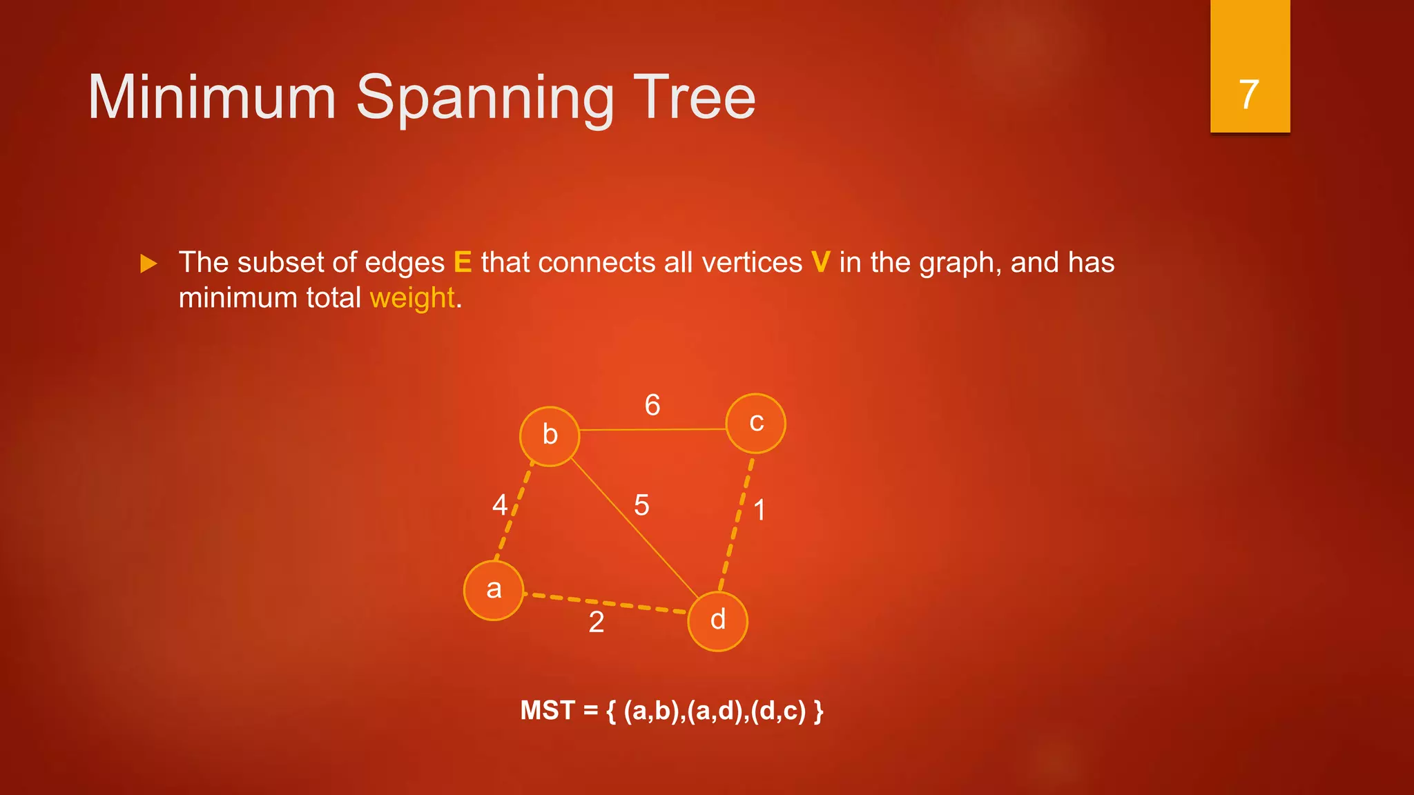
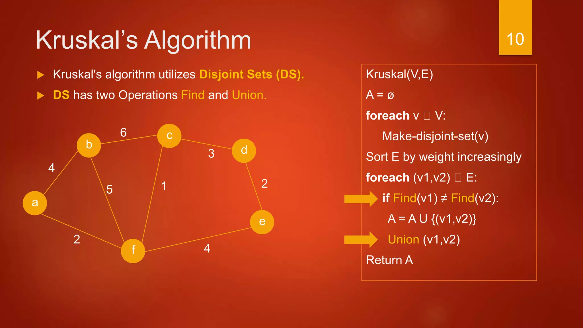
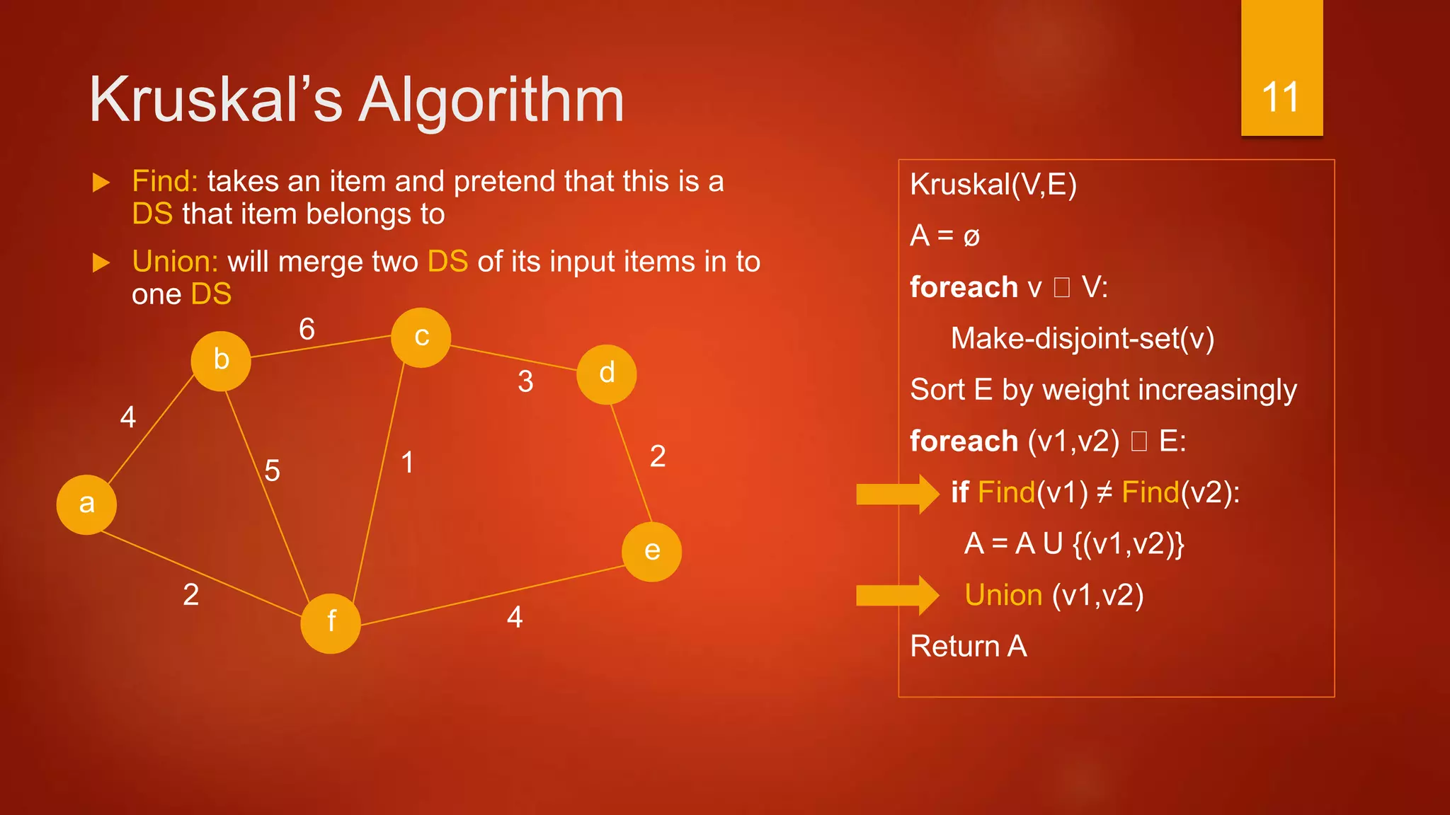
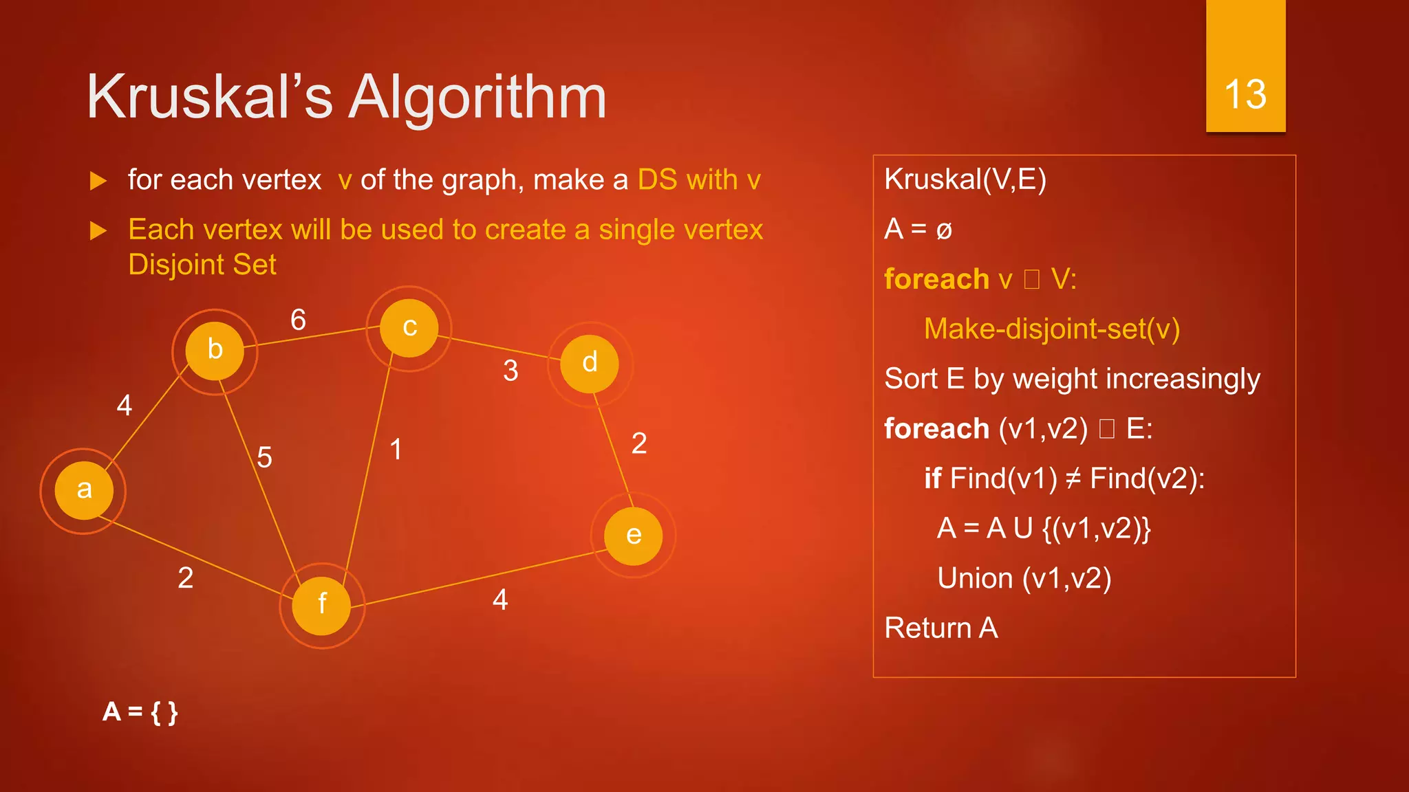
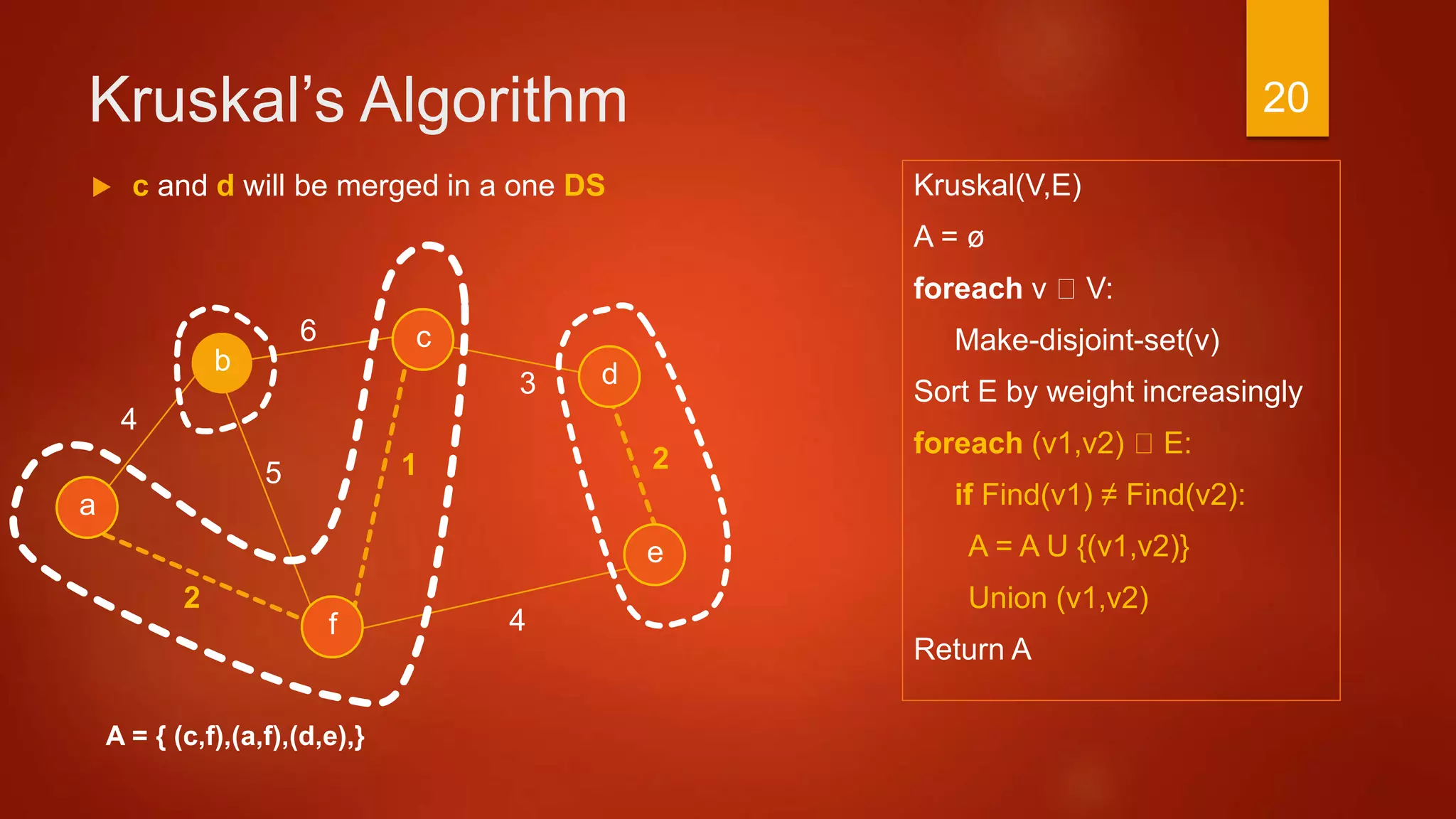
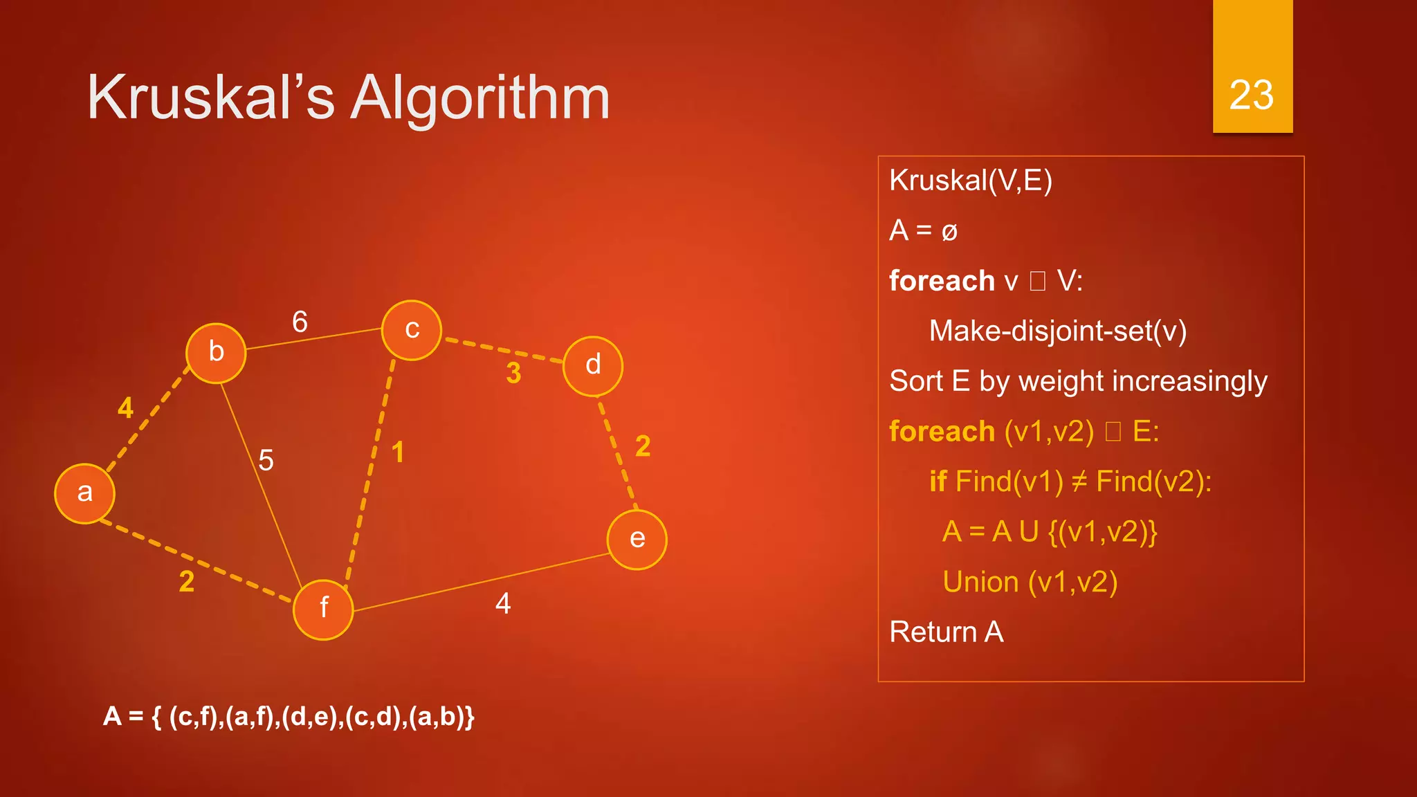
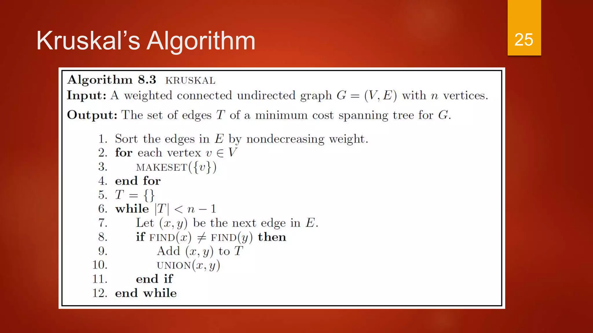
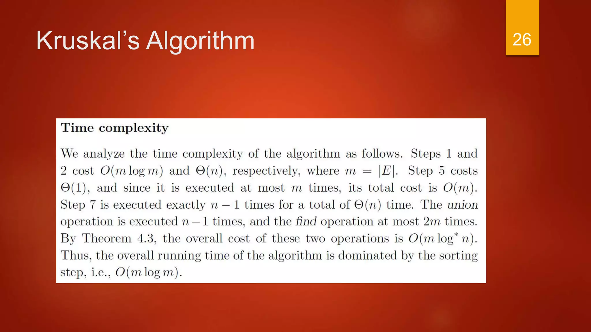
The document discusses methods for finding minimum spanning trees in graphs, focusing on Kruskal's and Prim's algorithms. It provides detailed explanations of the algorithms, including steps and operations involved in constructing the trees while ensuring minimal total weight. The document illustrates these concepts with examples and pseudo-code to enhance understanding.