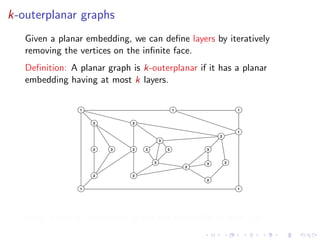
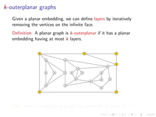
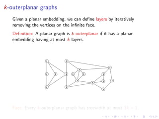
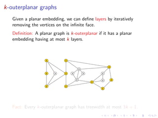
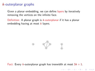
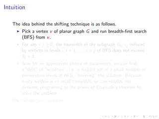
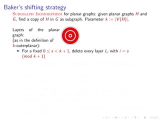
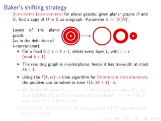
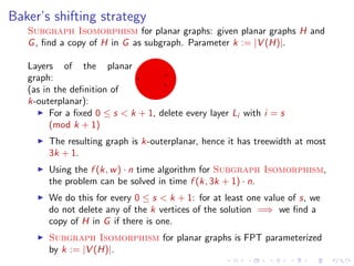
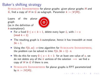
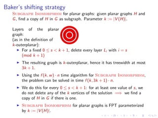
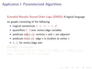
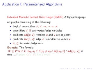
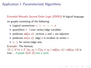
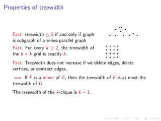
The document discusses applications of graphs with bounded treewidth. It covers the following key points:
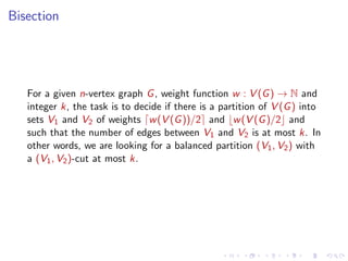
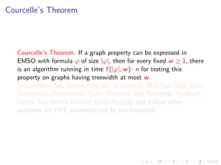
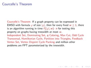
1) Courcelle's theorem shows that many NP-complete graph problems can be solved in linear time for graphs of bounded treewidth using monadic second-order logic. This includes problems like independent set, coloring, and Hamiltonian cycle.
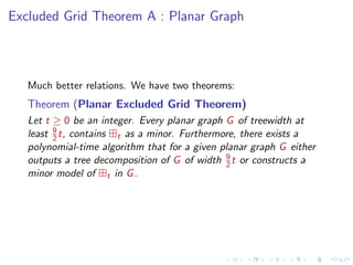
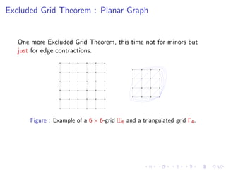
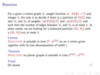
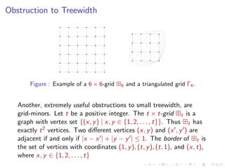
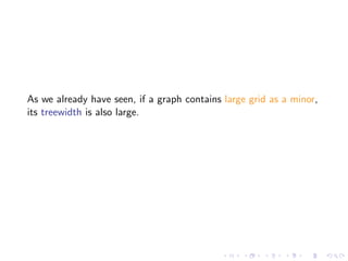
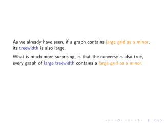
2) The treewidth of a graph is closely related to its largest grid minor - graphs with large treewidth contain large grid minors. There are polynomial relationships between treewidth and largest grid minor for planar graphs.
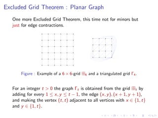
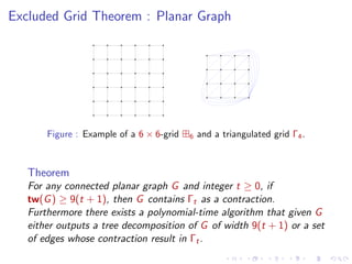
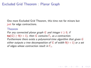
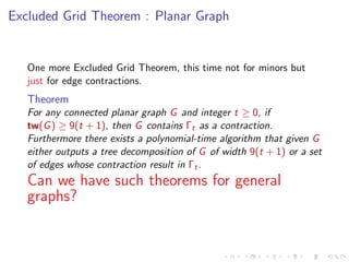
3) Planar graphs have bounded treewidth if and only if they exclude some grid configuration as a contraction. This helps characterize planar graphs of bounded treewidth
![Excluded Grid Theorem
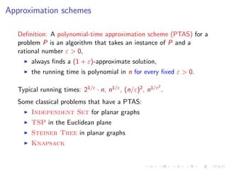
Fact: [Excluded Grid Theorem] If the treewidth of G is at least
2
k 4k (k+2) , then G has a k × k grid minor.
[Robertson and Seymour ]](https://image.slidesharecdn.com/slidesapplicationsoftreewidth-140307123730-phpapp01/85/Treewidth-and-Applications-16-320.jpg)
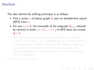
![Excluded Grid Theorem
Fact: [Excluded Grid Theorem] If the treewidth of G is at least
2
k 4k (k+2) , then G has a k × k grid minor.
[Robertson and Seymour ]
It was open for many years whether a polynomial relationship could
be established between the treewidth of a graph G and the size of
its largest grid minor.](https://image.slidesharecdn.com/slidesapplicationsoftreewidth-140307123730-phpapp01/85/Treewidth-and-Applications-17-320.jpg)
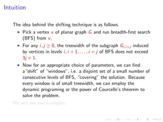
![Excluded Grid Theorem
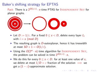
Fact: [Excluded Grid Theorem] If the treewidth of G is at least
2
k 4k (k+2) , then G has a k × k grid minor.
[Robertson and Seymour ]
It was open for many years whether a polynomial relationship could
be established between the treewidth of a graph G and the size of
its largest grid minor.
Theorem (Excluded Grid Theorem, Chekuri and Chuzhoy)
Let t ≥ 0 be an integer. There exists a universal constant c, such
that every graph of treewidth at least c · t 99 contains t as a
minor.](https://image.slidesharecdn.com/slidesapplicationsoftreewidth-140307123730-phpapp01/85/Treewidth-and-Applications-18-320.jpg)
![Excluded Grid Theorem
Fact: [Excluded Grid Theorem] If the treewidth of G is at least
2
k 4k (k+2) , then G has a k × k grid minor.
[Robertson and Seymour ]](https://image.slidesharecdn.com/slidesapplicationsoftreewidth-140307123730-phpapp01/85/Treewidth-and-Applications-19-320.jpg)
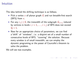
![Excluded Grid Theorem
Fact: [Excluded Grid Theorem] If the treewidth of G is at least
2
k 4k (k+2) , then G has a k × k grid minor.
[Robertson and Seymour ]
It was open for many years whether a polynomial relationship could
be established between the treewidth of a graph G and the size of
its largest grid minor.](https://image.slidesharecdn.com/slidesapplicationsoftreewidth-140307123730-phpapp01/85/Treewidth-and-Applications-20-320.jpg)
![Excluded Grid Theorem
Fact: [Excluded Grid Theorem] If the treewidth of G is at least
2
k 4k (k+2) , then G has a k × k grid minor.
[Robertson and Seymour ]
It was open for many years whether a polynomial relationship could
be established between the treewidth of a graph G and the size of
its largest grid minor.
Theorem (Excluded Grid Theorem, Chekuri and Chuzhoy)
Let t ≥ 0 be an integer. There exists a universal constant c, such
that every graph of treewidth at least c · t 99 contains t as a
minor.](https://image.slidesharecdn.com/slidesapplicationsoftreewidth-140307123730-phpapp01/85/Treewidth-and-Applications-21-320.jpg)