Topological sorting

Dr. AMIT KUMAR @JUET
Graph Algorithms – 2

graphs-2 - 2 Lin / DeviDr. AMIT KUMAR @JUET
Identification of Edges
 Edge type for edge (u, v) can be identified when it is first explored
by DFS.
 Identification is based on the color of v.
» White – tree edge.
» Gray – back edge.
» Black – forward or cross edge.

Directed Acyclic Graph
 DAG – Directed graph with no cycles.
 Good for modeling processes and structures that have a
partial order:
» a > b and b > c  a > c.
» But may have a and b such that neither a > b nor b > a.
 Can always make a total order (either a > b or b > a for
all a  b) from a partial order.

Example
DAG of dependencies for putting on goalie equipment.
socks shorts
hose
pants
skates
leg pads
T-shirt
chest pad
sweater
mask
catch glove
blocker
batting glove

Characterizing a DAG
Proof:
 : Show that back edge  cycle.
» Suppose there is a back edge (u, v). Then v is ancestor of u in
depth-first forest.
» Therefore, there is a path v u, so v u v is a cycle.
Lemma 22.11
A directed graph G is acyclic iff a DFS of G yields no back edges.
v u
T T T
B

Characterizing a DAG
Proof (Contd.):
  : Show that a cycle implies a back edge.
» c : cycle in G, v : first vertex discovered in c, (u, v) : preceding
edge in c.
» At time d[v], vertices of c form a white path v u. Why?
» By white-path theorem, u is a descendent of v in depth-first
forest.
» Therefore, (u, v) is a back edge.
Lemma 22.11
A directed graph G is acyclic iff a DFS of G yields no back edges.
v u
T T T
B

Topological Sort
Want to “sort” a directed acyclic graph (DAG).
B
E
D
C
A
C EDA B
Think of original DAG as a partial order.
Want a total order that extends this partial order.

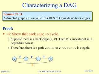
Topological Sort
 Performed on a DAG.
 Linear ordering of the vertices of G such that if (u, v) 
E, then u appears somewhere before v.
Topological-Sort (G)
1. call DFS(G) to compute finishing times f [v] for all v  V
2. as each vertex is finished, insert it onto the front of a linked list
3. return the linked list of vertices
Time: (V + E).
Example: On board.

Example
Linked List:
A B D
C E
1/
(Courtesy of Prof. Jim Anderson)

Example
Linked List:
A B D
C E
1/
2/

Example
Linked List:
A B D
C E
1/
2/3
E
2/3

Example
Linked List:
A B D
C E
1/4
2/3
E
2/31/4
D

Example
Linked List:
A B D
C E
1/4
2/3
E
2/31/4
D
5/

Example
Linked List:
A B D
C E
1/4
2/3
E
2/31/4
D
5/
6/

Example
Linked List:
A B D
C E
1/4
2/3
E
2/31/4
D
5/
6/7
6/7
C

Example
Linked List:
A B D
C E
1/4
2/3
E
2/31/4
D
5/8
6/7
6/7
C
5/8
B

Example
Linked List:
A B D
C E
1/4
2/3
E
2/31/4
D
5/8
6/7
6/7
C
5/8
B
9/

Example
Linked List:
A B D
C E
1/4
2/3
E
2/31/4
D
5/8
6/7
6/7
C
5/8
B
9/10
9/10
A

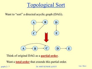
Correctness Proof
 Just need to show if (u, v)  E, then f [v] < f [u].
 When we explore (u, v), what are the colors of u and v?
» u is gray.
» Is v gray, too?
• No, because then v would be ancestor of u.
•  (u, v) is a back edge.
•  contradiction of Lemma 22.11 (dag has no back edges).
» Is v white?
• Then becomes descendant of u.
• By parenthesis theorem, d[u] < d[v] < f [v] < f [u].
» Is v black?
• Then v is already finished.
• Since we’re exploring (u, v), we have not yet finished u.
• Therefore, f [v] < f [u].

Strongly Connected Components
 G is strongly connected if every pair (u, v) of vertices in
G is reachable from one another.
 A strongly connected component (SCC) of G is a
maximal set of vertices C  V such that for all u, v  C,
both u v and v u exist.

Component Graph
 GSCC = (VSCC, ESCC).
 VSCC has one vertex for each SCC in G.
 ESCC has an edge if there’s an edge between the
corresponding SCC’s in G.
 GSCC for the example considered:

GSCC is a DAG
Proof:
 Suppose there is a path v v in G.
 Then there are paths u u v and v v u in G.
 Therefore, u and v are reachable from each other, so they
are not in separate SCC’s.
Lemma 22.13
Let C and C be distinct SCC’s in G, let u, v  C, u, v  C, and
suppose there is a path u u in G. Then there cannot also be a path
v v in G.

Transpose of a Directed Graph
 GT = transpose of directed G.
» GT = (V, ET), ET = {(u, v) : (v, u)  E}.
» GT is G with all edges reversed.
 Can create GT in Θ(V + E) time if using adjacency lists.
 G and GT have the same SCC’s. (u and v are reachable
from each other in G if and only if reachable from each
other in GT.)

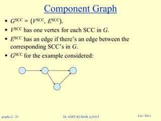
Algorithm to determine SCCs
SCC(G)
1. call DFS(G) to compute finishing times f [u] for all u
2. compute GT
3. call DFS(GT), but in the main loop, consider vertices in order of
decreasing f [u] (as computed in first DFS)
4. output the vertices in each tree of the depth-first forest formed in
second DFS as a separate SCC
Time: (V + E).
Example: On board.

Example
13/14
12/15 3/4 2/7
11/16 1/10
a b c
e f g
5/6
8/9
h
d
(Courtesy of Prof. Jim Anderson)
G

Example
a b c
e f g h
d
GT

Example
cd
hfg
abe

How does it work?
 Idea:
» By considering vertices in second DFS in decreasing order of
finishing times from first DFS, we are visiting vertices of the
component graph in topologically sorted order.
» Because we are running DFS on GT, we will not be visiting any
v from a u, where v and u are in different components.
 Notation:
» d[u] and f [u] always refer to first DFS.
» Extend notation for d and f to sets of vertices U  V:
» d(U) = minuU{d[u]} (earliest discovery time)
» f (U) = maxuU{ f [u]} (latest finishing time)

SCCs and DFS finishing times
Proof:
 Case 1: d(C) < d(C)
» Let x be the first vertex discovered in C.
» At time d[x], all vertices in C and C are
white. Thus, there exist paths of white
vertices from x to all vertices in C and C.
» By the white-path theorem, all vertices in
C and C are descendants of x in depth-
first tree.
» By the parenthesis theorem, f [x] = f (C)
> f(C).
Lemma 22.14
Let C and C be distinct SCC’s in G = (V, E). Suppose there is an
edge (u, v)  E such that u  C and v C. Then f (C) > f (C).
C C
u v
x

Proof:
 Case 2: d(C) > d(C)
» Let y be the first vertex discovered in C.
» At time d[y], all vertices in C are white and
there is a white path from y to each vertex in
C  all vertices in C become descendants
of y. Again, f [y] = f (C).
» At time d[y], all vertices in C are also white.
» By earlier lemma, since there is an edge (u,
v), we cannot have a path from C to C.
» So no vertex in C is reachable from y.
» Therefore, at time f [y], all vertices in C are
still white.
» Therefore, for all w  C, f [w] > f [y], which
implies that f (C) > f (C).
Lemma 22.14
edge (u, v)  E such that u  C and v C. Then f (C) > f (C).
C C
u v
yx

Proof:
 (u, v)  ET  (v, u)  E.
 Since SCC’s of G and GT are the same, f(C) > f (C), by
Lemma 22.14.
Corollary 22.15
edge
(u, v)  ET, where u  C and v  C. Then f(C) < f(C).

Correctness of SCC
 When we do the second DFS, on GT, start with SCC C
such that f(C) is maximum.
» The second DFS starts from some x  C, and it visits all
vertices in C.
» Corollary 22.15 says that since f(C) > f (C) for all C  C, there
are no edges from C to C in GT.
» Therefore, DFS will visit only vertices in C.
» Which means that the depth-first tree rooted at x contains
exactly the vertices of C.

Correctness of SCC
 The next root chosen in the second DFS is in SCC C
such that f (C) is maximum over all SCC’s other than C.
» DFS visits all vertices in C, but the only edges out of C go to
C, which we’ve already visited.
» Therefore, the only tree edges will be to vertices in C.
 We can continue the process.
 Each time we choose a root for the second DFS, it can
reach only
» vertices in its SCC—get tree edges to these,
» vertices in SCC’s already visited in second DFS—get no tree
edges to these.

Topological sorting

More Related Content

What's hot

Similar to Topological sorting

More from Amit Kumar Rathi

Recently uploaded

Topological sorting