Downloaded 69 times
![CHAPTER 4
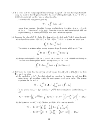
4.1. The value of E at P(ρ = 2, φ = 40◦
, z = 3) is given as E = 100aρ − 200aφ + 300az V/m.
Determine the incremental work required to move a 20 µC charge a distance of 6 µm:
a) in the direction of aρ: The incremental work is given by dW = −q E · dL, where in this
case, dL = dρ aρ = 6 × 10⁻⁶
aρ. Thus
dW = −(20 × 10−6
C)(100 V/m)(6 × 10−6
m) = −12 × 10−9
J = −12 nJ
b) in the direction of aφ: In this case dL = 2 dφ aφ = 6 × 10⁻⁶
aφ, and so
dW = −(20 × 10−6
)(−200)(6 × 10⁻⁶
) = 2.4 × 10⁻⁸
J = 24 nJ
c) in the direction of az: Here, dL = dz az = 6 × 10⁻⁶
az, and so
dW = −(20 × 10−6
)(300)(6 × 10⁻⁶
) = −3.6 × 10⁻⁸
J = −36 nJ
d) in the direction of E: Here, dL = 6 × 10⁻⁶
aE, where
aE =
100aρ − 200aφ + 300az
[1002 + 2002 + 3002]1/2
= 0.267 aρ − 0.535 aφ + 0.802 az
Thus
dW = −(20 × 10−6
)[100aρ − 200aφ + 300az] · [0.267 aρ − 0.535 aφ + 0.802 az](6 × 10⁻⁶
)
= −44.9 nJ
e) In the direction of G = 2 ax − 3 ay + 4 az: In this case, dL = 6 × 10⁻⁶
aG, where
aG =
2ax − 3ay + 4az
[22 + 32 + 42]1/2
= 0.371 ax − 0.557 ay + 0.743 az
So now
dW = −(20 × 10−6
)[100aρ − 200aφ + 300az] · [0.371 ax − 0.557 ay + 0.743 az](6 × 10⁻⁶
)
= −(20 × 10−6
) [37.1(aρ · ax) − 55.7(aρ · ay) − 74.2(aφ · ax) + 111.4(aφ · ay)
+ 222.9] (6 × 10⁻⁶
)
where, at P, (aρ · ax) = (aφ · ay) = cos(40◦
) = 0.766, (aρ · ay) = sin(40◦
) = 0.643, and
(aφ · ax) = − sin(40◦
) = −0.643. Substituting these results in
dW = −(20 × 10−6
)[28.4 − 35.8 + 47.7 + 85.3 + 222.9](6 × 10⁻⁶
) = −41.8 nJ
42](https://image.slidesharecdn.com/capitulo47ed-140509155200-phpapp01/85/Capitulo-4-7ma-edicion-1-320.jpg)
![CHAPTER 4
4.1. The value of E at P(ρ = 2, φ = 40◦
, z = 3) is given as E = 100aρ − 200aφ + 300az V/m.
Determine the incremental work required to move a 20 µC charge a distance of 6 µm:
a) in the direction of aρ: The incremental work is given by dW = −q E · dL, where in this
case, dL = dρ aρ = 6 × 10⁻⁶
aρ. Thus
dW = −(20 × 10−6
C)(100 V/m)(6 × 10−6
m) = −12 × 10−9
J = −12 nJ
b) in the direction of aφ: In this case dL = 2 dφ aφ = 6 × 10⁻⁶
aφ, and so
dW = −(20 × 10−6
)(−200)(6 × 10⁻⁶
) = 2.4 × 10⁻⁸
J = 24 nJ
c) in the direction of az: Here, dL = dz az = 6 × 10⁻⁶
az, and so
dW = −(20 × 10−6
)(300)(6 × 10⁻⁶
) = −3.6 × 10⁻⁸
J = −36 nJ
d) in the direction of E: Here, dL = 6 × 10⁻⁶
aE, where
aE =
100aρ − 200aφ + 300az
[1002 + 2002 + 3002]1/2
= 0.267 aρ − 0.535 aφ + 0.802 az
Thus
dW = −(20 × 10−6
)[100aρ − 200aφ + 300az] · [0.267 aρ − 0.535 aφ + 0.802 az](6 × 10⁻⁶
)
= −44.9 nJ
e) In the direction of G = 2 ax − 3 ay + 4 az: In this case, dL = 6 × 10⁻⁶
aG, where
aG =
2ax − 3ay + 4az
[22 + 32 + 42]1/2
= 0.371 ax − 0.557 ay + 0.743 az
So now
dW = −(20 × 10−6
)[100aρ − 200aφ + 300az] · [0.371 ax − 0.557 ay + 0.743 az](6 × 10⁻⁶
)
= −(20 × 10−6
) [37.1(aρ · ax) − 55.7(aρ · ay) − 74.2(aφ · ax) + 111.4(aφ · ay)
+ 222.9] (6 × 10⁻⁶
)
where, at P, (aρ · ax) = (aφ · ay) = cos(40◦
) = 0.766, (aρ · ay) = sin(40◦
) = 0.643, and
(aφ · ax) = − sin(40◦
) = −0.643. Substituting these results in
dW = −(20 × 10−6
)[28.4 − 35.8 + 47.7 + 85.3 + 222.9](6 × 10⁻⁶
) = −41.8 nJ
42](https://image.slidesharecdn.com/capitulo47ed-140509155200-phpapp01/75/Capitulo-4-7ma-edicion-1-2048.jpg)
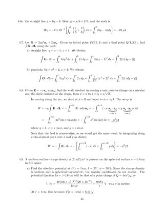
![4.2. An electric field is given as E = −10ey
(sin 2z ax + x sin 2z ay + 2x cos 2z az) V/m.
a) Find E at P(5, 0, π/12): Substituting this point into the given field produces
EP = −10 [sin(π/6) ax + 5 sin(π/6) ay + 10 cos(π/6) az] = − 5 ax + 25 ay + 50
√
3 az
b) How much work is done in moving a charge of 2 nC an incremental distance of 1 mm
from P in the direction of ax? This will be
dWx = −qE · dL ax = −2 × 10⁻⁹
(−5)(10−3
) = 10−11
J = 10 pJ
c) of ay?
dWy = −qE · dL ay = −2 × 10⁻⁹
(−25)(10−3
) = 50−11
J = 50 pJ
d) of az?
dWz = −qE · dL az = −2 × 10⁻⁹
(−50
√
3)(10−3
) = 100
√
3 pJ
e) of (ax + ay + az)?
dWxyz = −qE · dL
ax + ay + az)
√
3
=
10 + 50 + 100
√
3
√
3
= 135 pJ
4.3. If E = 120 aρ V/m, find the incremental amount of work done in moving a 50 µm charge a
distance of 2 mm from:
a) P(1, 2, 3) toward Q(2, 1, 4): The vector along this direction will be Q − P = (1, −1, 1)
from which aP Q = [ax − ay + az]/
√
3. We now write
dW = −qE · dL = −(50 × 10−6
) 120aρ ·
(ax − ay + az
√
3
(2 × 10⁻³
)
= −(50 × 10−6
)(120) [(aρ · ax) − (aρ · ay)]
1
√
3
(2 × 10⁻³
)
At P, φ = tan−1
(2/1) = 63.4◦
. Thus (aρ · ax) = cos(63.4) = 0.447 and (aρ · ay) =
sin(63.4) = 0.894. Substituting these, we obtain dW = 3.1 µJ.
b) Q(2, 1, 4) toward P(1, 2, 3): A little thought is in order here: Note that the field has only
a radial component and does not depend on φ or z. Note also that P and Q are at the
same radius (
√
5) from the z axis, but have different φ and z coordinates. We could just
as well position the two points at the same z location and the problem would not change.
If this were so, then moving along a straight line between P and Q would thus involve
moving along a chord of a circle whose radius is
√
5. Halfway along this line is a point of
symmetry in the field (make a sketch to see this). This means that when starting from
either point, the initial force will be the same. Thus the answer is dW = 3.1 µJ as in part
a. This is also found by going through the same procedure as in part a, but with the
direction (roles of P and Q) reversed.
43](https://image.slidesharecdn.com/capitulo47ed-140509155200-phpapp01/85/Capitulo-4-7ma-edicion-2-320.jpg)
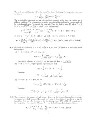
![b) Find VAB given points A(r = 2 cm, θ = 30◦
, φ = 60◦
) and B(r = 3 cm, θ = 45◦
, φ = 90◦
):
Again, the angles do not matter because of the spherical symmetry. We use the part a
result to obtain
VAB = VA − VB = 0.081
1
0.02
−
1
0.03
= 1.36 V
4.10. Express the potential field of an infinite line charge
a) with zero reference at ρ = ρ0: We write in general:
V (ρ) = −
ρL
2π 0ρ
dρ + C1 = −
ρL
2π 0
ln(ρ) + C1 = 0 at ρ = ρ0
Therefore
C1 =
ρL
2π 0
ln(ρ0)
and finally
V (ρ) =
ρL
2π 0
[ln(ρ0) − ln(ρ)] =
ρL
2π 0
ln
ρ0
ρ
b) with V = V0 at ρ = ρ0: Using the reasoning of part a, we have
V (ρ0) = V0 =
ρL
2π 0
ln(ρ0) + C2 ⇒ C2 = V0 +
ρL
2π 0
ln(ρ0)
and finally
V (ρ) =
ρL
2π 0
ln
ρ0
ρ
+ V0
c) Can the zero reference be placed at infinity? Why? Answer: No, because we would have
a potential that is proportional to the undefined ln(∞/ρ).
4.11. Let a uniform surface charge density of 5 nC/m2
be present at the z = 0 plane, a uniform line
charge density of 8 nC/m be located at x = 0, z = 4, and a point charge of 2 µC be present
at P(2, 0, 0). If V = 0 at M(0, 0, 5), find V at N(1, 2, 3): We need to find a potential function
for the combined charges which is zero at M. That for the point charge we know to be
Vp(r) =
Q
4π 0r
Potential functions for the sheet and line charges can be found by taking indefinite integrals
of the electric fields for those distributions. For the line charge, we have
Vl(ρ) = −
ρl
2π 0ρ
dρ + C1 = −
ρl
2π 0
ln(ρ) + C1
For the sheet charge, we have
Vs(z) = −
ρs
2 0
dz + C2 = −
ρs
2 0
z + C2
46](https://image.slidesharecdn.com/capitulo47ed-140509155200-phpapp01/85/Capitulo-4-7ma-edicion-5-320.jpg)
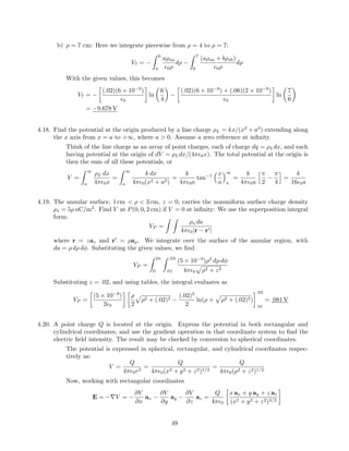
![4.14. Given the electric field E = (y + 1)ax + (x − 1)ay + 2az, find the potential difference between
the points
a) (2,-2,-1) and (0,0,0): We choose a path along which motion occurs in one coordinate
direction at a time. Starting at the origin, first move along x from 0 to 2, where y = 0;
then along y from 0 to −2, where x is 2; then along z from 0 to −1. The setup is
Vb − Va = −
2
0
(y + 1)
y=0
dx −
−2
0
(x − 1)
x=2
dy −
−1
0
2 dz = 2
b) (3,2,-1) and (-2,-3,4): Following similar reasoning,
Vb − Va = −
3
−2
(y + 1)
y=−3
dx −
2
−3
(x − 1)
x=3
dy −
−1
4
2 dz = 10
4.15. Two uniform line charges, 8 nC/m each, are located at x = 1, z = 2, and at x = −1, y = 2
in free space. If the potential at the origin is 100 V, find V at P(4, 1, 3): The net potential
function for the two charges would in general be:
V = −
ρl
2π 0
ln(R1) −
ρl
2π 0
ln(R2) + C
At the origin, R1 = R2 =
√
5, and V = 100 V. Thus, with ρl = 8 × 10⁻⁹
,
100 = −2
(8 × 10⁻⁹
)
2π 0
ln(
√
5) + C ⇒ C = 331.6 V
At P(4, 1, 3), R1 = |(4, 1, 3)−(1, 1, 2)| =
√
10 and R2 = |(4, 1, 3)−(−1, 2, 3)| =
√
26. Therefore
VP = −
(8 × 10⁻⁹
)
2π 0
ln(
√
10) + ln(
√
26) + 331.6 = −68.4 V
4.16. The potential at any point in space is given in cylindrical coordinates by V = (k/ρ2
) cos(bφ)
V/m, where k and b are constants.
a) Where is the zero reference for potential? This will occur at ρ → ∞, or whenever
cos(bφ) = 0, which gives φ = (2m − 1)π/2b, where m = 1, 2, 3...
b) Find the vector electric field intensity at any point (ρ, φ, z). We use
E(ρ, φ, z) = −∇V = −
∂V
∂ρ
aρ −
1
ρ
∂V
∂φ
aφ =
k
ρ3
[2 cos(bφ) aρ + b sin(bφ) aφ]
4.17. Uniform surface charge densities of 6 and 2 nC/m2
are present at ρ = 2 and 6 cm respectively,
in free space. Assume V = 0 at ρ = 4 cm, and calculate V at:
a) ρ = 5 cm: Since V = 0 at 4 cm, the potential at 5 cm will be the potential difference
between points 5 and 4:
V5 = −
5
4
E · dL = −
5
4
aρsa
0ρ
dρ = −
(.02)(6 × 10⁻⁹
)
0
ln
5
4
= −3.026 V
48](https://image.slidesharecdn.com/capitulo47ed-140509155200-phpapp01/85/Capitulo-4-7ma-edicion-7-320.jpg)
![4.21d) |E|P : taking the magnitude of the part c result, we find |E|P = 75.0 V/m.
e) aN : By definition, this will be
aN
P
= −
E
|E|
= −0.095 ax − 0.304 ay + 0.948 az
f) D: This is D
P
= 0E
P
= 62.8 ax + 202 ay − 629 az pC/m2
.
4.22. A certain potential field is given in spherical coordinates by V = V0(r/a) sin θ. Find the total
charge contained within the region r < a: We first find the electric field through
E = −∇V = −
∂V
∂r
ar −
1
r
∂V
∂θ
= −
V0
a
[sin θ ar + cos θ aθ]
The requested charge is now the net outward flux of D = 0E through the spherical shell of
radius a (with outward normal ar):
Q =
S
D · dS =
2π
0
π
0
0E · ar a2
sin θ dθ dφ = −2πaV0 0
π
0
sin2
θ dθ = −π2
a 0V0 C
The same result can be found (as expected) by taking the divergence of D and integrating
over the spherical volume:
∇ · D = −
1
r2
∂
∂r
r2 0V0
a
sin θ −
1
r sin θ
∂
∂θ
0V0
a
cos θ sin θ = −
0V0
ra
2 sin θ +
cos(2θ)
sin θ
= −
0V0
ra sin θ
2 sin2
θ + 1 − 2 sin2
θ =
− 0V0
ra sin θ
= ρv
Now
Q =
2π
0
π
0
a
0
− 0V0
ra sin θ
r2
sin θ dr dθ dφ =
−2π2
0V0
a
a
0
r dr = −π2
a 0V0 C
4.23. It is known that the potential is given as V = 80ρ.6
V. Assuming free space conditions, find:
a) E: We find this through
E = −∇V = −
dV
dρ
aρ = −48ρ−.4
V/m
b) the volume charge density at ρ = .5 m: Using D = 0E, we find the charge density
through
ρv
.5
= [∇ · D].5 =
1
ρ
d
dρ
(ρDρ)
.5
= −28.8 0ρ−1.4
.5
= −673 pC/m3
c) the total charge lying within the closed surface ρ = .6, 0 < z < 1: The easiest way to do
this calculation is to evaluate Dρ at ρ = .6 (noting that it is constant), and then multiply
51](https://image.slidesharecdn.com/capitulo47ed-140509155200-phpapp01/85/Capitulo-4-7ma-edicion-10-320.jpg)
![by the cylinder area: Using part a, we have Dρ
.6
= −48 0(.6)−.4
= −521 pC/m2
. Thus
Q = −2π(.6)(1)521 × 10−12
C = −1.96 nC.
4.24. The surface defined by the equation x3
+ y2
+ z = 1000, where x, y, and z are positive, is an
equipotential surface on which the potential is 200 V. If |E| = 50 V/m at the point P(7, 25, 32)
on the surface, find E there:
First, the potential function will be of the form V (x, y, z) = C1(x3
+ y2
+ z) + C2, where
C1 and C2 are constants to be determined (C2 is in fact irrelevant for our purposes). The
electric field is now
E = −∇V = −C1(3x2
ax + 2y ay + az)
And the magnitude of E is |E| = C1 9x4 + 4y2 + 1, which at the given point will be
|E|P = C1 9(7)4 + 4(25)2 + 1 = 155.27C1 = 50 ⇒ C1 = 0.322
Now substitute C1 and the given point into the expression for E to obtain
EP = −(47.34 ax + 16.10 ay + 0.32 az)
The other constant, C2, is needed to assure a potential of 200 V at the given point.
4.25. Within the cylinder ρ = 2, 0 < z < 1, the potential is given by V = 100 + 50ρ + 150ρ sin φ V.
a) Find V , E, D, and ρv at P(1, 60◦
, 0.5) in free space: First, substituting the given point,
we find VP = 279.9 V. Then,
E = −∇V = −
∂V
∂ρ
aρ −
1
ρ
∂V
∂φ
aφ = − [50 + 150 sin φ] aρ − [150 cos φ] aφ
Evaluate the above at P to find EP = −179.9aρ − 75.0aφ V/m
Now D = 0E, so DP = −1.59aρ − .664aφ nC/m2
. Then
ρv = ∇·D =
1
ρ
d
dρ
(ρDρ)+
1
ρ
∂Dφ
∂φ
= −
1
ρ
(50 + 150 sin φ) +
1
ρ
150 sin φ 0 = −
50
ρ
0 C
At P, this is ρvP = −443 pC/m3
.
b) How much charge lies within the cylinder? We will integrate ρv over the volume to obtain:
Q =
1
0
2π
0
2
0
−
50 0
ρ
ρ dρ dφ dz = −2π(50) 0(2) = −5.56 nC
52](https://image.slidesharecdn.com/capitulo47ed-140509155200-phpapp01/85/Capitulo-4-7ma-edicion-11-320.jpg)
![4.26. Let us assume that we have a very thin, square, imperfectly conducting plate 2m on a side,
located in the plane z = 0 with one corner at the origin such that it lies entirely within the
first quadrant. The potential at any point in the plate is given as V = −e−x
sin y.
a) An electron enters the plate at x = 0, y = π/3 with zero initial velocity; in what direction
is its initial movement? We first find the electric field associated with the given potential:
E = −∇V = −e−x
[sin y ax − cos y ay]
Since we have an electron, its motion is opposite that of the field, so the direction on
entry is that of −E at (0, π/3), or
√
3/2 ax − 1/2 ay.
b) Because of collisions with the particles in the plate, the electron achieves a relatively low
velocity and little acceleration (the work that the field does on it is converted largely into
heat). The electron therefore moves approximately along a streamline. Where does it
leave the plate and in what direction is it moving at the time? Considering the result
of part a, we would expect the exit to occur along the bottom edge of the plate. The
equation of the streamline is found through
Ey
Ex
=
dy
dx
= −
cos y
sin y
⇒ x = − tan y dy + C = ln(cos y) + C
At the entry point (0, π/3), we have 0 = ln[cos(π/3)] + C, from which C = 0.69. Now,
along the bottom edge (y = 0), we find x = 0.69, and so the exit point is (0.69, 0). From
the field expression evaluated at the exit point, we find the direction on exit to be −ay.
4.27. Two point charges, 1 nC at (0, 0, 0.1) and −1 nC at (0, 0, −0.1), are in free space.
a) Calculate V at P(0.3, 0, 0.4): Use
VP =
q
4π 0|R+|
−
q
4π 0|R−|
where R+
= (.3, 0, .3) and R−
= (.3, 0, .5), so that |R+
| = 0.424 and |R−
| = 0.583. Thus
VP =
10−9
4π 0
1
.424
−
1
.583
= 5.78 V
b) Calculate |E| at P: Use
EP =
q(.3ax + .3az)
4π 0(.424)3
−
q(.3ax + .5az)
4π 0(.583)3
=
10−9
4π 0
[2.42ax + 1.41az] V/m
Taking the magnitude of the above, we find |EP | = 25.2 V/m.
c) Now treat the two charges as a dipole at the origin and find V at P: In spherical coor-
dinates, P is located at r =
√
.32 + .42 = .5 and θ = sin−1
(.3/.5) = 36.9◦
. Assuming a
dipole in far-field, we have
VP =
qd cos θ
4π 0r2
=
10−9
(.2) cos(36.9◦
)
4π 0(.5)2
= 5.76 V
53](https://image.slidesharecdn.com/capitulo47ed-140509155200-phpapp01/85/Capitulo-4-7ma-edicion-12-320.jpg)
![4.28. Use the electric field intensity of the dipole (Sec. 4.7, Eq. (36)) to find the difference in
potential between points at θa and θb, each point having the same r and φ coordinates. Under
what conditions does the answer agree with Eq. (34), for the potential at θa?
We perform a line integral of Eq. (36) along an arc of constant r and φ:
Vab = −
θa
θb
qd
4π 0r3
[2 cos θ ar + sin θ aθ] · aθ r dθ = −
θa
θb
qd
4π 0r2
sin θ dθ
=
qd
4π 0r2
[cos θa − cos θb]
This result agrees with Eq. (34) if θa (the ending point in the path) is 90◦
(the xy plane).
Under this condition, we note that if θb > 90◦
, positive work is done when moving (against
the field) to the xy plane; if θb < 90◦
, negative work is done since we move with the field.
4.29. A dipole having a moment p = 3ax −5ay +10az nC · m is located at Q(1, 2, −4) in free space.
Find V at P(2, 3, 4): We use the general expression for the potential in the far field:
V =
p · (r − r )
4π 0|r − r |3
where r − r = P − Q = (1, 1, 8). So
VP =
(3ax − 5ay + 10az) · (ax + ay + 8az) × 10−9
4π 0[12 + 12 + 82]1.5
= 1.31 V
4.30. A dipole for which p = 10 0 az C · m is located at the origin. What is the equation of the
surface on which Ez = 0 but E = 0?
First we find the z component:
Ez = E · az =
10
4πr3
[2 cos θ (ar · az) + sin θ (aθ · az)] =
5
2πr3
2 cos2
θ − sin2
θ
This will be zero when 2 cos2
θ − sin2
θ = 0. Using identities, we write
2 cos2
θ − sin2
θ =
1
2
[1 + 3 cos(2θ)]
The above becomes zero on the cone surfaces, θ = 54.7◦
and θ = 125.3◦
.
4.31. A potential field in free space is expressed as V = 20/(xyz) V.
a) Find the total energy stored within the cube 1 < x, y, z < 2. We integrate the energy
density over the cube volume, where wE = (1/2) 0E · E, and where
E = −∇V = 20
1
x2yz
ax +
1
xy2z
ay +
1
xyz2
az V/m
The energy is now
WE = 200 0
2
1
2
1
2
1
1
x4y2z2
+
1
x2y4z2
+
1
x2y2z4
dx dy dz
54](https://image.slidesharecdn.com/capitulo47ed-140509155200-phpapp01/85/Capitulo-4-7ma-edicion-13-320.jpg)
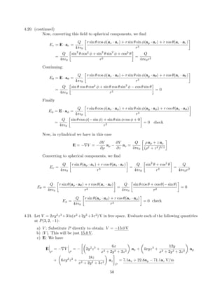
![4.31a. (continued)
The integral evaluates as follows:
WE = 200 0
2
1
2
1
−
1
3
1
x3y2z2
−
1
xy4z2
−
1
xy2z4
2
1
dy dz
= 200 0
2
1
2
1
7
24
1
y2z2
+
1
2
1
y4z2
+
1
2
1
y2z4
dy dz
= 200 0
2
1
−
7
24
1
yz2
−
1
6
1
y3z2
−
1
2
1
yz4
2
1
dz
= 200 0
2
1
7
48
1
z2
+
7
48
1
z2
+
1
4
1
z4
dz
= 200 0(3)
7
96
= 387 pJ
b) What value would be obtained by assuming a uniform energy density equal to the value
at the center of the cube? At C(1.5, 1.5, 1.5) the energy density is
wE = 200 0(3)
1
(1.5)4(1.5)2(1.5)2
= 2.07 × 10⁻¹⁰
J/m3
This, multiplied by a cube volume of 1, produces an energy value of 207 pJ.
4.32. Using Eq. (36), a) find the energy stored in the dipole field in the region r > a:
We start with
E(r, θ) =
qd
4π 0r3
[2 cos θ ar + sin θ aθ]
Then the energy will be
We =
vol
1
2
0E · E dv =
2π
0
π
0
∞
a
(qd)2
32π2
0r6
4 cos2
θ + sin2
θ
3 cos2 θ+1
r2
sin θ dr dθ dφ
=
−2π(qd)2
32π2
0
1
3r3
∞
a
π
0
3 cos2
θ + 1 sin θ dθ =
(qd)2
48π2
0a3
− cos3
θ − cos θ
π
0
4
=
(qd)2
12π 0a3
J
b) Why can we not let a approach zero as a limit? From the above result, a singularity in the
energy occurs as a → 0. More importantly, a cannot be too small, or the original far-field
assumption used to derive Eq. (36) (a >> d) will not hold, and so the field expression
will not be valid.
4.33. A copper sphere of radius 4 cm carries a uniformly-distributed total charge of 5 µC in free
space.
a) Use Gauss’ law to find D external to the sphere: with a spherical Gaussian surface at
radius r, D will be the total charge divided by the area of this sphere, and will be ar-
directed. Thus
D =
Q
4πr2
ar =
5 × 10⁻⁶
4πr2
ar C/m2
55](https://image.slidesharecdn.com/capitulo47ed-140509155200-phpapp01/85/Capitulo-4-7ma-edicion-14-320.jpg)
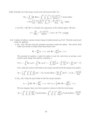

1. The document provides calculations for determining work done by electric fields on charges moving through various paths. It includes determining incremental work from given electric field expressions and calculating potentials from different charge distributions. 2. Key results include the work done on a 20 μC charge moving in different directions in a given electric field, the potential and potential difference from a uniform spherical charge distribution, and expressing the potential field of an infinite line charge with different references. 3. The final problem calculates the potential at a point from the combined electric fields of a uniform sheet charge, uniform line charge, and point charge, with the potential set to zero at a reference point.


