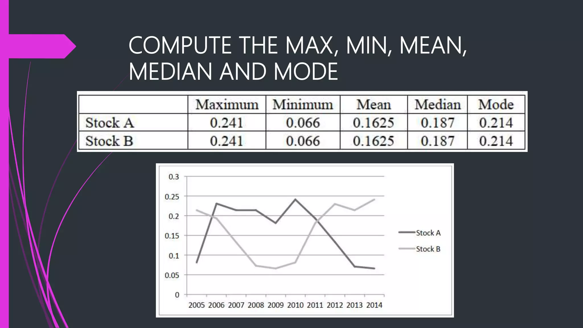
Measures of
Variation
Learning Outcomes
Calculate some measures of dispersion;
Think of the strengths and limitations of these
measures; and
Provide a sound interpretation of these
measures.
The Case of Returns on Stocks
 Stocks are shares of ownership in a company. When people
buy stocks they become part owners of the company,
whether in terms of profits or losses of the company.
RATE OF RETURN
is defined as the increase in value of the portfolio
(including any dividends or other distributions)
during the year divided by its value at the beginning
of the year.
For instance, if the parents of Juana dela Cruz
invests 50,000 pesos in a stock at the beginning of
the year, and the value of the stock goes up to
60,000 pesos, thus having an increase in value of
10,000 pesos, then the rate of return here is
10,000/50,000 = 0.20
COMPUTE THE MAX, MIN, MEAN,
MEDIAN AND MODE
Notice that there are no differences in the computed
summary statistics but the trend and actual values of
the rate of returns for the two stocks are different as
depicted in the line graph.
Such observation tells us that it is not enough to
simply use measures of location to describe a data
set. We need additional measures such as measures
of variation or dispersion to describe further the data
sets.
In particular, summary measures of variability (such
as the range and the standard deviation) of the rates
of return are used to measure risk associated with
investment.
We could use measures of variation to decide
whether it would make any difference if we
decide to invest wholly in Stock A, wholly in
Stock B, or half of our investments in Stock A
and another half in Stock B.
In general, there is higher risk in investing if
the rate of return fluctuates much or there is
high variability in its historical values. Thus, we
choose investment where the risk of the rate
of return has a small measure of dispersion.
TWO TYPES OF MEASURES OF
VARIABILITY OR DISPERSION
1. Absolute measure of dispersion provides a measure of
variability of observations or values within a data set.
includes the range, interquartile range, variance, and
standard deviation.
2. Relative measure of dispersion which is the other type of
measure of dispersion is used to compare variability of
data sets of different variables or variables measured in
different units of measurement. The coefficient of
variation is a relative measure of variability.
ABSOLUTE MEASURES
OF DISPERSION
Range, Interquartile range, Variance, and Standard
Deviation
RANGE
The range is a simple measure of variation defined
as the difference between the maximum and
minimum values.
The range depends on the extremes; it ignores
information about what goes in between the
smallest (minimum) and largest (maximum) values
in a data set.
The larger the range, the larger is the dispersion of
the data set.
WHAT IS THE RANGE?
INTERQUARTILE RANGE
The interquartile range or IQR is the difference
between the 3rd and the 1st quartiles. Hence, it
gives you the spread of the middle 50% of the data
set.
Like the range, the higher the value of the IQR, the
larger is the dispersion of the data set. Based on the
computations we did in the previous lesson, the 3rd
quartile or 𝑄3 is the 113th observation and is equal
to 38 while 𝑄1 or 𝑃25 is the 38th observation and is
equal to 25. Hence, IQR = = 38 – 25 = 13.
VARIANCE
Variance is a measure of dispersion that accounts
for the average squared deviation of each
observation from the mean.
Since we square the difference of each observation
from the mean, the unit of measurement of the
variance is the square of the unit used in measuring
each observation. Such property is a little bit
problematic in interpretation. For example, point2 or
kilogram2 is difficult to interpret compared to
inches2.
FORMULA FOR VARIANCE
𝜎2
=
𝑖=1
𝑁
𝑥𝑖 − 𝜇 2
𝑁
So what we did is for each unique observation we
subtract the mean, we refer to the difference as di,
square the difference and sum it for all
observations. Note that in the table we have to
multiply the square of the difference with the
number of students to account for all observations.
We then divide the sum by the total number of
observations, denoted by 𝑁.
Thus, in this example 𝜎2
= 14,009/150 = 93.39
STANDARD DEVIATION
Standard deviation is computed which is the
positive square of the variance, that is 𝜎 =
𝜎2.
In the example, 𝜎2
= 93.39, thus 𝜎 =
93.3933 = 9.6640.
To interpret, we say that on the average, the
scores of the students deviate from the mean
score of 32 points by as much as 9.6640 or
approximately 10 points
If all the observations are equal to a constant, then
the mean is that constant, and the measure of
variation is zero. Furthermore, if for a given data set,
the variance and standard deviation turn out to be
zero, then all the deviations from the average must
be zero, which means that all observations are equal.
Note that if a data set were rescaled, that is if the
observations were multiplied by some constant, then
the standard deviation of the new data set is merely
the scaling factor multiplied to the standard
deviation of the original data set.
The variance and standard deviation are based on all
the observations items in the data set, and each item
is given a proper weight. They are extremely useful
measures of variability as they measure the average
scattering of the data around the mean, that is how
large data fluctuate above and below the mean. The
variance and standard deviation increase with an
increase in the deviations about the mean, and
decrease with decreases in these deviations. A small
standard deviation (and variance) means a high
degree of uniformity in the observations and of
homogeneity in a series.
 The variance is the most suitable for algebraic manipulations
but as was pointed out earlier, its value is in squared unit of
measurements. On the other hand, the standard deviation
has unit of measure same as with that of the observations.
Thus, standard deviation serves as the primary measure of
variation, just as the mean is the primary measure of central
location.
 Going back to the motivation example on the stocks where
in we have two stocks, A and B. Both stocks have same
expected return measured by the mean. However, the
standard deviation of the rates of return for Stock A is 0.0688
while that for Stock B is 0.0685, indicating that Stock A has
higher risk compared to Stock B although the difference is
not that large.
RELATIVE MEASURE
OF DISPERSION
Coefficient of Variation
COEFFICIENT OF VARIATION
 To compare variability between or among different data sets,
that is, the data sets are for different variables or same
variables but measured in different unit of measurement, the
coefficient of variation (CV) is used as measure of relative
dispersion.
 It is usually expressed as percentage and is computed as
𝐶𝑉 =
𝜎
𝜇
× 100%.
 CV is a measure of dispersion relative to the mean of the
data set. With and having same unit of measurement, CV is
unit less or it does not depend on the unit of measurement.
Hence, it is used compare the variability across the different
data sets.
EXAMPLE
 The CV of the scores of the students in the long test is
computed as
𝐶𝑉 =
𝜎
𝜇
× 100% =
9.6640
32.04667
× 100% = 30.16%
 While the CV of the rate of returns of Stock A is
𝐶𝑉 =
𝜎
𝜇
× 100% =
0.0688
0.1625
× 100% = 42.34%
 Thus, we say the rate of returns of Stock A is more variable
than the scores of the students in the test. Here, we used the
CV to compare the variability of two different data sets.
KEY POINTS
Measure of dispersion is used to further describe
the distribution of the data set.
Absolute measures of variation include range,
interquartile range, variance and standard deviation.
A relative measure of dispersion is provided by the
coefficient of variation.

Measures of Variation

  • 1.
  • 2.
    Learning Outcomes Calculate somemeasures of dispersion; Think of the strengths and limitations of these measures; and Provide a sound interpretation of these measures.
  • 3.
    The Case ofReturns on Stocks  Stocks are shares of ownership in a company. When people buy stocks they become part owners of the company, whether in terms of profits or losses of the company.
  • 4.
    RATE OF RETURN isdefined as the increase in value of the portfolio (including any dividends or other distributions) during the year divided by its value at the beginning of the year. For instance, if the parents of Juana dela Cruz invests 50,000 pesos in a stock at the beginning of the year, and the value of the stock goes up to 60,000 pesos, thus having an increase in value of 10,000 pesos, then the rate of return here is 10,000/50,000 = 0.20
  • 5.
    COMPUTE THE MAX,MIN, MEAN, MEDIAN AND MODE
  • 6.
    Notice that thereare no differences in the computed summary statistics but the trend and actual values of the rate of returns for the two stocks are different as depicted in the line graph. Such observation tells us that it is not enough to simply use measures of location to describe a data set. We need additional measures such as measures of variation or dispersion to describe further the data sets. In particular, summary measures of variability (such as the range and the standard deviation) of the rates of return are used to measure risk associated with investment.
  • 7.
    We could usemeasures of variation to decide whether it would make any difference if we decide to invest wholly in Stock A, wholly in Stock B, or half of our investments in Stock A and another half in Stock B. In general, there is higher risk in investing if the rate of return fluctuates much or there is high variability in its historical values. Thus, we choose investment where the risk of the rate of return has a small measure of dispersion.
  • 8.
    TWO TYPES OFMEASURES OF VARIABILITY OR DISPERSION 1. Absolute measure of dispersion provides a measure of variability of observations or values within a data set. includes the range, interquartile range, variance, and standard deviation. 2. Relative measure of dispersion which is the other type of measure of dispersion is used to compare variability of data sets of different variables or variables measured in different units of measurement. The coefficient of variation is a relative measure of variability.
  • 9.
    ABSOLUTE MEASURES OF DISPERSION Range,Interquartile range, Variance, and Standard Deviation
  • 10.
    RANGE The range isa simple measure of variation defined as the difference between the maximum and minimum values. The range depends on the extremes; it ignores information about what goes in between the smallest (minimum) and largest (maximum) values in a data set. The larger the range, the larger is the dispersion of the data set.
  • 11.
  • 12.
    INTERQUARTILE RANGE The interquartilerange or IQR is the difference between the 3rd and the 1st quartiles. Hence, it gives you the spread of the middle 50% of the data set. Like the range, the higher the value of the IQR, the larger is the dispersion of the data set. Based on the computations we did in the previous lesson, the 3rd quartile or 𝑄3 is the 113th observation and is equal to 38 while 𝑄1 or 𝑃25 is the 38th observation and is equal to 25. Hence, IQR = = 38 – 25 = 13.
  • 13.
    VARIANCE Variance is ameasure of dispersion that accounts for the average squared deviation of each observation from the mean. Since we square the difference of each observation from the mean, the unit of measurement of the variance is the square of the unit used in measuring each observation. Such property is a little bit problematic in interpretation. For example, point2 or kilogram2 is difficult to interpret compared to inches2.
  • 14.
  • 16.
    So what wedid is for each unique observation we subtract the mean, we refer to the difference as di, square the difference and sum it for all observations. Note that in the table we have to multiply the square of the difference with the number of students to account for all observations. We then divide the sum by the total number of observations, denoted by 𝑁. Thus, in this example 𝜎2 = 14,009/150 = 93.39
  • 17.
    STANDARD DEVIATION Standard deviationis computed which is the positive square of the variance, that is 𝜎 = 𝜎2. In the example, 𝜎2 = 93.39, thus 𝜎 = 93.3933 = 9.6640. To interpret, we say that on the average, the scores of the students deviate from the mean score of 32 points by as much as 9.6640 or approximately 10 points
  • 18.
    If all theobservations are equal to a constant, then the mean is that constant, and the measure of variation is zero. Furthermore, if for a given data set, the variance and standard deviation turn out to be zero, then all the deviations from the average must be zero, which means that all observations are equal. Note that if a data set were rescaled, that is if the observations were multiplied by some constant, then the standard deviation of the new data set is merely the scaling factor multiplied to the standard deviation of the original data set.
  • 19.
    The variance andstandard deviation are based on all the observations items in the data set, and each item is given a proper weight. They are extremely useful measures of variability as they measure the average scattering of the data around the mean, that is how large data fluctuate above and below the mean. The variance and standard deviation increase with an increase in the deviations about the mean, and decrease with decreases in these deviations. A small standard deviation (and variance) means a high degree of uniformity in the observations and of homogeneity in a series.
  • 20.
     The varianceis the most suitable for algebraic manipulations but as was pointed out earlier, its value is in squared unit of measurements. On the other hand, the standard deviation has unit of measure same as with that of the observations. Thus, standard deviation serves as the primary measure of variation, just as the mean is the primary measure of central location.  Going back to the motivation example on the stocks where in we have two stocks, A and B. Both stocks have same expected return measured by the mean. However, the standard deviation of the rates of return for Stock A is 0.0688 while that for Stock B is 0.0685, indicating that Stock A has higher risk compared to Stock B although the difference is not that large.
  • 21.
  • 22.
    COEFFICIENT OF VARIATION To compare variability between or among different data sets, that is, the data sets are for different variables or same variables but measured in different unit of measurement, the coefficient of variation (CV) is used as measure of relative dispersion.  It is usually expressed as percentage and is computed as 𝐶𝑉 = 𝜎 𝜇 × 100%.  CV is a measure of dispersion relative to the mean of the data set. With and having same unit of measurement, CV is unit less or it does not depend on the unit of measurement. Hence, it is used compare the variability across the different data sets.
  • 23.
    EXAMPLE  The CVof the scores of the students in the long test is computed as 𝐶𝑉 = 𝜎 𝜇 × 100% = 9.6640 32.04667 × 100% = 30.16%  While the CV of the rate of returns of Stock A is 𝐶𝑉 = 𝜎 𝜇 × 100% = 0.0688 0.1625 × 100% = 42.34%  Thus, we say the rate of returns of Stock A is more variable than the scores of the students in the test. Here, we used the CV to compare the variability of two different data sets.
  • 24.
    KEY POINTS Measure ofdispersion is used to further describe the distribution of the data set. Absolute measures of variation include range, interquartile range, variance and standard deviation. A relative measure of dispersion is provided by the coefficient of variation.

Editor's Notes

  • #4 To introduce this lesson, tell the students the importance of thinking about their future, of saving, and of wealth generation. Explain that a number of people invest money into the stock market as an alternative financial instrument to generate wealth from savings. WRITE Mention to students that the history of performance of a particular stock maybe a useful guide to what may be expected of its performance in the foreseeable future. This is of course, a very big assumption, but we have to assume it anyway.
  • #5 Explain to students that the rate of return may be positive or negative. It represents the fraction by which your wealth would have changed had it been invested in that particular combination of securities.
  • #6 Call students. WHAT CAN YOU OBSERVE?
  • #11 We already encountered the range in previous lesson where we discussed the construction of an FDT.
  • #12 In the above data, the maximum is 50 and the minimum is 10, hence the range is 40. But note that the range could be easily affected by the values of the extremes as mentioned earlier as the range depends only on the extremities. Because of this property, another measure, the interquartile range or IQR is used instead.
  • #25 Worksheet