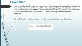
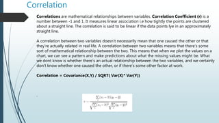
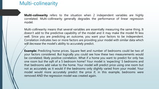
In this slide, variables types, probability theory behind the algorithms and its uses including distribution is explained. Also theorems like bayes theorem is also explained.
Intro and maths behind Bayes theorem. Bayes theorem as a classifier. NB algorithm and examples of bayes. Intro to knn algorithm, lazy learning, cosine similarity. Basics of recommendation and filtering methods.
Intro to SVM with its maths and examples. Types of SVM and its parameters. Concept of vector algebra. Concepts of text analytics and Natural Language Processing along with its applications.
Machine learning session6(decision trees random forrest)Abhimanyu Dwivedi
Concepts include decision tree with its examples. Measures used for splitting in decision tree like gini index, entropy, information gain, pros and cons, validation. Basics of random forests with its example and uses.
very detailed illustration of Log of Odds, Logit/ logistic regression and their types from binary logit, ordered logit to multinomial logit and also with their assumptions.
Thanks, for your time, if you enjoyed this short article there are tons of topics in advanced analytics, data science, and machine learning available in my medium repo. https://medium.com/@bobrupakroy
Data Science - Part III - EDA & Model SelectionDerek Kane
This lecture introduces the concept of EDA, understanding, and working with data for machine learning and predictive analysis. The lecture is designed for anyone who wants to understand how to work with data and does not get into the mathematics. We will discuss how to utilize summary statistics, diagnostic plots, data transformations, variable selection techniques including principal component analysis, and finally get into the concept of model selection.
Types of Probability Distributions - Statistics IIRupak Roy
Get to know in detail the definitions of the types of probability distributions from binomial, poison, hypergeometric, negative binomial to continuous distribution like t-distribution and much more.
Let me know if anything is required. Ping me at google #bobrupakroy
Get to know more about Directional and Non-Directional Hypothesis tests like one-tail, two-tailed along with 2 sample tests, paired difference T-test, if you are interested to implement the same in python check out my other blogs. Ping me @ google #bobrupakroy Happy Data Science Talk soon!
Multiple sample test - Anova, Chi-square, Test of association, Goodness of Fit Rupak Roy
Detailed demonstration of Multiple Sample Test like Analysis of Variance (ANOVA), kinds of ANOVA One Way, Two Way, Chi-square with their assumptions and applications using excel, and much more.
Let me know if anything is needed. Happy to help. ping @ #bobrupakroy
Data Preparation with the help of Analytics MethodologyRupak Roy
Get involved with the steps of data preparation and data assessment using widely used methodologies for machine learning data science modeling.
Let me know if anything is required, ping me at google #bobrupakroy
Linear regression is an approach for modeling the relationship between one dependent variable and one or more independent variables.
Algorithms to minimize the error are
OLS (Ordinary Least Square)
Gradient Descent and much more.
Let me know if anything is required. Ping me at google #bobrupakroy
Don't get confused with Summary Statistics. Learn in-depth types of summary statistics from measures of central tendency, measures of dispersion and much more.
Let me know if anything is required. ping me at google #bobrupakroy
Learn to perform hypothesis testing with their stages of hypothesis testing with ease with the help of Excel and much more. See ya soon. Ping @ #bobrupakroy
Machine Learning Decision Tree AlgorithmsRupak Roy
Details discussion about the Tree Algorithms like Gini, Information Gain, Chi-square for categorical and Reduction in variance for continuous variable. Let me know if anything is required. Happy to help. Enjoy machine learning! #bobrupakroy
Data Science - Part XV - MARS, Logistic Regression, & Survival AnalysisDerek Kane
This lecture provides an overview on extending the regression concepts brought forth in previous lectures. We will start off by going through a broad overview of the Multivariate Adaptive Regression Splines Algorithm, Logistic Regression, and then explore the Survival Analysis. The presentation will culminate with a real world example on how these techniques can be used in the US criminal justice system.
Statistical Inference Part II: Types of Sampling DistributionDexlab Analytics
This is an in-depth analysis of the way different types of sampling distribution works focusing on their specific functions and interrelations as part of the discussion on the theory of sampling.
This article provides a brief discussion on several statistical parameters that are most commonly used in any measurement and analysis process. There are a plethora of such parameters but the most important and widely used are briefed in here.
Guided notes covering background material on Statistics for IB Biology. This content was formerly Topic 1 but it is no longer a formal topic for the new 2016 syllabus.
Levels of Measurement: Nominal = Data one collects when doing a wide-open descriptive or exploratory study, however, it is not limited to these kinds of studies. We can count this data, but we can’t order it. We need to be able to put this data into categories that are mutually exclusive, i.e. it can’t be in more than one category at a time. An example would be looking at age, race, sex, or some other type of data that you either are or aren’t. The categories need to be exhaustive – there need to be enough categories to cover the data you collect. Ordinal = this category has mutually exclusive categories, but with ordinal data you can order the data within each category. The ratings of poor, fair, good are an example of ordinal information. Note that you can order the ratings, but you can’t really tell how far apart each of these descriptors are from each other. You could also look at who finishes a task first, second, third, and so on. Again, you can rank this data, but you don’t know how much faster the first person was in relation to the second person or subsequent people. Interval-ratio data = this type of data allows you to measure the difference between each of your rankings. Data is ordered (as with ordinal data) and you can tell how much difference there is between each observation because there is a scale that is divided into equal units. You can measure a race with a stopwatch in terms of seconds or tenths of seconds. A thermometer gives you data with measurements in degrees. Ratio data is like interval data (and is often lumped together with it because they are usually handled the same way statistically). Its primary difference is that there is a zero point on the scale so that you can do multiplication and division. Money is an example of a ratio scale – two dollars are exactly twice one dollar. Volume, area, and distance measures are also ratio scales (2 times 1 liter equals 2 liters). This is different from a strict interval scale like a thermometer – we can’t say that 10 degrees Fahrenheit is twice as warm as 5 degrees Fahrenheit. Statistical Distributions: According to Shi, “a distribution organizes the values of a variable into categories. Frequency Distribution (aka Marginal Distribution): Displays the number of cases that falls into each category. Percentage Distribution: Found by dividing the number of frequency of cases in the category by the total N. Measures of Central Tendency: Mean: The most common measure of central tendency. It simply the sum of the numbers divided by the number of numbers. Median: It is defined as the middle position or midpoint of a distribution. Mode: Is defined as the most frequently occurring value. What is variability? Amount of spread or dispersion within a distribution of scores within a set of data. Measures of Variability: Range: The difference between the highest and lowest values in a distribution. Interquartile Range: Known as the ‘midspread’ or ‘middle fifty.” It contains the middle 50% of
Segunda parte del Curso de Perfeccionamiento Profesional no Conducente a Grado Académico: Inglés Técnico para Profesionales de Ciencias de la Salud. DEPARTAMENTO ADMINISTRATIVO SOCIAL. Escuela de Enfermería. ULA. Mérida. Venezuela. Se oferta en la modalidad presencial de 3 ó 4 unidades crédito y los costos son solidarios y dependen de la zona del país que lo solicite.
El inglés técnico se basa en el tipo de vocabulario que va a manejar y el objetivo para el que va a estudiar inglés. En general en inglés técnico se busca poder comprender textos, y principalmente, textos técnicos de las disciplinas de salud en este caso que esté buscando, por ejemplo, si estas estudiando algo que tenga que ver con Medicina o Enfermería, empezara a ver nombres de enfermedades, enfoques epidemiológicos, entre otros. A diferencia del inglés normal que es mayormente comunicación diaria y gramática.
Durante las sesiones de aprendizaje se presentan las nociones generales acerca de la gramática de escritura inglesa y su transferencia en nuestra lengua española. En este módulo, se inicia la experiencia práctica eligiendo textos para observar los elementos facilitados.
Seguidamente, los participantes las ideas que se encuentran alrededor de fuentes en línea para profundizar en el aprendizaje en materia de inglés técnico.
Introduction to linear regression and the maths behind it like line of best fit, regression matrics. Other concepts include cost function, gradient descent, overfitting and underfitting, r squared.
Introduction to python, interpreter vs compiler. Concepts like object oriented programming, functions, lists, control flow etc. Also concept of dictionary and nested lists.
Basics of machine learning including architecture, types, various categories, what does it takes to be an ML engineer. pre-requisites of further slides.
A ppt based on predicting prices of houses. Also tells about basics of machine learning and the algorithm used to predict those prices by using regression technique.
Operation “Blue Star” is the only event in the history of Independent India where the state went into war with its own people. Even after about 40 years it is not clear if it was culmination of states anger over people of the region, a political game of power or start of dictatorial chapter in the democratic setup.
The people of Punjab felt alienated from main stream due to denial of their just demands during a long democratic struggle since independence. As it happen all over the word, it led to militant struggle with great loss of lives of military, police and civilian personnel. Killing of Indira Gandhi and massacre of innocent Sikhs in Delhi and other India cities was also associated with this movement.
Synthetic Fiber Construction in lab .pptxPavel ( NSTU)
Synthetic fiber production is a fascinating and complex field that blends chemistry, engineering, and environmental science. By understanding these aspects, students can gain a comprehensive view of synthetic fiber production, its impact on society and the environment, and the potential for future innovations. Synthetic fibers play a crucial role in modern society, impacting various aspects of daily life, industry, and the environment. ynthetic fibers are integral to modern life, offering a range of benefits from cost-effectiveness and versatility to innovative applications and performance characteristics. While they pose environmental challenges, ongoing research and development aim to create more sustainable and eco-friendly alternatives. Understanding the importance of synthetic fibers helps in appreciating their role in the economy, industry, and daily life, while also emphasizing the need for sustainable practices and innovation.
How to Make a Field invisible in Odoo 17Celine George
It is possible to hide or invisible some fields in odoo. Commonly using “invisible” attribute in the field definition to invisible the fields. This slide will show how to make a field invisible in odoo 17.
Embracing GenAI - A Strategic ImperativePeter Windle
Artificial Intelligence (AI) technologies such as Generative AI, Image Generators and Large Language Models have had a dramatic impact on teaching, learning and assessment over the past 18 months. The most immediate threat AI posed was to Academic Integrity with Higher Education Institutes (HEIs) focusing their efforts on combating the use of GenAI in assessment. Guidelines were developed for staff and students, policies put in place too. Innovative educators have forged paths in the use of Generative AI for teaching, learning and assessments leading to pockets of transformation springing up across HEIs, often with little or no top-down guidance, support or direction.
This Gasta posits a strategic approach to integrating AI into HEIs to prepare staff, students and the curriculum for an evolving world and workplace. We will highlight the advantages of working with these technologies beyond the realm of teaching, learning and assessment by considering prompt engineering skills, industry impact, curriculum changes, and the need for staff upskilling. In contrast, not engaging strategically with Generative AI poses risks, including falling behind peers, missed opportunities and failing to ensure our graduates remain employable. The rapid evolution of AI technologies necessitates a proactive and strategic approach if we are to remain relevant.
The French Revolution, which began in 1789, was a period of radical social and political upheaval in France. It marked the decline of absolute monarchies, the rise of secular and democratic republics, and the eventual rise of Napoleon Bonaparte. This revolutionary period is crucial in understanding the transition from feudalism to modernity in Europe.
For more information, visit-www.vavaclasses.com
Welcome to TechSoup New Member Orientation and Q&A (May 2024).pdfTechSoup
In this webinar you will learn how your organization can access TechSoup's wide variety of product discount and donation programs. From hardware to software, we'll give you a tour of the tools available to help your nonprofit with productivity, collaboration, financial management, donor tracking, security, and more.
Overview on Edible Vaccine: Pros & Cons with Mechanism
Machine learning session1
1. Data – Types of Variables
Quantitative variables take numerical values whose "size" is meaningful. Quantitative variables answer
questions such as "how many?" or "how much?"
For example, it makes sense to add, to subtract, and to compare two persons' weights, or two families'
incomes: These are quantitative variables. Quantitative variables typically have measurement units, such as
pounds, dollars, years, volts, gallons, megabytes, inches, degrees, miles per hour, pounds per square inch,
BTUs, and so on.
Qualitative Variables: Some variables, such as social security numbers and zip codes, take numerical
values, but are not quantitative: They are qualitative or categorical variables.
The sum of two zip codes or social security numbers is not meaningful. The average of a list of zip codes is
not meaningful.
Qualitative and categorical variables typically do not have units. Qualitative or categorical variables—such
as gender, hair color, or ethnicity—group individuals. Qualitative and categorical variables have neither a
"size" nor, typically, a natural ordering to their values. They answer questions such as "which kind?" The
values categorical and qualitative variables take are typically adjectives (for example, green, female, or
tall). Arithmetic with qualitative variables usually does not make sense, even if the variables take numerical
values. Categorical variables divide individuals into categories, such as gender, ethnicity, age group, or
whether or not the individual finished high school
2. Statistics - Refresher
Statistics is the science of collecting, organizing, summarizing,
analyzing and interpreting data.
Descriptive Statistics: When performing descriptive statistics you
collect, organize, summarize, and graphically present data; then you are
able to make conclusions about said data.
Inferential Statistics: Inferential statistics are used when you want to
make predictions and inferences about a larger group (a whole
population) from data that was collected from a smaller group (a sample
population)
3. Common Terms
Distribution: The pattern of values in the data, showing their frequency of occurrence relative to
each other.
Function: A function is a relationship where each input number corresponds to one and only one
output number
Model: A model is a formula where one variable (response or outcome variable) varies depending
on one or more independent variables (covariates). A model tries to establish a relationship among
data points. One of the simplest models we can create is a Linear Model where we start with the
assumption that the dependent variable varies linearly with the independent variable(s). Linear
Model has a “constant” rate of change. An exponential Model has a “constant percent” rate of
change. So if a population grows by 10 people per year(given the initial population as 100), it’s a
linear growth and the model will be:
P(t)=100+10t
But if a population grows by 10% each year(given the initial population as 100), its an exponential
growth and the model will be
P(t)=100(1+10%)^t
A statistical model is a “mathematical” description of data
4. Measures of Central Tendency
Central tendency refers to the most typical value in a set of numbers
Median is the half-way point of data. The median is the number that divides the (ordered)
data in half—the smallest number that is at least as big as half the data. At least half the data
are equal to or smaller than the median, and at least half the data are equal to or greater
than the median. If the distribution is skewed, median is typically used to describe the
center.
Mode: The value that has highest frequency. Most frequently occurring value in the data set
or the most popular value. It’s the only measure of central tendency that can be used with
nominal variables.
Mean: The mean (more precisely, the arithmetic mean) is commonly called the average. It is
the sum of the data, divided by the number of data. If there are outliers in data, mean can be
strongly influenced. In such cases, median is more appropriate.
For qualitative and categorical data, the mode makes sense, but the mean and median do not
5. Some more Terms…
Percentiles: Assume that the elements in a data set are rank ordered from the smallest to the
largest. The values that divide a rank-ordered set of elements into 100 equal parts are
called percentiles.
Quartiles:
The median of a data set is located so that 50% of the data occurs to the left of the median (and
50% of the data occurs to the right of the median). There is no reason to restrict our attention to
the 50% level. For example, we can find a point where 25% of the data occurs on its left and 75%
to its right. These points are known as the “first quartile” and “third quartile” respectively
6. Measures of Dispersion
These measure the extent of variability in data. Range, interquartile range and standard deviation are the three
commonly used measures of dispersion.
Range: Difference between the largest and smallest observation in the data.
Inter-quartile Range(IQR): Difference between the 25th and 75th percentile. It describes the middle 50% of the
observations.
Standard Deviation: It is the measure of spread of data about the mean. It measures roughly how far off the entries are
from their average. It tells us how the data is spread out. The more the SD, the more spread out data is. Since its simply a
measure, it can’t be negative.
When you add a constant to a list of values, the average also adds up by constant but the SD doesn’t change. If you
multiply by a constant, the new average and new SD also get multiplied by that constant.
•Variance: Mean of Squared deviations. Or simply, it’s the square of Standard deviation.
•Outlier: An outlier is a data point that lies outside the general range of the data. In the presence of outliers, the mean of
the dataset will be significantly affected. In such cases, median makes for sense.
Outlier < Q1 – 1.5*(IQR)
Outlier > Q3 + 1.5*(IQR)
7. Some more Terms…
Box and Whisker Plot: It’s a visual representation of Min, Max, Median and quartiles on a single
graph. Its mainly used for identifying outliers easily.
Significance of SD: SD gives you an insight that how much your data is spread out. With the help
of SD you can compare 2 datasets more effectively. If the average of 2 data sets is same, it does
not means that the SD will be same. E.g 99,100,101 and 0 , 100 , 200 have same mean i.e 100 but
they have different standard deviations. The SD of (99,100,101) is only 1 but the SD of (0,100,200)
is 100 which is very large.
Lets say the average starting salary in a company is 80000$. Would you consider joining it? There
may be few outliers which may have skewed the average. Additionally, if you know that SD is
2000$, you may consider joining it.
Z Score: A z-score is the measure of the number of standard deviations a particular data point is
away from the mean i.e how many standard deviation away from mean is the observed value. Its
also called Z-value
Z = Deviation from mean/Standard Deviation
8. Covariance
Variance and Standard Deviation only operate on 1 dimension so that you could only calculate the
standard deviation for each dimension of the data set independently of the other dimensions.
There should be a measure to find out how much the dimensions vary from the mean with respect
to each other. Covariance is such a measure. Covariance is always measured between 2
dimensions.
If you calculate the covariance between one dimension and itself, you get the variance.
9. Correlation
Correlations are mathematical relationships between variables. Correlation Coefficient (r) is a
number between -1 and 1. It measures linear association i.e how tightly the points are clustered
about a straight line. The correlation is said to be linear if the data points lye in an approximately
straight line.
A correlation between two variables doesn’t necessarily mean that one caused the other or that
they’re actually related in real life. A correlation between two variables means that there’s some
sort of mathematical relationship between the two. This means that when we plot the values on a
chart, we can see a pattern and make predictions about what the missing values might be. What
we dont know is whether there’s an actual relationship between the two variables, and we certainly
don’t know whether one caused the other, or if there’s some other factor at work.
Correlation = Covariance(X,Y) / SQRT( Var(X)* Var(Y))
.
10. Multi-colinearity
.
Multi-colinearity refers to the situation when 2 independent variables are highly
correlated. Multi-collinearity generally degrades the performance of linear regression
model.
Multi-collinearity means that several variables are essentially measuring the same thing. It
doesn't add to the predictive capability of the model and it may make the model fit less
well. Since you are predicting an outcome, you want your factors to be independent.
Correlation indicates two or more factors are providing your model with similar data which
will decrease the model's ability to accurately predict.
Example: Predicting home prices. Square feet and number of bedrooms could be two of
your factors considered. But logically you could see how these two measurements would
be correlated; likely positive correlation. What if a home you want to predict for only has
one room but the sqft of a 5 bedroom home? Your model is 'expecting' 5 bedrooms and
that bedrooms add value to the home. Your model will predict price using one room but
not as accurately as it would if the bedrooms only slightly varied from your model. Your
model would more accurately predict the price if, in this example, bedrooms were
removed AND the regression model was created again.