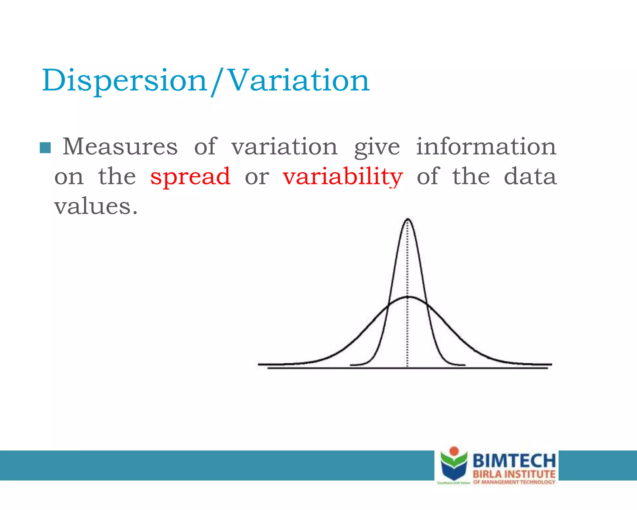
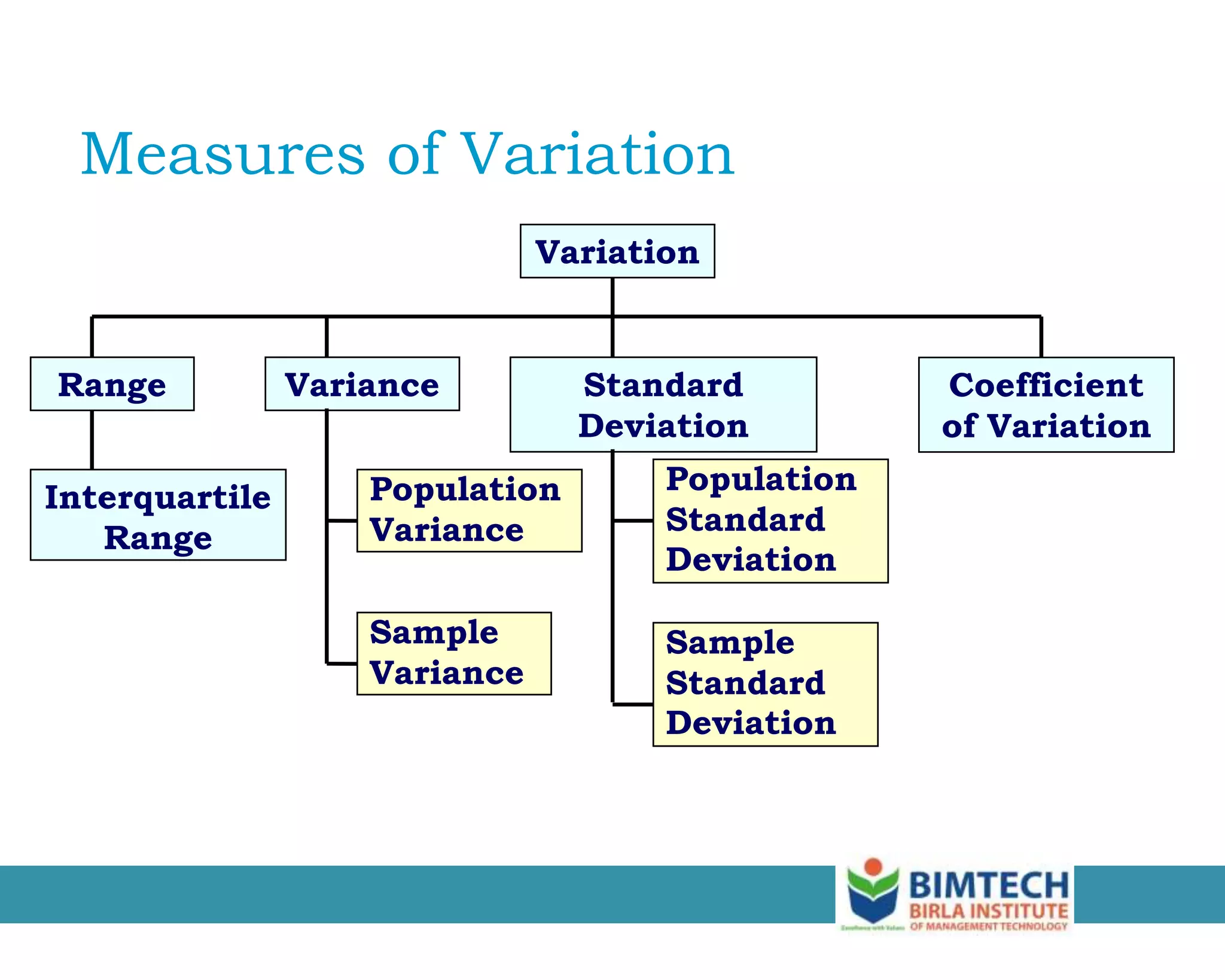
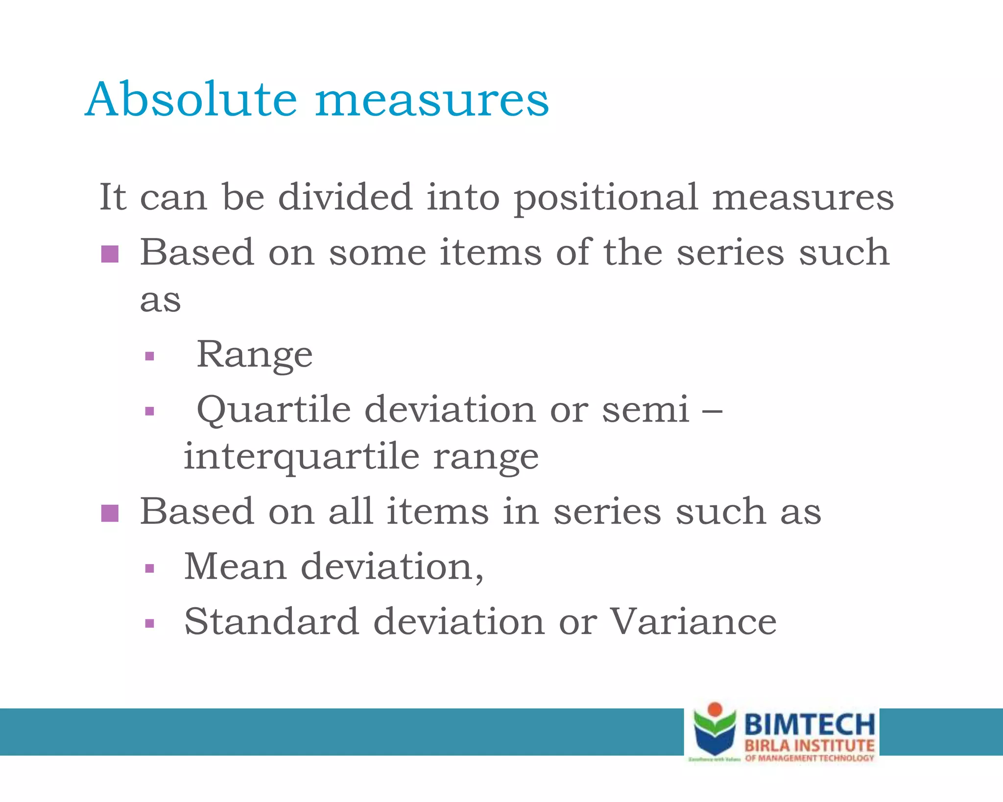
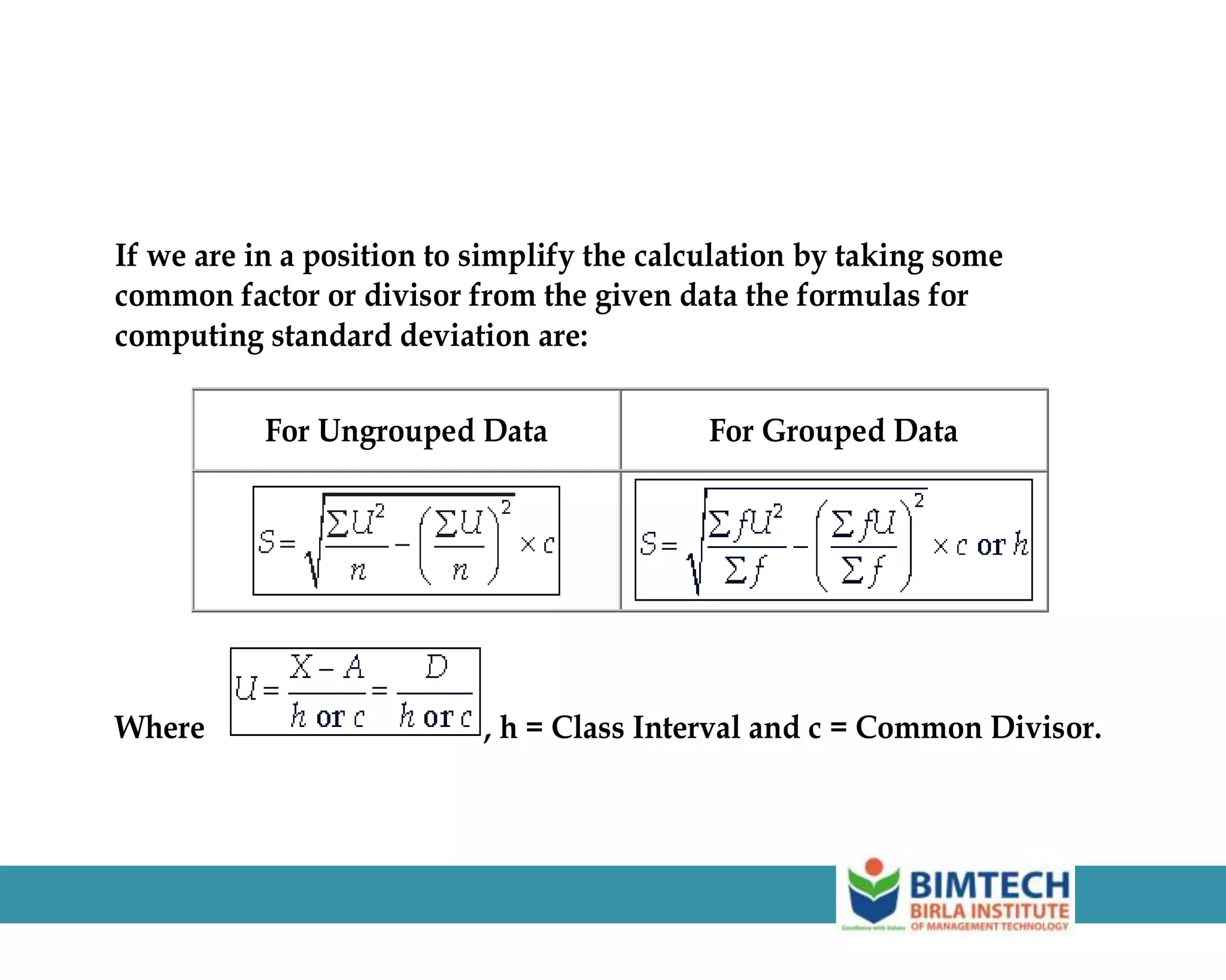
MEASURES OF DISPERSION
Dispersion/Variation
 Measures of variation give information
on the spread or variability of the data
values.
Measures of Variation
Variation
Variance Standard
Deviation
Coefficient
of Variation
Population
Variance
Sample
Variance
Population
Standard
Deviation
Sample
Standard
Deviation
Range
Interquartile
Range
Measure of Dispersion
Measure of Dispersion indicate the spread
of scores
It is necessary to know the amount of
variation and the degree of variation
 absolute measures are used to know the
amount of variation
 relative measures are used to know the
degree of variation
Absolute measures
It can be divided into positional measures
 Based on some items of the series such
as
 Range
 Quartile deviation or semi –
interquartile range
 Based on all items in series such as
 Mean deviation,
 Standard deviation or Variance
Relative measures
It is measuring or estimating things proportionally
to one another. It is used for the comparison
between two or more series with varying size or
number of items, varying central values or units
of calculation.
 Based on some items of the series such as
 Coefficient of Range
 Coefficient of Quartile deviation or semi –
interquartile range
 Based on all items in series such as
 Coefficient of Mean deviation,
 Coefficient of Standard deviation or Variance
Range
 Difference between the largest and the
smallest observations.
Range = xmaximum – xminimum
Example:
0 1 2 3 4 5 6 7 8 9 10 11 12 13 14
Range = 14 - 1 = 13
Coefficient of range /Relative range
Absolute range
= ——————————————
Sum of the two extremes
= xmaximum _ xminimum
xmaximum + xminimum
Example
 SALES FIGURE
 RANGE = H-L = 92-80 = 12
 COEFFICIENT OF RANGE = H-L / H+L
= 92 -80 / 92+80 = 12/172
= 0.069
MONTHLY
SALES
1 2 3 4 5 6
Rs (000) 80 82 82 84 84 86
MONTHLY
SALES
7 8 9 10 11 12
Rs (000) 86 88 88 90 90 92
Disadvantages of the Range
• Ignores the way in which data are distributed
7 8 9 10 11 12
Range = 12 - 7 = 5
7 8 9 10 11 12
Range = 12 - 7 = 5
Sensitive to outliers
Range = 5 - 1 = 4
Range = 120 - 1 = 119
1,1,1,1,1,1,1,1,1,1,1,2,2,2,2,2,2,2,2,3,3,3,3,4,5
1,1,1,1,1,1,1,1,1,1,1,2,2,2,2,2,2,2,2,3,3,3,3,4,120
Mean Deviation
 Mean Deviation can be calculated from
any value of Central Tendency, viz. Mean,
Median, Mode
 Mean Deviation about Mean =
Coefficient of Mean Deviation
Coefficient of Mean Deviation (about mean)
= Mean Deviation
Mean
Coefficient of Mean Deviation (about median)
= Mean Deviation
Median
MEAN DEVIATION FOR GROUPED
DATA FORMULA
Example
Calculate the mean deviation from
(1) arithmetic mean
(2) median
(3) mode
with respect of the marks obtained by nine
students gives below and show that the
mean deviation from median is
minimum. Marks (out of 25): 7, 4, 10, 9,
15, 12, 7, 9, 7
Solution
After arranging the observations in ascending order,
we get Marks:
4, 7, 7, 7, 9, 9, 10, 12, 15
Mode = 7 (Since 7 is repeated maximum number of times)
Marks X
4 4.89 5 3
7 1.89 2 0
7 1.89 2 0
7 1.89 2 0
9 0.11 0 2
9 0.11 0 2
10 1.11 1 3
12 3.11 3 5
15 6.11 6 8
Total 21.11 21 23
From the above calculations, it is clear that the mean deviation from the
median has the least value.
FIND AVERAGE DEVIATION
OF GIVEN DATA
DIVIDE
ND
YIELD
NO OF
COMPA
NIES (f)
MID
POINT
( m)
fm X-µ I X - µ I f . I X - µ I
0-3 2
3-6 7
6-9 10
9-12 12
12-15 9
15-18 6
18-21 4
Variance
 Average of squared deviations of values
from the mean
N
μ)
(x
σ
N
1
i
2
i
2




Standard Deviation
 Most commonly used measure of variation
 Shows variation about the mean
 Has the same units as the original data
Actual Mean Method
For UngroupedData For GroupedData
Assumed Mean Method (short
cut method)
For UngroupedData For GroupedData
Where andA is any assumedmeanother thanzero. This
methodis also knownas short-cut method.
If we are in a position to simplify the calculation by taking some
common factor or divisor from the given data the formulas for
computing standard deviation are:
For Ungrouped Data For Grouped Data
Where , h = Class Interval and c = Common Divisor.
Calculation Example: Sample
Standard Deviation
Sample
Data (Xi) : 10 12 14 15 17 18 18 24
n = 8 Mean = x = 16
4.2426
7
126
1
8
16)
(24
16)
(14
16)
(12
16)
(10
1
n
)
x
(24
)
x
(14
)
x
(12
)
x
(10
s
2
2
2
2
2
2
2
2
























Mean = 15.5
s = 3.338
11 12 13 14 15 16 17 18 19 20 21
Data B
Data A
Mean = 15.5
s = .9258
Mean = 15.5
s = 4.57
Data C
11 12 13 14 15 16 17 18 19 20 21
11 12 13 14 15 16 17 18 19 20 21
Comparing Standard Deviations
 Calculate standard deviation from the
following distribution of marks
Marks No. of Students
1-3 40
3-5 30
5-7 20
7-9 10
Solution:
Method-I: Actual Mean Method
Marks f X fX
Total
Marks
Method-II: Taking assumed mean as 2
Marks f X D=(X-2) fD fD2
Total
Marks
Method-III: By taking 2 as the common divisor
Marks f X u = (X-2)/2 fu fu2
Total
Marks
Coefficient of Variation
 Measures relative variation
 Always in percentage (%)
 Shows variation relative to mean
 Is used to compare two or more sets of
data measured in different units
100%
x
s
CV 









A distribution is x = 140 and σ = 28.28 and the
other is x = 150 and σ = 25. Which of the two
has a greater dispersion?
The first distribution has a greater dispersion.
Comparing Coefficient of Variation
 Stock A:
◦ Average price last year = $50
◦ Standard deviation = $5
Stock B:
Average price last year = $100
Standard deviation = $5
10%
100%
$50
$5
100%
x
s
CVA 












5%
100%
$100
$5
100%
x
s
CVB 












Both stocks
have the same
standard
deviation, but
stock B is less
variable
relative to its
price
SKEWNESS and Kurtosis
Skewness
Skewness refers to lack of symmetry or departure from
symmetry.
If the value of mean is greater than mode then distribution is
positively skewed.
If the value of mean is less than mode then distribution is
negatively skewed
Measure of Skewness
Skweness =
Where
S = standard deviation
N = number of data points
Mean Y = mean of the data
Kurtosis
Kurtosis means : “bulginess”
Kurtosis is the degree of peakedness of a distribution
usually taken relative to a normal distribution.
 A distribution having a relatively high peak is called
‘leptokurtic’.
 A distribution which plat topped is called
‘platykurtic’.
 A normal distribution which is neither very peaked
nor very flat-topped is also called ‘mesokurtic’.
 Kurtosis is measured by a quantity denoted by β2
where:
β2 =
Where
S = standard deviation
N = number of data points
Mean Y = mean of the data
 If β2 = 3, it is mesokurtic or normal,
 If β2 > 3, it is leptokurtic, and
 If β2 < 3, it platykurtic.
Measures of Kurtosis
Difference between Variation
and Skewness
 Variation tells about the amount of the variation or
dispersion in the data. Skewness tells us about the
direction of variation.
 In business and economic series, measures of variation
have greater practical applications than measures of
skewness.

Measures of Dispersion .pptx

  • 1.
  • 2.
    Dispersion/Variation  Measures ofvariation give information on the spread or variability of the data values.
  • 3.
    Measures of Variation Variation VarianceStandard Deviation Coefficient of Variation Population Variance Sample Variance Population Standard Deviation Sample Standard Deviation Range Interquartile Range
  • 4.
    Measure of Dispersion Measureof Dispersion indicate the spread of scores It is necessary to know the amount of variation and the degree of variation  absolute measures are used to know the amount of variation  relative measures are used to know the degree of variation
  • 5.
    Absolute measures It canbe divided into positional measures  Based on some items of the series such as  Range  Quartile deviation or semi – interquartile range  Based on all items in series such as  Mean deviation,  Standard deviation or Variance
  • 6.
    Relative measures It ismeasuring or estimating things proportionally to one another. It is used for the comparison between two or more series with varying size or number of items, varying central values or units of calculation.  Based on some items of the series such as  Coefficient of Range  Coefficient of Quartile deviation or semi – interquartile range  Based on all items in series such as  Coefficient of Mean deviation,  Coefficient of Standard deviation or Variance
  • 7.
    Range  Difference betweenthe largest and the smallest observations. Range = xmaximum – xminimum Example: 0 1 2 3 4 5 6 7 8 9 10 11 12 13 14 Range = 14 - 1 = 13
  • 8.
    Coefficient of range/Relative range Absolute range = —————————————— Sum of the two extremes = xmaximum _ xminimum xmaximum + xminimum
  • 9.
    Example  SALES FIGURE RANGE = H-L = 92-80 = 12  COEFFICIENT OF RANGE = H-L / H+L = 92 -80 / 92+80 = 12/172 = 0.069 MONTHLY SALES 1 2 3 4 5 6 Rs (000) 80 82 82 84 84 86 MONTHLY SALES 7 8 9 10 11 12 Rs (000) 86 88 88 90 90 92
  • 10.
    Disadvantages of theRange • Ignores the way in which data are distributed 7 8 9 10 11 12 Range = 12 - 7 = 5 7 8 9 10 11 12 Range = 12 - 7 = 5 Sensitive to outliers Range = 5 - 1 = 4 Range = 120 - 1 = 119 1,1,1,1,1,1,1,1,1,1,1,2,2,2,2,2,2,2,2,3,3,3,3,4,5 1,1,1,1,1,1,1,1,1,1,1,2,2,2,2,2,2,2,2,3,3,3,3,4,120
  • 11.
    Mean Deviation  MeanDeviation can be calculated from any value of Central Tendency, viz. Mean, Median, Mode  Mean Deviation about Mean =
  • 12.
    Coefficient of MeanDeviation Coefficient of Mean Deviation (about mean) = Mean Deviation Mean Coefficient of Mean Deviation (about median) = Mean Deviation Median
  • 13.
    MEAN DEVIATION FORGROUPED DATA FORMULA
  • 14.
    Example Calculate the meandeviation from (1) arithmetic mean (2) median (3) mode with respect of the marks obtained by nine students gives below and show that the mean deviation from median is minimum. Marks (out of 25): 7, 4, 10, 9, 15, 12, 7, 9, 7
  • 15.
    Solution After arranging theobservations in ascending order, we get Marks: 4, 7, 7, 7, 9, 9, 10, 12, 15 Mode = 7 (Since 7 is repeated maximum number of times)
  • 16.
    Marks X 4 4.895 3 7 1.89 2 0 7 1.89 2 0 7 1.89 2 0 9 0.11 0 2 9 0.11 0 2 10 1.11 1 3 12 3.11 3 5 15 6.11 6 8 Total 21.11 21 23
  • 17.
    From the abovecalculations, it is clear that the mean deviation from the median has the least value.
  • 18.
    FIND AVERAGE DEVIATION OFGIVEN DATA DIVIDE ND YIELD NO OF COMPA NIES (f) MID POINT ( m) fm X-µ I X - µ I f . I X - µ I 0-3 2 3-6 7 6-9 10 9-12 12 12-15 9 15-18 6 18-21 4
  • 19.
    Variance  Average ofsquared deviations of values from the mean N μ) (x σ N 1 i 2 i 2    
  • 20.
    Standard Deviation  Mostcommonly used measure of variation  Shows variation about the mean  Has the same units as the original data
  • 21.
    Actual Mean Method ForUngroupedData For GroupedData
  • 22.
    Assumed Mean Method(short cut method) For UngroupedData For GroupedData Where andA is any assumedmeanother thanzero. This methodis also knownas short-cut method.
  • 23.
    If we arein a position to simplify the calculation by taking some common factor or divisor from the given data the formulas for computing standard deviation are: For Ungrouped Data For Grouped Data Where , h = Class Interval and c = Common Divisor.
  • 24.
    Calculation Example: Sample StandardDeviation Sample Data (Xi) : 10 12 14 15 17 18 18 24 n = 8 Mean = x = 16 4.2426 7 126 1 8 16) (24 16) (14 16) (12 16) (10 1 n ) x (24 ) x (14 ) x (12 ) x (10 s 2 2 2 2 2 2 2 2                        
  • 25.
    Mean = 15.5 s= 3.338 11 12 13 14 15 16 17 18 19 20 21 Data B Data A Mean = 15.5 s = .9258 Mean = 15.5 s = 4.57 Data C 11 12 13 14 15 16 17 18 19 20 21 11 12 13 14 15 16 17 18 19 20 21 Comparing Standard Deviations
  • 26.
     Calculate standarddeviation from the following distribution of marks Marks No. of Students 1-3 40 3-5 30 5-7 20 7-9 10
  • 27.
    Solution: Method-I: Actual MeanMethod Marks f X fX Total Marks
  • 28.
    Method-II: Taking assumedmean as 2 Marks f X D=(X-2) fD fD2 Total Marks
  • 29.
    Method-III: By taking2 as the common divisor Marks f X u = (X-2)/2 fu fu2 Total Marks
  • 30.
    Coefficient of Variation Measures relative variation  Always in percentage (%)  Shows variation relative to mean  Is used to compare two or more sets of data measured in different units 100% x s CV          
  • 31.
    A distribution isx = 140 and σ = 28.28 and the other is x = 150 and σ = 25. Which of the two has a greater dispersion? The first distribution has a greater dispersion.
  • 32.
    Comparing Coefficient ofVariation  Stock A: ◦ Average price last year = $50 ◦ Standard deviation = $5 Stock B: Average price last year = $100 Standard deviation = $5 10% 100% $50 $5 100% x s CVA              5% 100% $100 $5 100% x s CVB              Both stocks have the same standard deviation, but stock B is less variable relative to its price
  • 33.
  • 34.
    Skewness Skewness refers tolack of symmetry or departure from symmetry. If the value of mean is greater than mode then distribution is positively skewed. If the value of mean is less than mode then distribution is negatively skewed
  • 35.
    Measure of Skewness Skweness= Where S = standard deviation N = number of data points Mean Y = mean of the data
  • 36.
    Kurtosis Kurtosis means :“bulginess” Kurtosis is the degree of peakedness of a distribution usually taken relative to a normal distribution.  A distribution having a relatively high peak is called ‘leptokurtic’.  A distribution which plat topped is called ‘platykurtic’.  A normal distribution which is neither very peaked nor very flat-topped is also called ‘mesokurtic’.
  • 37.
     Kurtosis ismeasured by a quantity denoted by β2 where: β2 = Where S = standard deviation N = number of data points Mean Y = mean of the data  If β2 = 3, it is mesokurtic or normal,  If β2 > 3, it is leptokurtic, and  If β2 < 3, it platykurtic. Measures of Kurtosis
  • 39.
    Difference between Variation andSkewness  Variation tells about the amount of the variation or dispersion in the data. Skewness tells us about the direction of variation.  In business and economic series, measures of variation have greater practical applications than measures of skewness.

Editor's Notes