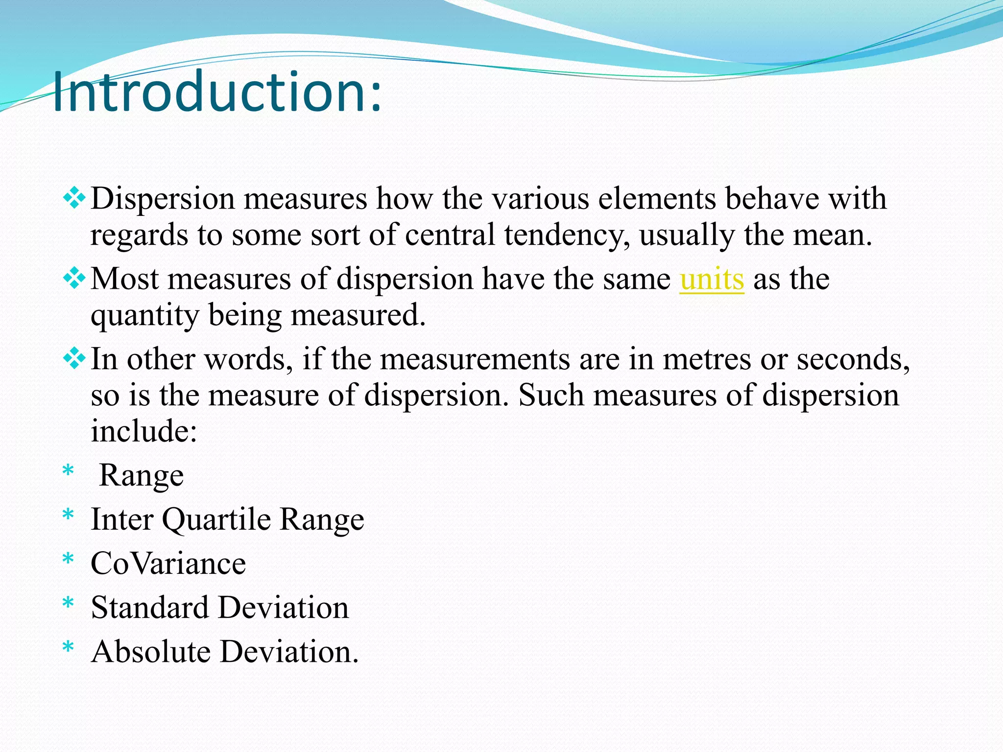
This document discusses various measures of dispersion, which refer to how spread out or varied a set of data is from a central value. It describes standard deviation, which quantifies how far data points deviate from the mean on average. A lower standard deviation indicates less volatility or risk. The coefficient of variation allows comparison of volatility relative to expected returns. The range is the maximum minus minimum value but can be skewed by outliers, while the interquartile range ignores the highest and lowest quartiles to better represent the middle data.

2. Introduction:
Dispersion measures how the various elements behave with
regards to some sort of central tendency, usually the mean.
Most measures of dispersion have the same units as the
quantity being measured.
In other words, if the measurements are in metres or seconds,
so is the measure of dispersion. Such measures of dispersion
include:
* Range
* Inter Quartile Range
* CoVariance
* Standard Deviation
* Absolute Deviation.

3. Variance and Standard Deviation:
Standard Deviation:
* A measure of the dispersion of a set of data from its mean. The
more spread apart the data, the higher the deviation. Standard
deviation is calculated as the square root of variance.
* Standard deviation is a statistical measurement that sheds light
on historical volatility.
* For example, a volatile stock will have a high standard
deviation while the deviation of a stable blue chip stock will be
lower. A large dispersion tells us how much the return on the
fund is deviating from the expected normal returns.

4. Coefficient of Variance:
* The coefficient of variation represents the ratio of the standard
deviation to the mean, and it is a useful statistic for comparing
the degree of variation from one data series to another, even if
the means are drastically different from each other.
* In the investing world, the coefficient of variation allows you
to determine how much volatility (risk) you are assuming in
comparison to the amount of return you can expect from your
investment. In simple language, the lower the ratio of standard
deviation to mean return, the better your risk-return tradeoff.

5. Range and Inter Quartile Range
Range:
 Range is defined simply as the difference between the
maximum and minimum observations.
 Range is quite a useful indication of how spread out the
data is, but it has some serious limitations. This is because
sometimes data can have outliers that are widely off the
other data points. In these cases, the range might not give
a true indication of the spread of data.

6. Inter Quartile Range:
•The interquartile range (IQR) is a measure of variability, based on dividing a data
set into quartiles.
•Quartiles divide a rank-ordered data set into four equal parts. The values that divide
each part are called the first, second, and third quartiles; and they are denoted by Q1,
Q2, and Q3, respectively.
Q1 is the "middle" value in the first half of the rank-ordered data set.
Q2 is the median value in the set.
Q3 is the "middle" value in the second half of the rank-ordered data set.
The interquartile range is equal to Q3 minus Q1.
IQR = Q3 − Q1