Downloaded 185 times


![• Example : In a moderately symmetrical distribution –Example : In a moderately symmetrical distribution –
The mode and median are 75 and 60 respectively.The mode and median are 75 and 60 respectively.
Find Mean.Find Mean.
• Solution : Using the empirical relation betweenSolution : Using the empirical relation between
Mean/Median/Mode, we can writeMean/Median/Mode, we can write
Mean – Mode = 3 (Mean – Median)Mean – Mode = 3 (Mean – Median)
0R0R
2 Mean = 3 Median – Mode2 Mean = 3 Median – Mode
Hence,Hence,
Mean = [3 Median – Mode] / 2 = [3(60) – 75] / 2 = 52.5Mean = [3 Median – Mode] / 2 = [3(60) – 75] / 2 = 52.5](https://image.slidesharecdn.com/measuresofcentraltendency-160707094720/75/Measures-of-central-tendency-68-2048.jpg)


The document discusses various measures of central tendency including the mean, median, and mode. It provides definitions and formulas for calculating the arithmetic mean, weighted arithmetic mean, mean of composite groups, and harmonic mean. The arithmetic mean is calculated by summing all values and dividing by the total number of values. It is impacted by outliers. The harmonic mean gives more weight to smaller values and is used to average rates or speeds. Examples are provided to demonstrate calculating the different types of means.
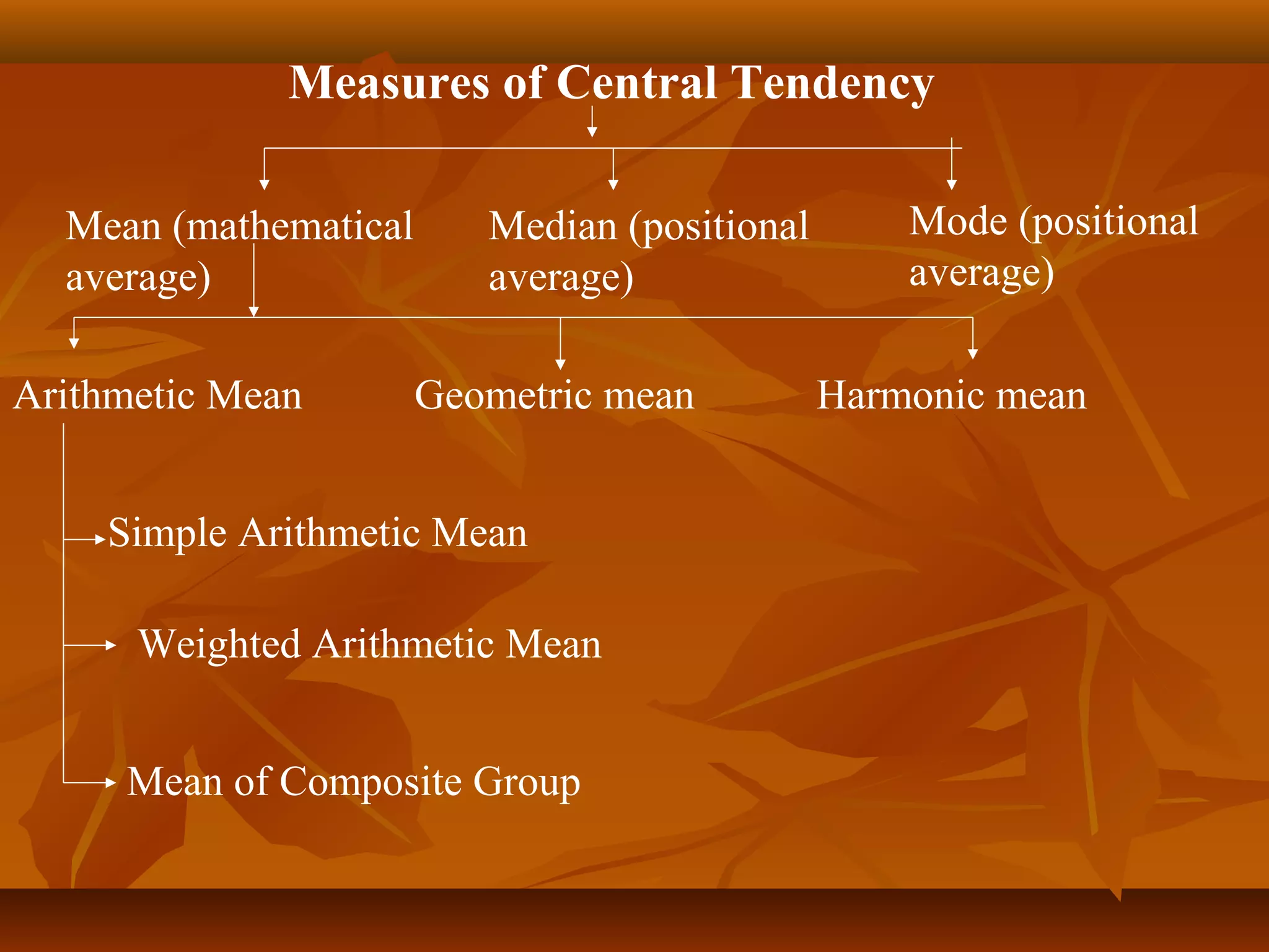
Introduction to the concept of central tendency, defining measures like mean, median, mode.
Types of measures: Mean (arithmetic, geometric, harmonic), Median, and Mode. Definition and basic understanding.
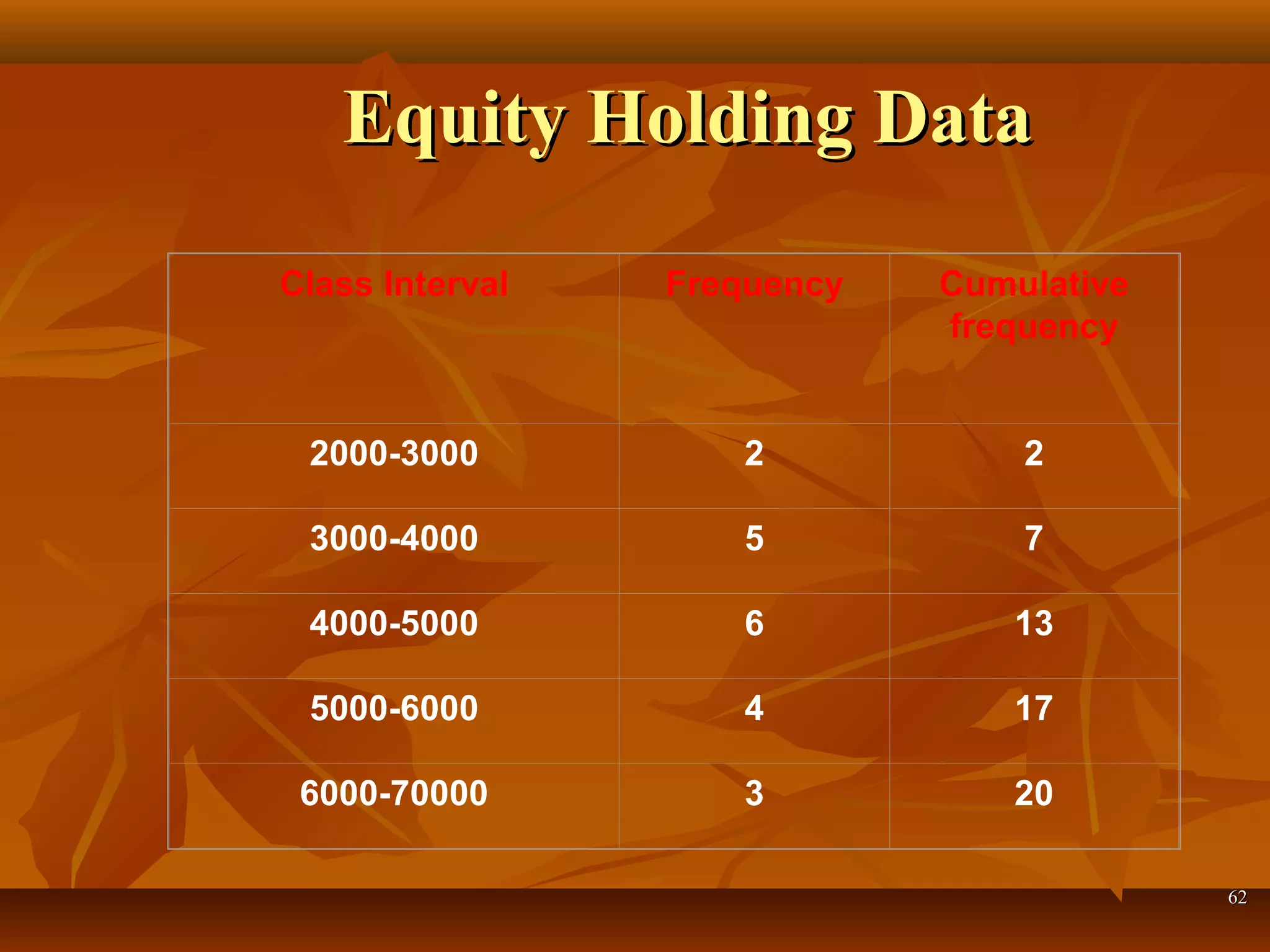
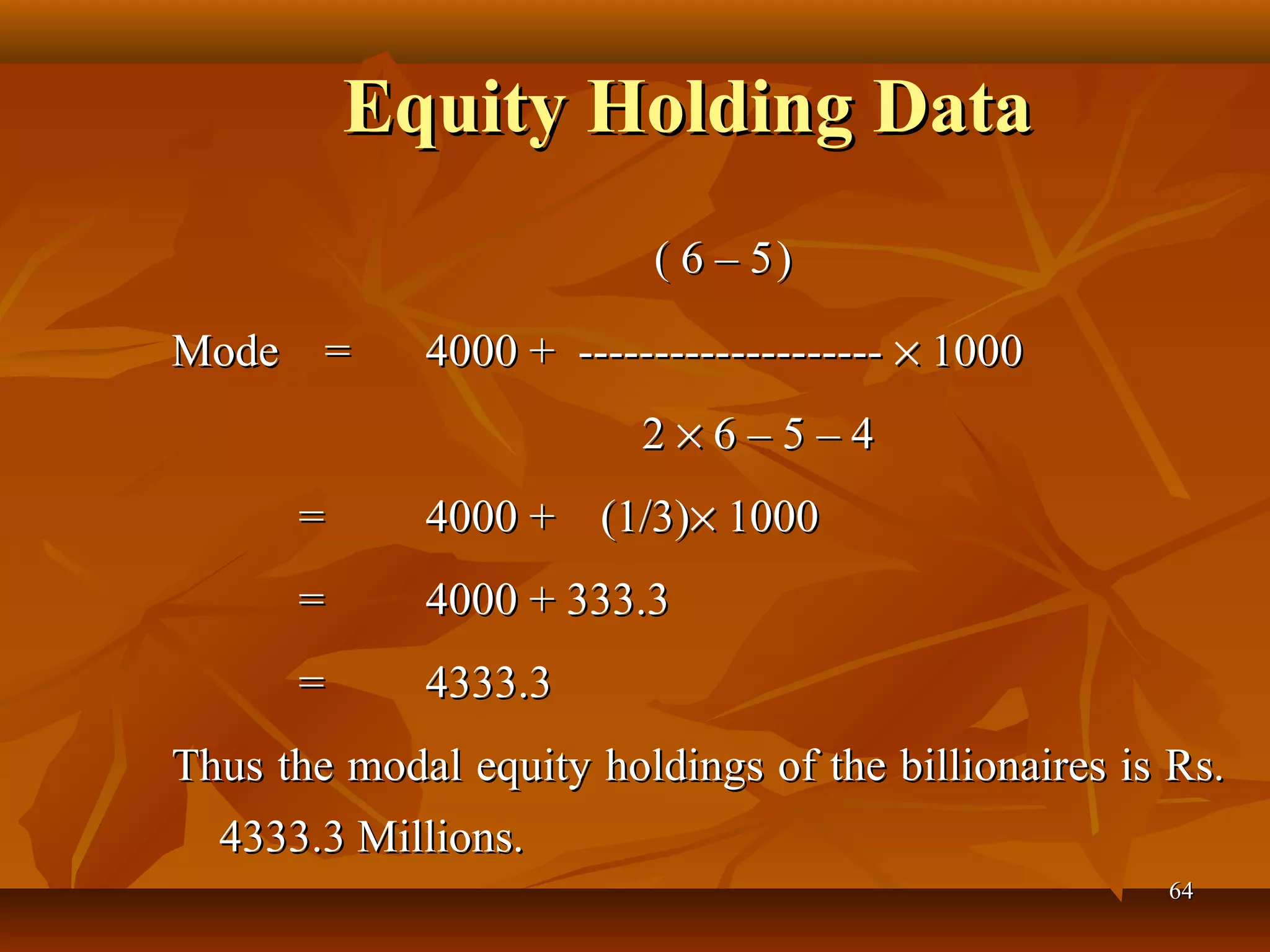
Formula for calculating arithmetic mean using ungrouped data, with a practical example of billionaires' equity.
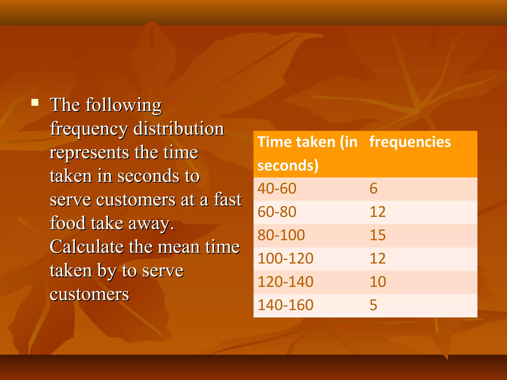
Calculating arithmetic mean for grouped data and understanding mid values, with examples on salary and pressure.
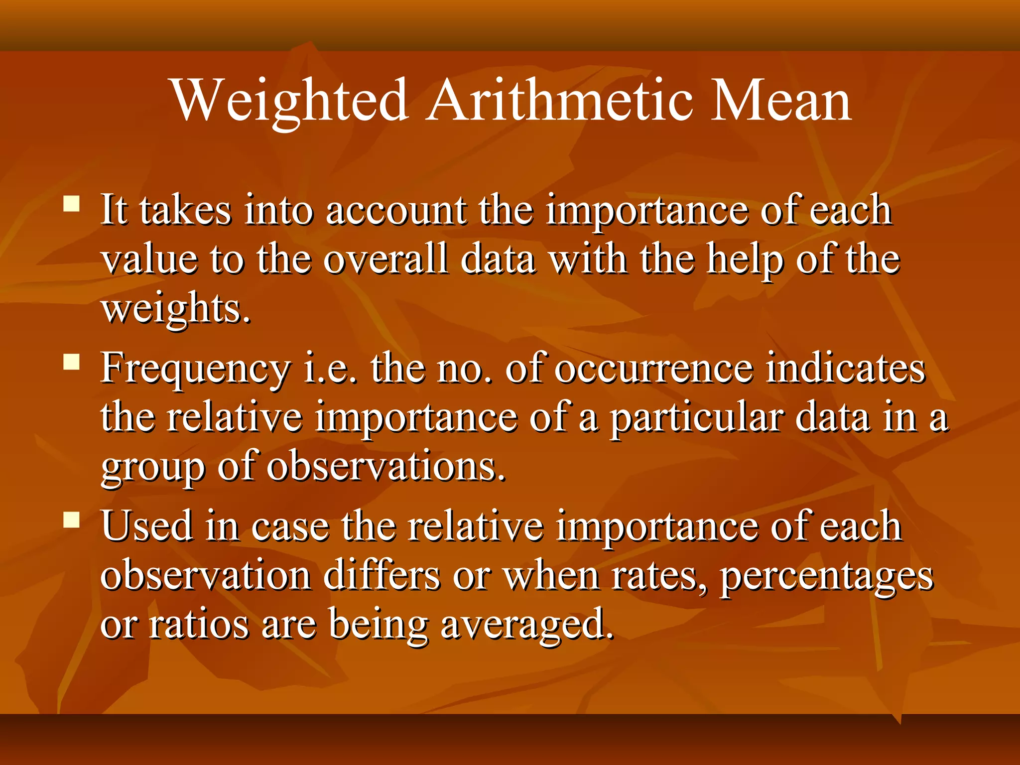
Concept of weighted arithmetic mean, its importance, and an example of student's performance calculation.
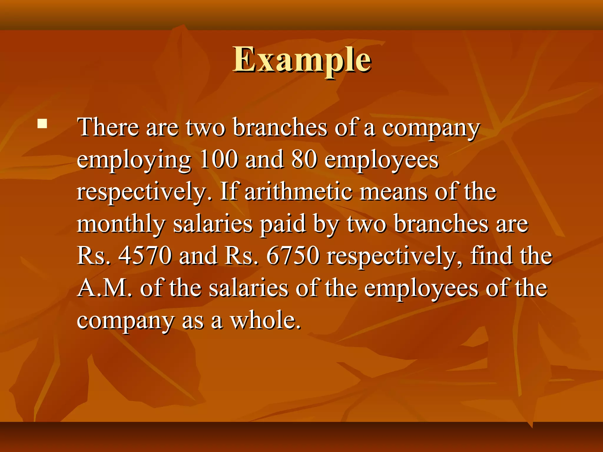
Formula for mean of composite groups and examples of salary calculations in branches of a company.
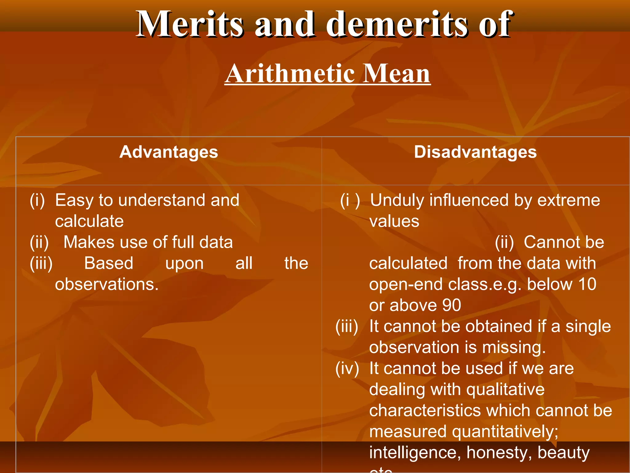
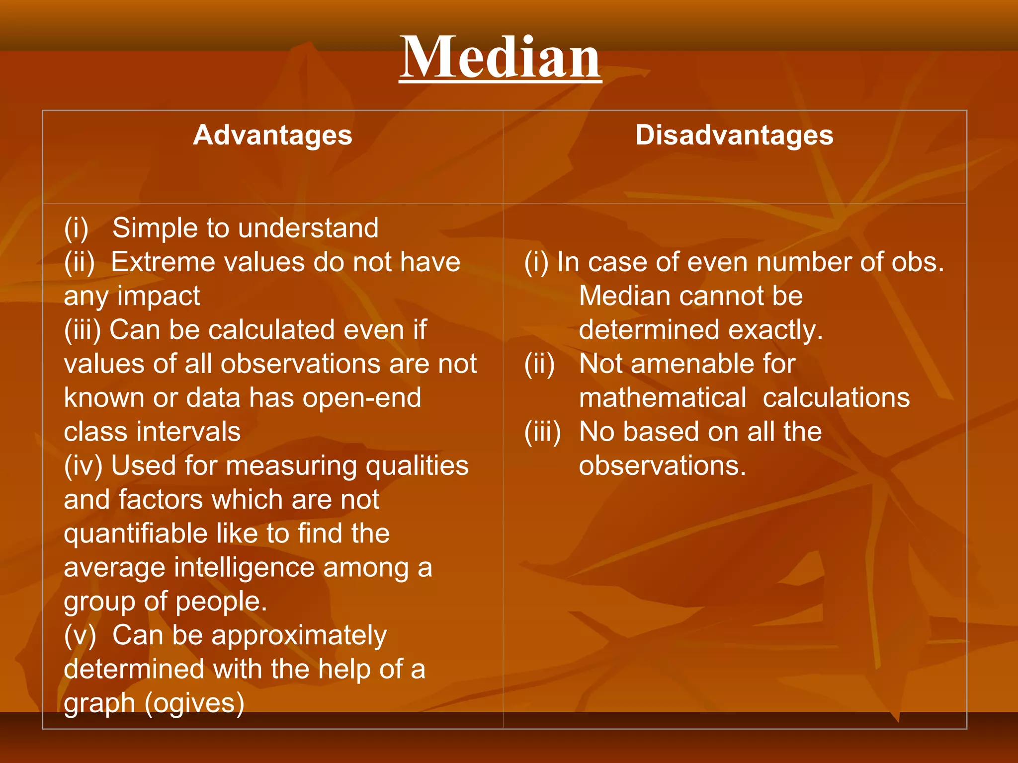
Properties of arithmetic mean, its merits, demerits, and introduction to harmonic mean.
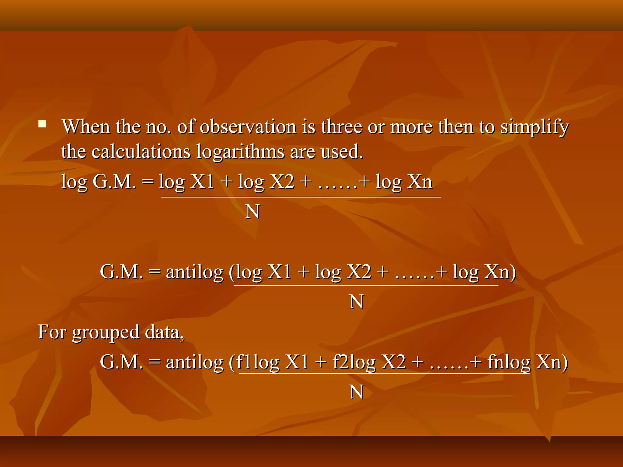
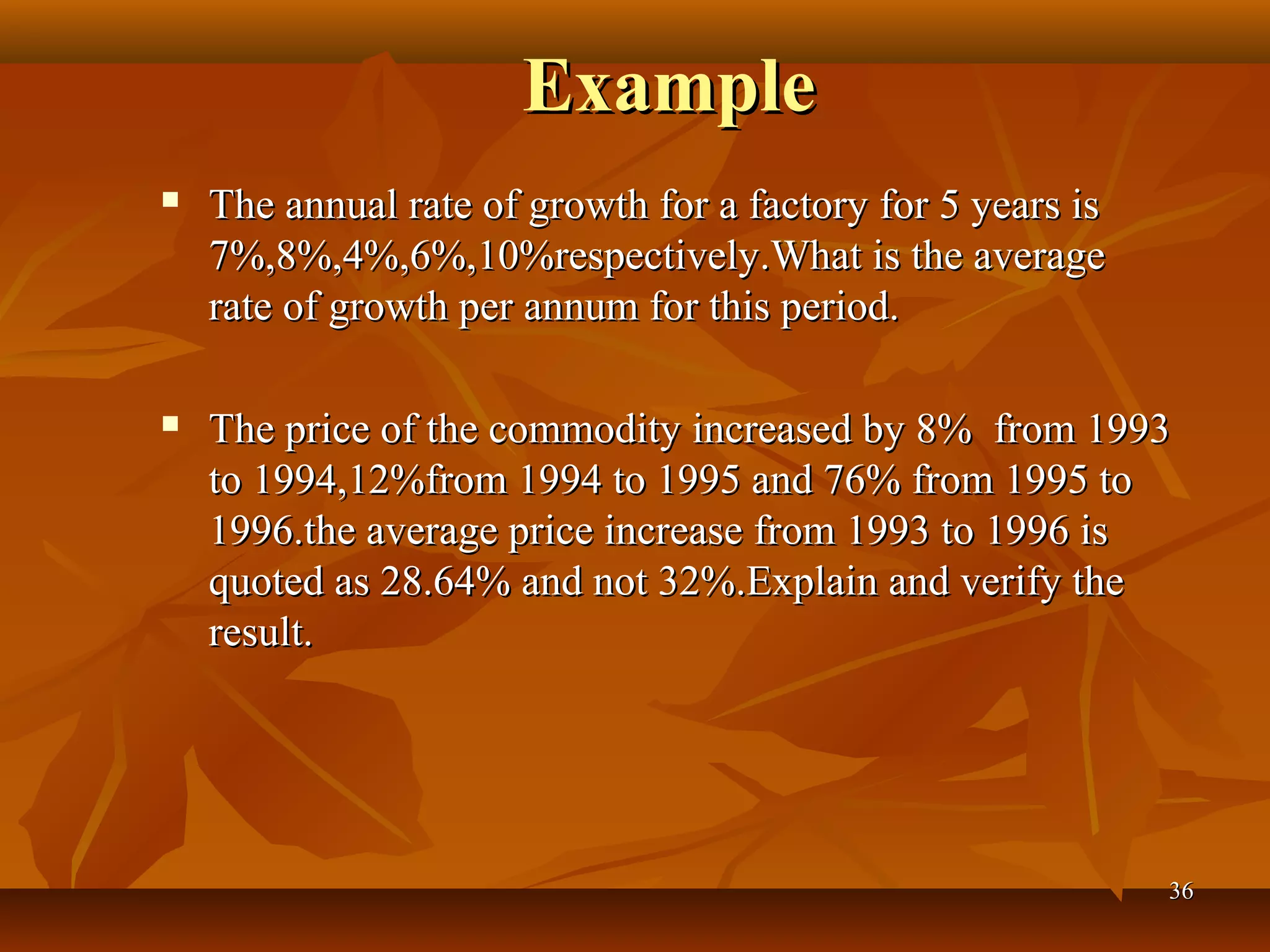
Definition and application of geometric mean in rates of change, especially in finance and growth.
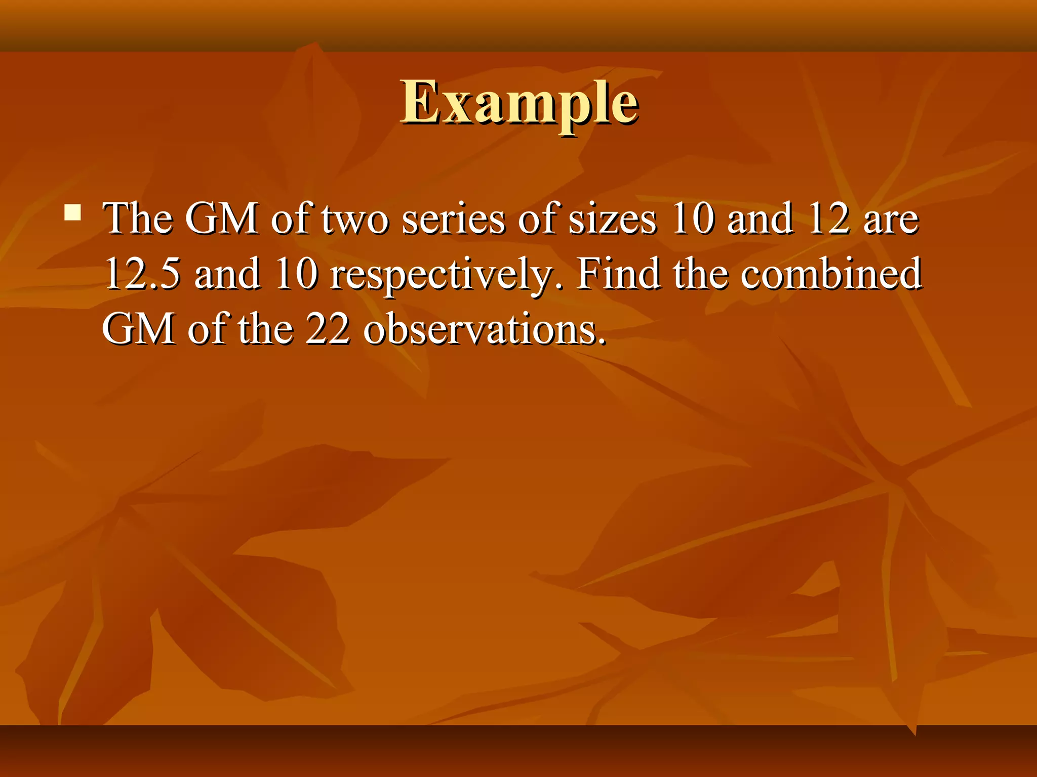
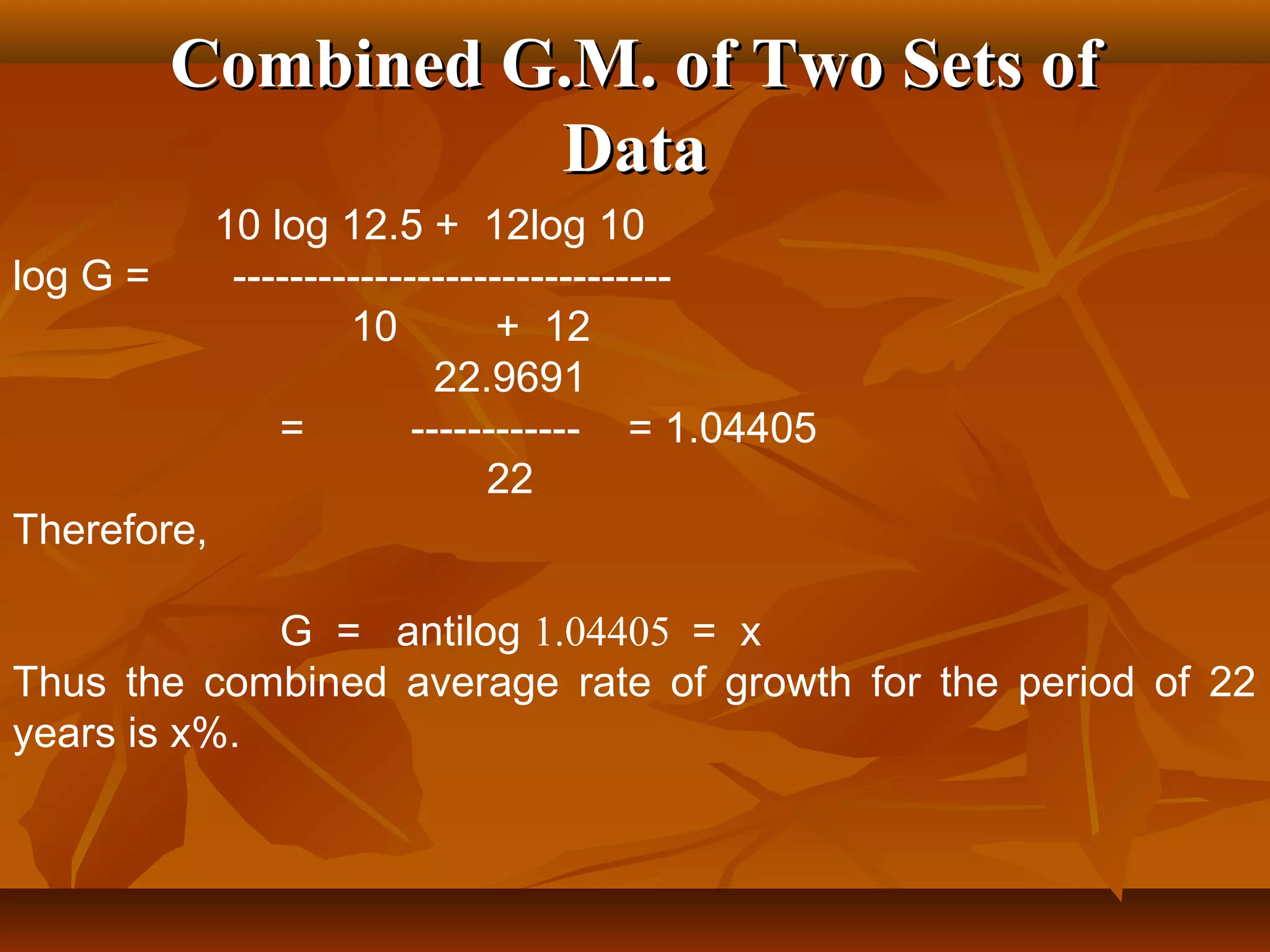
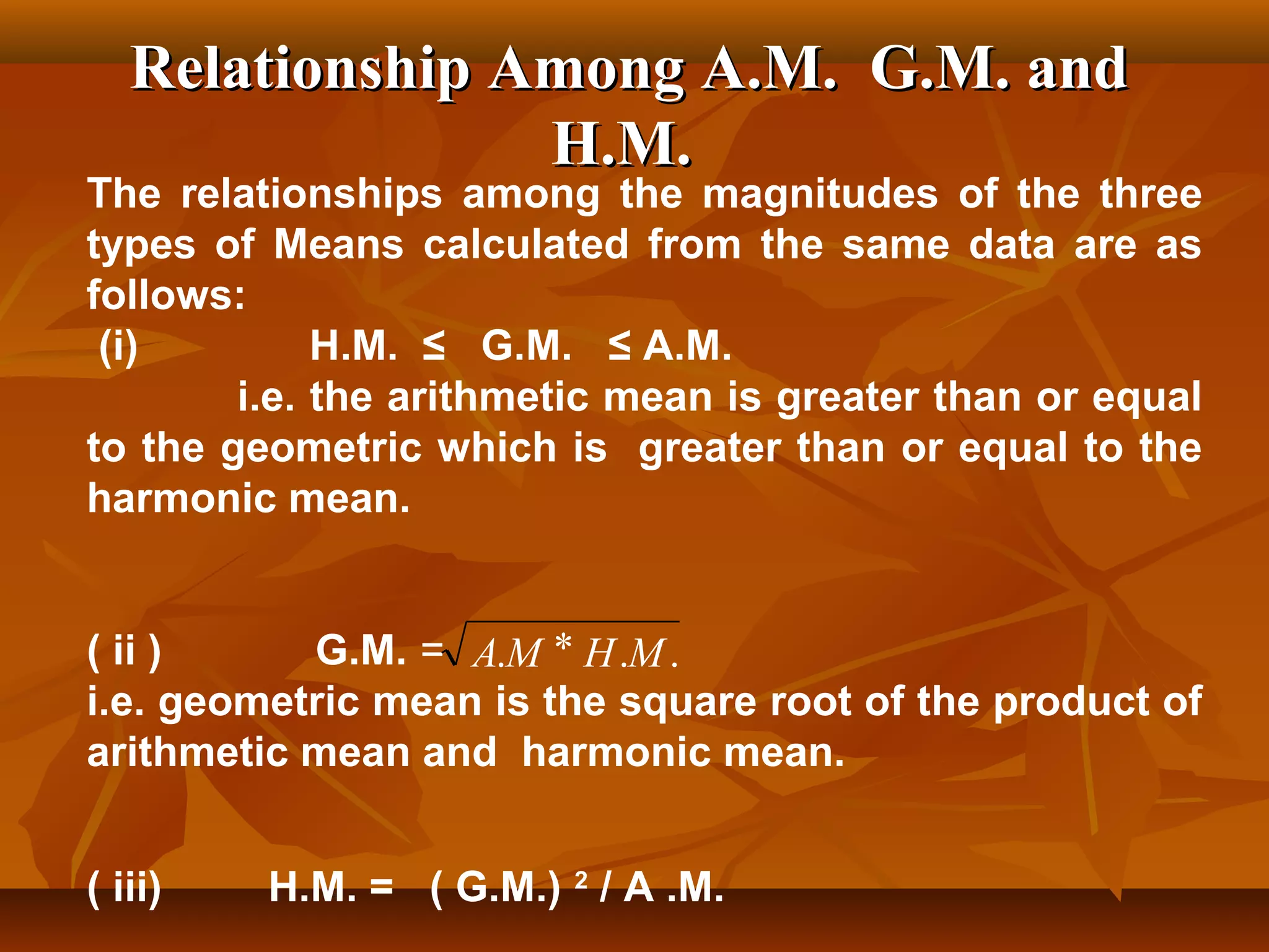
Calculating combined geometric mean for two sets and relationship among A.M., G.M., and H.M.
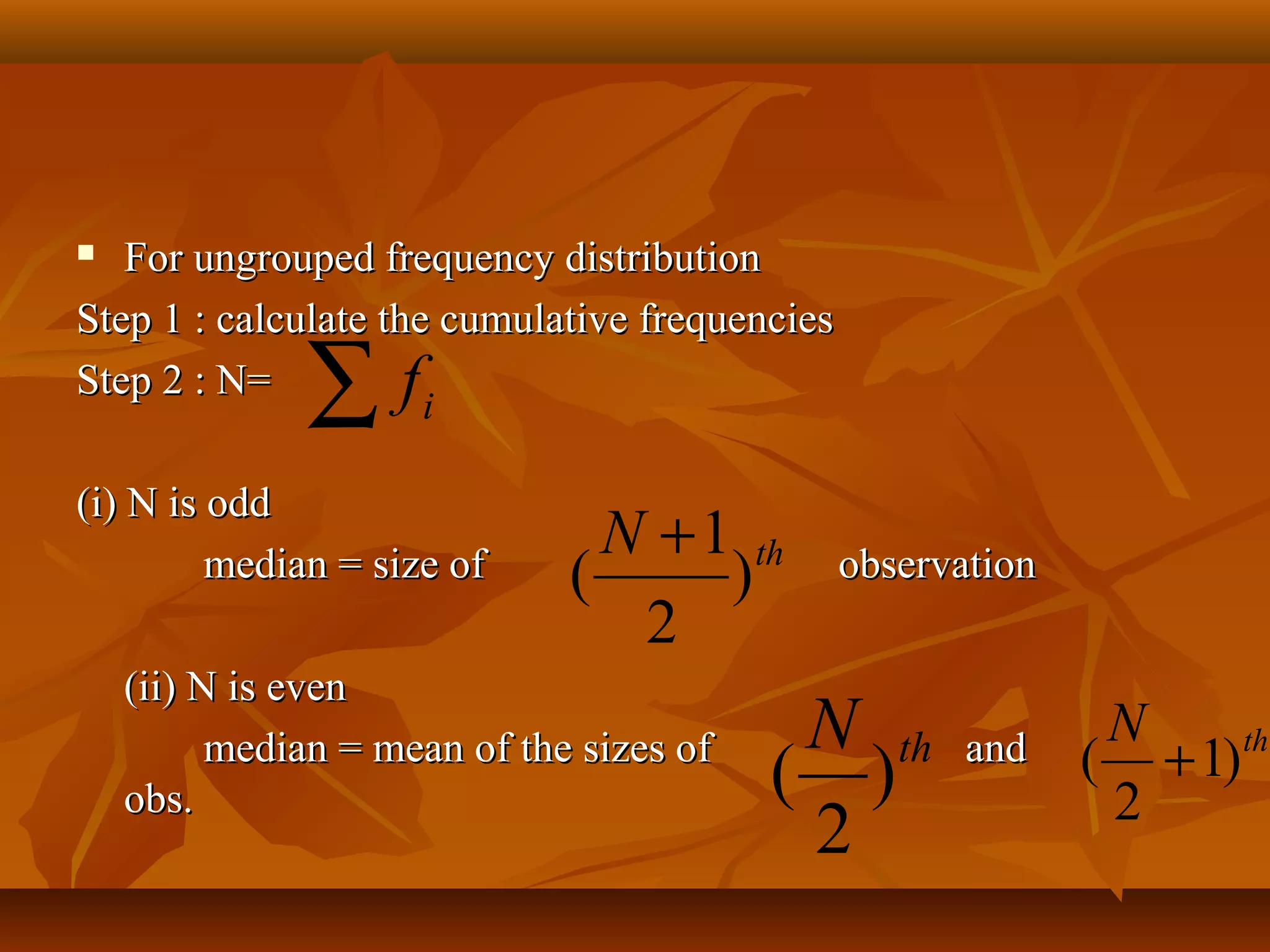
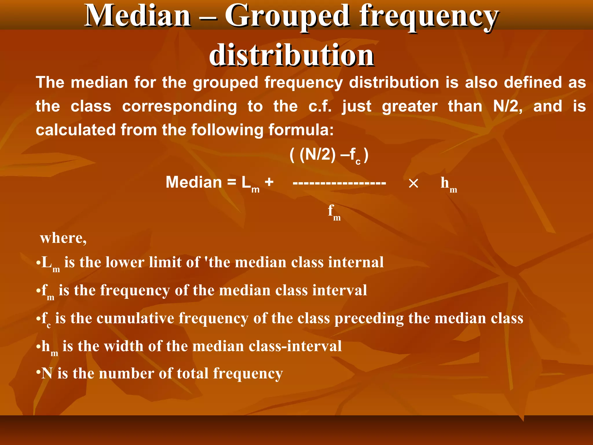
Definition of median, its calculation methods, and its importance in skewed distributions.
Example for calculating median from ungrouped data for observations like company profits.
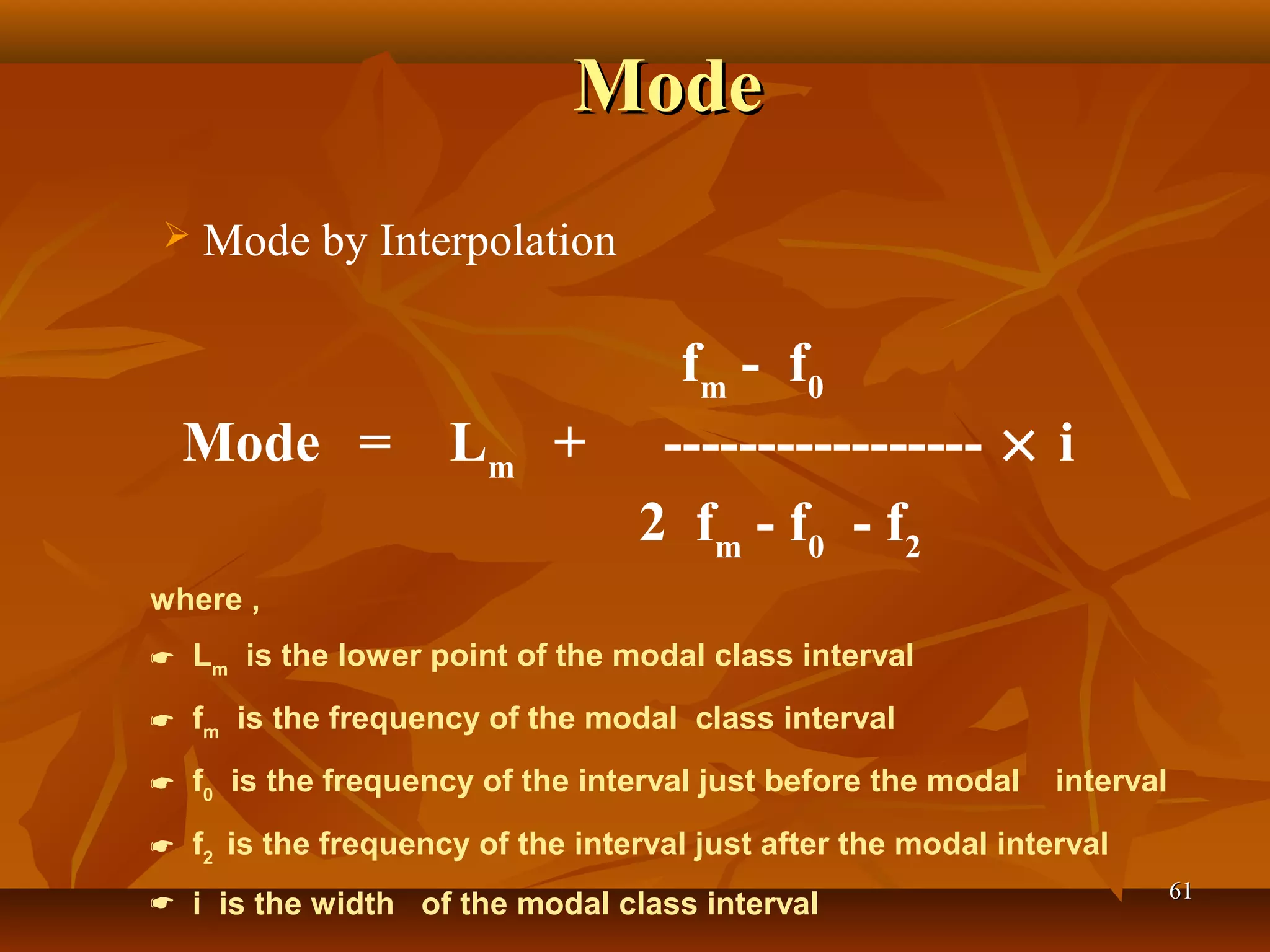
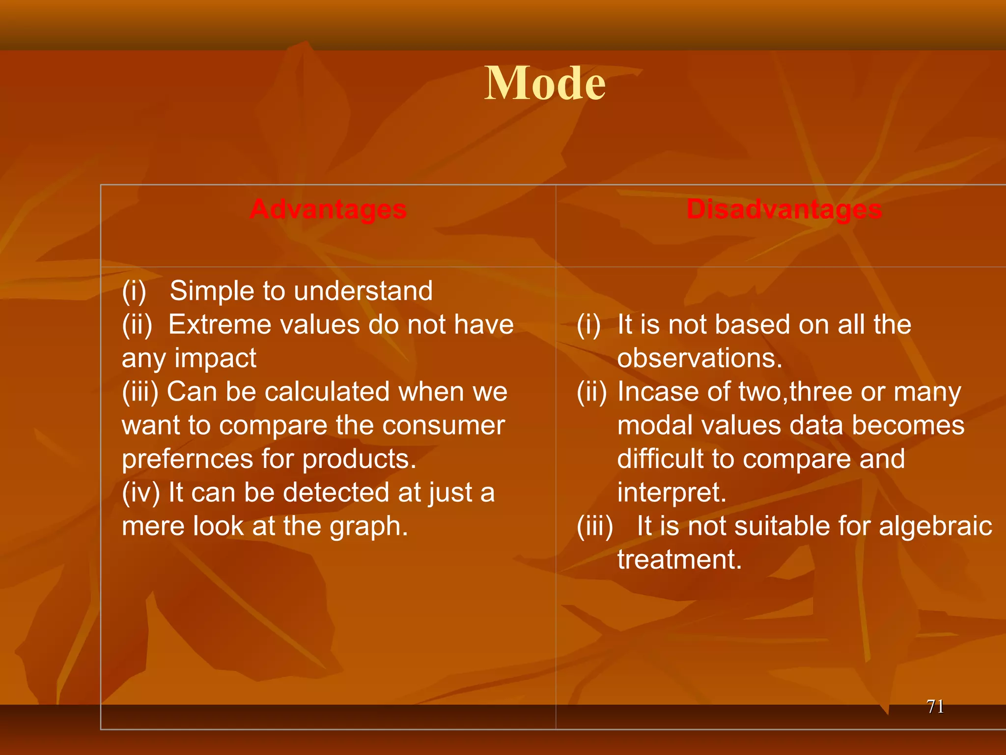
Definition of mode, methods of finding mode, its types, and applications.
Calculating mean, median, mode relationships in distributions and empirical relationship graphically.
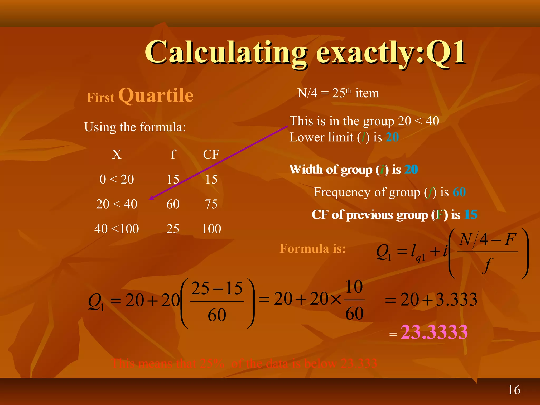
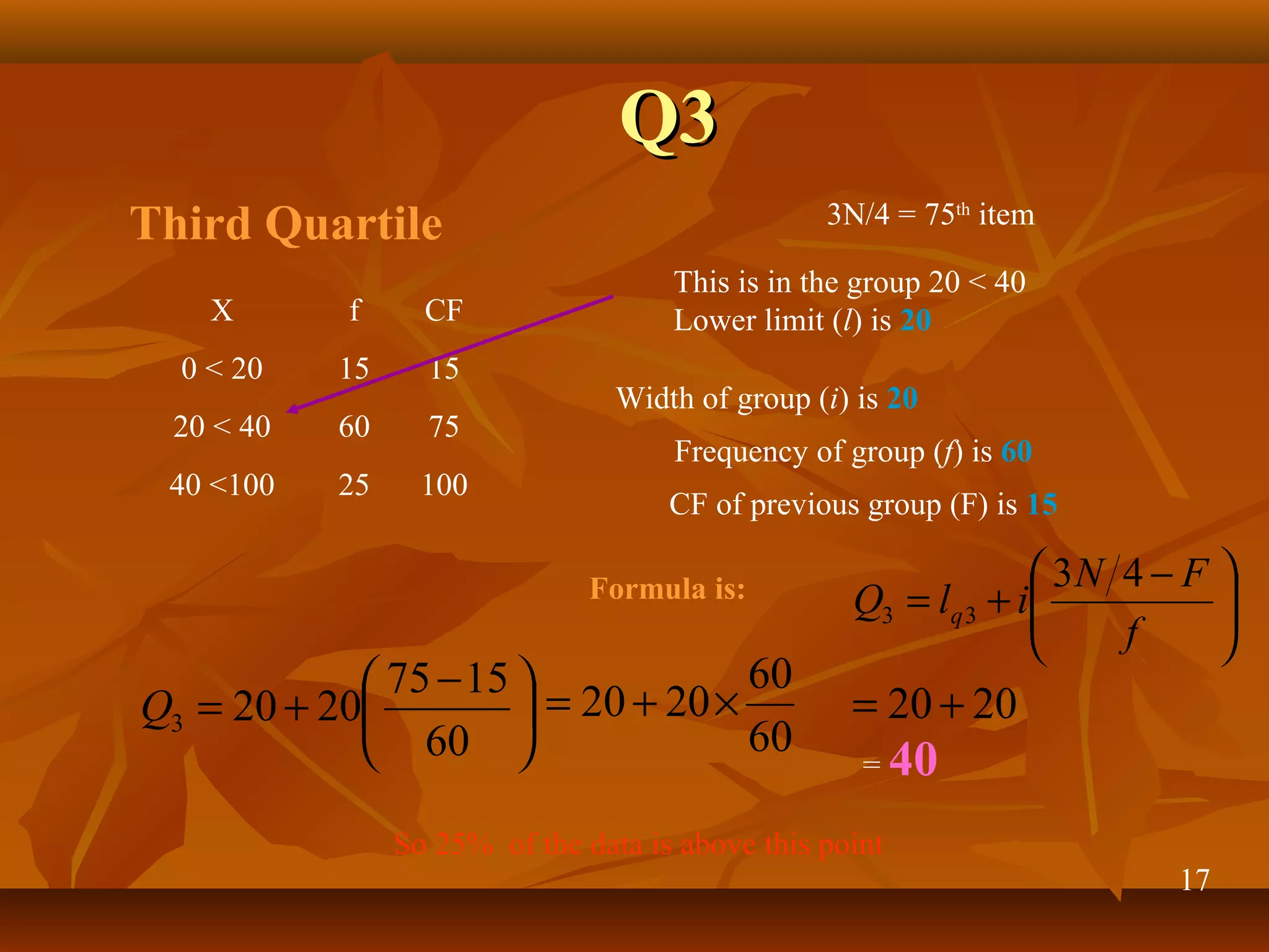
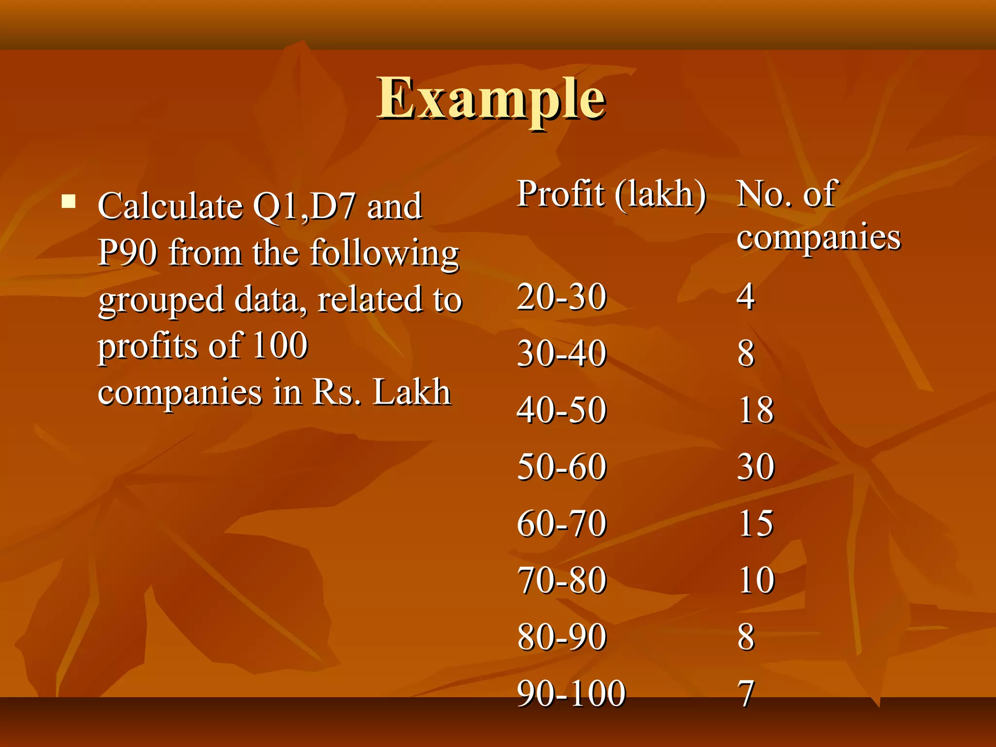
Definition and calculation of quartiles, how they divide data, and importance for data analysis.
Understanding percentiles, deciles, and their calculations in data distributions.


