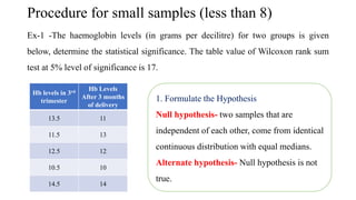
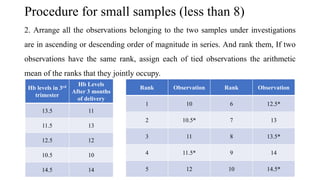
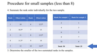
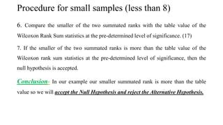
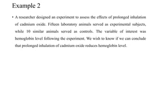
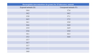
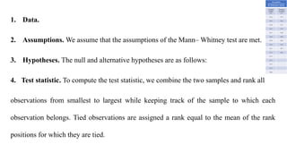
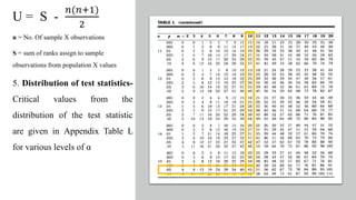
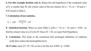
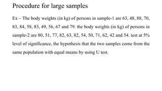
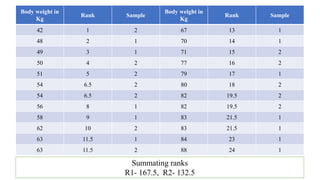
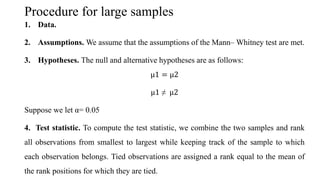
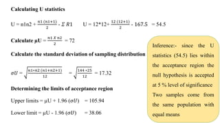
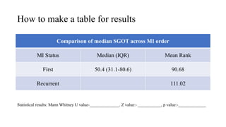
Mann Whitney
U Test
History of Mann Whitney U test
• 1892-1965 -Frank Wilcoxon (American
chemist and statistician)- for equal
sample size he proposed- Wilcoxon rank
sum test
• 1947 -extended to arbitrary sample size
• 1905-2000 -Henry Berthold Mann
(Austrian born American mathematician).
• 1915-2001 -Donald Ransom Whitney
(American statistician)
• 1892-1965 -Frank Wilcoxon (American
chemist and statistician)- for equal
sample size he proposed- Wilcoxon rank
sum test
• 1947 -extended to arbitrary sample size
• 1905-2000 -Henry Berthold Mann
(Austrian born American mathematician).
• 1915-2001 -Donald Ransom Whitney
(American statistician)
Assumption
• Two samples have been independently and randomly
drawn from their respective population.
• The scale of measurement is at least Ordinal.
• The variable of interest is continuous.
• The samples are identical and are proper
representative of population.
Procedure for small samples (less than 8)
Ex-1 -The haemoglobin levels (in grams per decilitre) for two groups is given
below, determine the statistical significance. The table value of Wilcoxon rank sum
test at 5% level of significance is 17.
Hb levels in 3rd
trimester
Hb Levels
After 3 months
of delivery
13.5 11
11.5 13
12.5 12
10.5 10
14.5 14
1. Formulate the Hypothesis
Null hypothesis- two samples that are
independent of each other, come from identical
continuous distribution with equal medians.
Alternate hypothesis- Null hypothesis is not
true.
Procedure for small samples (less than 8)
2. Arrange all the observations belonging to the two samples under investigations
are in ascending or descending order of magnitude in series. And rank them, If two
observations have the same rank, assign each of tied observations the arithmetic
mean of the ranks that they jointly occupy.
Rank Observation Rank Observation
1 10 6 12.5*
2 10.5* 7 13
3 11 8 13.5*
4 11.5* 9 14
5 12 10 14.5*
Hb levels in 3rd
trimester
Hb Levels
After 3 months
of delivery
13.5 11
11.5 13
12.5 12
10.5 10
14.5 14
Procedure for small samples (less than 8)
4. Summate the rank order individually for the two sample.
5. Determine the smaller of the two summated ranks in the samples.
Rank Observation Rank Observation
1 10 6 12.5*
2 10.5* 7 13
3 11 8 13.5*
4 11.5* 9 14
5 12 10 14.5*
Rank for sample 1 Rank for sample 2
2 1
4 3
6 5
8 7
10 9
Total- 30 Total- 25
Procedure for small samples (less than 8)
6. Compare the smaller of the two summated ranks with the table value of the
Wilcoxon Rank Sum statistics at the pre-determined level of significance. (17)
7. If the smaller of the two summated ranks is more than the table value of the
Wilcoxon rank sum statistics at the pre-determined level of significance, then the
null hypothesis is accepted.
Conclusion- In our example our smaller summated rank is more than the table
value so we will accept the Null Hypothesis and reject the Alternative Hypothesis.
Example 2
• A researcher designed an experiment to assess the effects of prolonged inhalation
of cadmium oxide. Fifteen laboratory animals served as experimental subjects,
while 10 similar animals served as controls. The variable of interest was
hemoglobin level following the experiment. We wish to know if we can conclude
that prolonged inhalation of cadmium oxide reduces hemoglobin level.
Haemoglobin determinations (in grams) for 25 laboratory animals
Exposed animals (X) Unexposed animals (Y)
14.4 17.4
14.2 16.2
13.8 17.1
16.5 17.5
14.1 15.0
16.6 16.0
15.9 16.9
15.6 15.0
14.1 16.3
15.3 16.8
15.7
16.7
13.7
15.3
14.0
1. Data.
2. Assumptions. We assume that the assumptions of the Mann– Whitney test are met.
3. Hypotheses. The null and alternative hypotheses are as follows:
4. Test statistic. To compute the test statistic, we combine the two samples and rank all
observations from smallest to largest while keeping track of the sample to which each
observation belongs. Tied observations are assigned a rank equal to the mean of the rank
positions for which they are tied.
Haemoglobin
determinations (in grams)
for 25 laboratory animals
Exposed
animals
(X)
Unexpose
d animals
(Y)
14.4 17.4
14.2 16.2
13.8 17.1
16.5 17.5
14.1 15.0
16.6 16.0
15.9 16.9
15.6 15.0
14.1 16.3
15.3 16.8
15.7
16.7
13.7
15.3
14.0
U = S -
𝑛(𝑛+1)
2
n = No. Of sample X observations
S = sum of ranks assign to sample
observations from population X values
5. Distribution of test statistics-
Critical values from the
distribution of the test statistic
are given in Appendix Table L
for various levels of α
6. For this example decision rule is- Reject the null hypothesis if the computed value
of U is smaller than 45, the critical value of the test statistic for n = 15, m = 10 and α =
0.05 found in Table L.
7. Calculation of test statistics.
U = 145 -
15(15+1)
2
=25
8. Statistical decision. When we enter Table L with n = 15, m = 10, and α = 0.05, we
find the critical value wα of to be 45. Since 25 < 45, we reject Null Hypothesis
9. Conclusion. This leads to the conclusion that prolonged inhalation of cadmium
oxide does reduce the haemoglobin level.
10. P value: since 22< 25 <30, we have for this test. 0.005> p > 0.001
Procedure for large samples
Ex – The body weights (in kg) of persons in sample-1 are 63, 48, 88, 70,
83, 84, 58, 83, 49, 56, 67 and 79. the body weights (in kg) of persons in
sample-2 are 80, 51, 77, 82, 63, 82, 54, 50, 71, 62, 42 and 54. test at 5%
level of significance, the hypothesis that the two samples come from the
same population with equal means by using U test.
Body weight in
Kg
Rank Sample
Body weight in
Kg
Rank Sample
42 1 2 67 13 1
48 2 1 70 14 1
49 3 1 71 15 2
50 4 2 77 16 2
51 5 2 79 17 1
54 6.5 2 80 18 2
54 6.5 2 82 19.5 2
56 8 1 82 19.5 2
58 9 1 83 21.5 1
62 10 2 83 21.5 1
63 11.5 1 84 23 1
63 11.5 2 88 24 1
Summating ranks
R1- 167.5, R2- 132.5
Procedure for large samples
1. Data.
2. Assumptions. We assume that the assumptions of the Mann– Whitney test are met.
3. Hypotheses. The null and alternative hypotheses are as follows:
µ1 = µ2
µ1 ≠ µ2
Suppose we let α= 0.05
4. Test statistic. To compute the test statistic, we combine the two samples and rank
all observations from smallest to largest while keeping track of the sample to which
each observation belongs. Tied observations are assigned a rank equal to the mean of
the rank positions for which they are tied.
Calculating U statistics
U = n1n2 +
𝑛1 (𝑛1+1)
2
- 𝛴 𝑅1 U = 12*12+
12 (12+1)
2
- 167.5 = 54.5
Calculate µU =
𝑛1 𝑋 𝑛2
2
= 72
Calculate the standard deviation of sampling distribution
𝜎𝑈 =
𝑛1∗𝑛2 (𝑛1+𝑛2+1)
12
=
144 ∗25
12
= 17.32
Determining the limits of acceptance region
Upper limits = µU + 1.96 (𝜎𝑈) = 105.94
Lower limit = µU - 1.96 (𝜎𝑈) = 38.06
Inference:- since the U
statistics (54.5) lies within
the acceptance region the
null hypothesis is accepted
at 5 % level of significance
Two samples come from
the same population with
equal means
How to make a table for results
Comparison of median SGOT across MI order
MI Status Median (IQR) Mean Rank
First 50.4 (31.1-80.6) 90.68
Recurrent 111.02
Statistical results: Mann Whitney U value-______________. Z value:- ___________, p value:-_____________

Non parametric test- MANN WHITNEY U TEST.pptx

  • 1.
  • 2.
    History of MannWhitney U test • 1892-1965 -Frank Wilcoxon (American chemist and statistician)- for equal sample size he proposed- Wilcoxon rank sum test • 1947 -extended to arbitrary sample size • 1905-2000 -Henry Berthold Mann (Austrian born American mathematician). • 1915-2001 -Donald Ransom Whitney (American statistician) • 1892-1965 -Frank Wilcoxon (American chemist and statistician)- for equal sample size he proposed- Wilcoxon rank sum test • 1947 -extended to arbitrary sample size • 1905-2000 -Henry Berthold Mann (Austrian born American mathematician). • 1915-2001 -Donald Ransom Whitney (American statistician)
  • 3.
    Assumption • Two sampleshave been independently and randomly drawn from their respective population. • The scale of measurement is at least Ordinal. • The variable of interest is continuous. • The samples are identical and are proper representative of population.
  • 4.
    Procedure for smallsamples (less than 8) Ex-1 -The haemoglobin levels (in grams per decilitre) for two groups is given below, determine the statistical significance. The table value of Wilcoxon rank sum test at 5% level of significance is 17. Hb levels in 3rd trimester Hb Levels After 3 months of delivery 13.5 11 11.5 13 12.5 12 10.5 10 14.5 14 1. Formulate the Hypothesis Null hypothesis- two samples that are independent of each other, come from identical continuous distribution with equal medians. Alternate hypothesis- Null hypothesis is not true.
  • 5.
    Procedure for smallsamples (less than 8) 2. Arrange all the observations belonging to the two samples under investigations are in ascending or descending order of magnitude in series. And rank them, If two observations have the same rank, assign each of tied observations the arithmetic mean of the ranks that they jointly occupy. Rank Observation Rank Observation 1 10 6 12.5* 2 10.5* 7 13 3 11 8 13.5* 4 11.5* 9 14 5 12 10 14.5* Hb levels in 3rd trimester Hb Levels After 3 months of delivery 13.5 11 11.5 13 12.5 12 10.5 10 14.5 14
  • 6.
    Procedure for smallsamples (less than 8) 4. Summate the rank order individually for the two sample. 5. Determine the smaller of the two summated ranks in the samples. Rank Observation Rank Observation 1 10 6 12.5* 2 10.5* 7 13 3 11 8 13.5* 4 11.5* 9 14 5 12 10 14.5* Rank for sample 1 Rank for sample 2 2 1 4 3 6 5 8 7 10 9 Total- 30 Total- 25
  • 7.
    Procedure for smallsamples (less than 8) 6. Compare the smaller of the two summated ranks with the table value of the Wilcoxon Rank Sum statistics at the pre-determined level of significance. (17) 7. If the smaller of the two summated ranks is more than the table value of the Wilcoxon rank sum statistics at the pre-determined level of significance, then the null hypothesis is accepted. Conclusion- In our example our smaller summated rank is more than the table value so we will accept the Null Hypothesis and reject the Alternative Hypothesis.
  • 8.
    Example 2 • Aresearcher designed an experiment to assess the effects of prolonged inhalation of cadmium oxide. Fifteen laboratory animals served as experimental subjects, while 10 similar animals served as controls. The variable of interest was hemoglobin level following the experiment. We wish to know if we can conclude that prolonged inhalation of cadmium oxide reduces hemoglobin level.
  • 9.
    Haemoglobin determinations (ingrams) for 25 laboratory animals Exposed animals (X) Unexposed animals (Y) 14.4 17.4 14.2 16.2 13.8 17.1 16.5 17.5 14.1 15.0 16.6 16.0 15.9 16.9 15.6 15.0 14.1 16.3 15.3 16.8 15.7 16.7 13.7 15.3 14.0
  • 10.
    1. Data. 2. Assumptions.We assume that the assumptions of the Mann– Whitney test are met. 3. Hypotheses. The null and alternative hypotheses are as follows: 4. Test statistic. To compute the test statistic, we combine the two samples and rank all observations from smallest to largest while keeping track of the sample to which each observation belongs. Tied observations are assigned a rank equal to the mean of the rank positions for which they are tied. Haemoglobin determinations (in grams) for 25 laboratory animals Exposed animals (X) Unexpose d animals (Y) 14.4 17.4 14.2 16.2 13.8 17.1 16.5 17.5 14.1 15.0 16.6 16.0 15.9 16.9 15.6 15.0 14.1 16.3 15.3 16.8 15.7 16.7 13.7 15.3 14.0
  • 11.
    U = S- 𝑛(𝑛+1) 2 n = No. Of sample X observations S = sum of ranks assign to sample observations from population X values 5. Distribution of test statistics- Critical values from the distribution of the test statistic are given in Appendix Table L for various levels of α
  • 12.
    6. For thisexample decision rule is- Reject the null hypothesis if the computed value of U is smaller than 45, the critical value of the test statistic for n = 15, m = 10 and α = 0.05 found in Table L. 7. Calculation of test statistics. U = 145 - 15(15+1) 2 =25 8. Statistical decision. When we enter Table L with n = 15, m = 10, and α = 0.05, we find the critical value wα of to be 45. Since 25 < 45, we reject Null Hypothesis 9. Conclusion. This leads to the conclusion that prolonged inhalation of cadmium oxide does reduce the haemoglobin level. 10. P value: since 22< 25 <30, we have for this test. 0.005> p > 0.001
  • 13.
    Procedure for largesamples Ex – The body weights (in kg) of persons in sample-1 are 63, 48, 88, 70, 83, 84, 58, 83, 49, 56, 67 and 79. the body weights (in kg) of persons in sample-2 are 80, 51, 77, 82, 63, 82, 54, 50, 71, 62, 42 and 54. test at 5% level of significance, the hypothesis that the two samples come from the same population with equal means by using U test.
  • 14.
    Body weight in Kg RankSample Body weight in Kg Rank Sample 42 1 2 67 13 1 48 2 1 70 14 1 49 3 1 71 15 2 50 4 2 77 16 2 51 5 2 79 17 1 54 6.5 2 80 18 2 54 6.5 2 82 19.5 2 56 8 1 82 19.5 2 58 9 1 83 21.5 1 62 10 2 83 21.5 1 63 11.5 1 84 23 1 63 11.5 2 88 24 1 Summating ranks R1- 167.5, R2- 132.5
  • 15.
    Procedure for largesamples 1. Data. 2. Assumptions. We assume that the assumptions of the Mann– Whitney test are met. 3. Hypotheses. The null and alternative hypotheses are as follows: µ1 = µ2 µ1 ≠ µ2 Suppose we let α= 0.05 4. Test statistic. To compute the test statistic, we combine the two samples and rank all observations from smallest to largest while keeping track of the sample to which each observation belongs. Tied observations are assigned a rank equal to the mean of the rank positions for which they are tied.
  • 16.
    Calculating U statistics U= n1n2 + 𝑛1 (𝑛1+1) 2 - 𝛴 𝑅1 U = 12*12+ 12 (12+1) 2 - 167.5 = 54.5 Calculate µU = 𝑛1 𝑋 𝑛2 2 = 72 Calculate the standard deviation of sampling distribution 𝜎𝑈 = 𝑛1∗𝑛2 (𝑛1+𝑛2+1) 12 = 144 ∗25 12 = 17.32 Determining the limits of acceptance region Upper limits = µU + 1.96 (𝜎𝑈) = 105.94 Lower limit = µU - 1.96 (𝜎𝑈) = 38.06 Inference:- since the U statistics (54.5) lies within the acceptance region the null hypothesis is accepted at 5 % level of significance Two samples come from the same population with equal means
  • 17.
    How to makea table for results Comparison of median SGOT across MI order MI Status Median (IQR) Mean Rank First 50.4 (31.1-80.6) 90.68 Recurrent 111.02 Statistical results: Mann Whitney U value-______________. Z value:- ___________, p value:-_____________