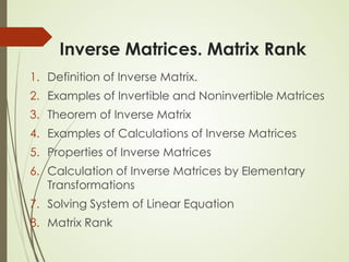
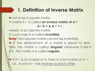
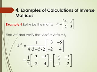
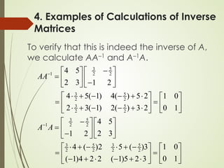
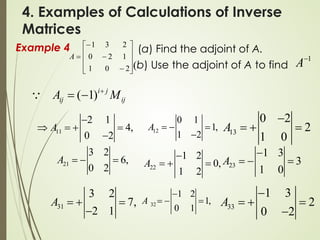
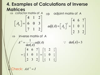
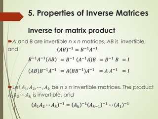
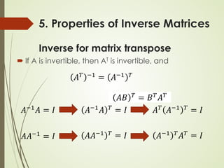
This lecture discusses inverse matrices and matrix rank. It defines an inverse matrix as a matrix A-1 such that A-1A = AA-1 = I, where I is the identity matrix. For a matrix to have an inverse, it must be square and have a non-zero determinant. The lecture provides examples of calculating inverse matrices and shows that the inverse can be found using the adjoint matrix and determinant. Properties of inverse matrices include the inverse of products and transposes. Inverse matrices can also be computed using Gaussian elimination to put the matrix in reduced row echelon form. Matrix rank is also introduced.

1. Lecture № 3
Inverse Matrices.
Matrix Rank
Senior lecturer Marina Hotomceva

2. Inverse Matrices. Matrix Rank
1. Definition of Inverse Matrix.
2. Examples of Invertible and Noninvertible Matrices
3. Theorem of Inverse Matrix
4. Examples of Calculations of Inverse Matrices
5. Properties of Inverse Matrices
6. Calculation of Inverse Matrices by Elementary
Transformations
7. Solving System of Linear Equation
8. Matrix Rank

3. 1. Definition of Inverse Matrix
 Let A be a square matrix.
A matrix A−¹ is called an inverse matrix of A if
A−¹A = A A−¹ = I ,
where I is an identity matrix.
In such case A is called invertible.
Note: Non-square matrix cannot be invertible.
 If the determinant of a matrix is equal to zero,
then the matrix is called singular; otherwise, if det A
≠ 0 , the matrix A is called regular.
 If A−¹ is an inverse of A, then A is an inverse of A−¹,
i.e., A and A−¹ are inverses to each other.

4. 2. Examples of Invertible and
Noninvertible Matrices
 Example 1 B is an inverse of A.
𝐴𝐴 =
2 1
5 3
𝐵𝐵 =
3 −1
−5 2
So, A is invertible and B=A−¹
𝐴𝐴𝐴𝐴 =
2 1
5 3
3 −1
−5 2
=
2 ⋅ 3 + 1 −5 2 −1 + 1 ⋅ 2
5 ⋅ 3 + 3 −5 5 −1 + 3 ⋅ 2
=
1 0
0 1
𝐵𝐵𝐵𝐵 =
3 −1
−5 2
2 1
5 3
=
3 ⋅ 2 + −1 5 3 ⋅ 1 + −1 3
−5 2 + 2 ⋅ 5 −5 1 + 2 ⋅ 3
=
1 0
0 1

5. 2. Examples of Invertible and
Noninvertible Matrices
 Example 2. Not all the square matrix is invertible

6. 3. Theorem of Inverse Matrix
 If each element of a square matrix A is replaced by
its cofactor, then the transpose of the matrix
obtained is called the adjoint matrix of A:
Matrix of cofactors of A:
Adjoint matrix of A:
[ ]
11 12 1
21 22 2
1 2
n
n
ij
n n nn
A A A
A A A
A
A A A
 
 
 
=
 
 
 


  

11 21 1
12 22 2
1 2
( )
n
T n
ij
n n nn
A A A
A A A
adj A A
A A A
 
 
 
 
= =
   
 
 


  


7. 3. Theorem of Inverse Matrix
For any regular matrix A there exists the unique inverse
matrix:
Any singular matrix has no an inverse matrix.
( )
1 1
adj
det
A A
A
−
=

8. 4. Examples of Calculations of Inverse
Matrices
Example 3. Given the matrix find the inverse
of A
,
a b
A
c d
 
=  
 
bc
ad
A −
=
⇒ )
det( 





−
−
=
a
c
b
d
A
adj )
(
( )
)
(
det
1
1
A
adj
A
A =
⇒ −






−
−
−
=
a
c
b
d
bc
ad
1

9. 4. Examples of Calculations of Inverse
Matrices
Example 4 Let A be the matrix
Find A–1 and verify that AA–1 = A–1A = I2
4 5
2 3
A
 
=  
 
1
3 5
2 2
3 5
1
2 4
4 3 5 2
3 5
1
2 4 1 2
2
A− −
 
=  
−
⋅ − ⋅  
− −
 
 
= =  
 
− −
   

10. To verify that this is indeed the inverse of A,
we calculate AA–1 and A–1A.
4. Examples of Calculations of Inverse
Matrices
3 5
1 2 2
3 5
2 2
3 5
2 2
3 5
1 2 2
3 5 3 5
2 2 2 2
4 5
2 3 1 2
4 5( 1) 4( ) 5 2 1 0
2 3( 1) 2( ) 3 2 0 1
4 5
2 3
1 2
1 0
4 ( )2 5 ( )3
0 1
( 1)4 2 2 ( 1)5 2 3
AA
A A
−
−
−
 
 
=  
  −
   
⋅ + − − + ⋅
   
=
   
⋅ + − − + ⋅  
 
−
   
=    
−  
 
⋅ + − ⋅ + −
   
=
   
− + ⋅ − + ⋅  
 

11. 4. Examples of Calculations of Inverse
Matrices
Example 4
1
−
A










−
−
−
=
2
0
1
1
2
0
2
3
1
A
(a) Find the adjoint of A.
(b) Use the adjoint of A to find
11
2 1
4,
0 2
A
−
⇒ =
+ =
−
12
0 1
1,
1 2
A =
− =
− 13
0 2
2
1 0
A
−
=
+ =
( 1)i j
ij ij
A M
+
= −

21
3 2
6,
0 2
A =
− =
22
1 2
0,
1 2
A
−
=
+ =
23
1 3
3
1 0
A
−
=
− =
31
3 2
7,
2 1
A =
+ =
−
32
1 2
1,
0 1
A
−
=
− =
33
1 3
2
0 2
A
−
=
+ =
−

12. 4. Examples of Calculations of Inverse
Matrices
cofactor matrix of A
⇒
4 1 2
6 0 3
7 1 2
ij
A
 
 
  =
   
 
 
adjoint matrix of A
⇒
4 6 7
( ) 1 0 1
2 3 2
T
ij
adj A A
 
 
 
= =
   
 
 










=
2
3
2
1
0
1
7
6
4
3
1
⇒ inverse matrix of A
( )
)
(
det
1
1
A
adj
A
A =
−
( ) 3
det =
A











=
3
2
3
2
3
1
3
1
3
7
3
4
1
0
2
 Check: I
AA =
−1

13. 5. Properties of Inverse Matrices
Inverse for matrix product
A and B are invertible n x n matrices, AB is invertible,
and
Let 𝐴𝐴1, 𝐴𝐴2, ⋯ , 𝐴𝐴𝑘𝑘 be n x n invertible matrices. The product
𝐴𝐴1𝐴𝐴2 ⋯ 𝐴𝐴𝑘𝑘 is invertible, and
𝐴𝐴𝐴𝐴 −1 = 𝐵𝐵−1𝐴𝐴−1
𝐵𝐵−1𝐴𝐴−1 𝐴𝐴𝐴𝐴 = 𝐵𝐵−1 𝐴𝐴−1𝐴𝐴 𝐵𝐵 = 𝐵𝐵−1 𝐵𝐵 = 𝐼𝐼
𝐴𝐴𝐴𝐴 𝐵𝐵−1𝐴𝐴−1 = 𝐴𝐴 𝐵𝐵𝐵𝐵−1 𝐴𝐴−1 = 𝐴𝐴 𝐴𝐴−1 = 𝐼𝐼
𝐴𝐴1𝐴𝐴2 ⋯ 𝐴𝐴𝑘𝑘
−1
= 𝐴𝐴𝑘𝑘
−1
𝐴𝐴𝑘𝑘−1
−1
⋯ 𝐴𝐴1
−1

14. 5. Properties of Inverse Matrices
Inverse for matrix transpose
 If A is invertible, then AT is invertible, and
𝐴𝐴−1
𝐴𝐴 = 𝐼𝐼
𝐴𝐴𝐴𝐴−1 = 𝐼𝐼
𝐴𝐴𝐴𝐴 𝑇𝑇 = 𝐵𝐵𝑇𝑇𝐴𝐴𝑇𝑇
𝐴𝐴−1𝐴𝐴 𝑇𝑇 = 𝐼𝐼
𝐴𝐴𝐴𝐴−1 𝑇𝑇 = 𝐼𝐼
𝐴𝐴𝑇𝑇
𝐴𝐴−1 𝑇𝑇
= 𝐼𝐼
𝐴𝐴𝑇𝑇 −1 = 𝐴𝐴−1 𝑇𝑇
𝐴𝐴−1 𝑇𝑇𝐴𝐴𝑇𝑇 = 𝐼𝐼

15. 7.Calculation of Inverse Matrices
by Elementary Transformations
 Reduced Row Echelon Form
1. If a row does not consist entirely of zeros, then the first nonzero number
in the row is a 1. We call this a leading 1.
2. If there are any rows that consist entirely of zeros, then they are
grouped together at the bottom of the matrix.
3. In any two successive rows that do not consist entirely of zeros, the
leading 1 in the lower row occurs farther to the right than the leading 1 in
the higher row.
4. Each column that contains a leading 1 has zeros everywhere else in
that column.
1. Each nonzero row lies above every zero row
2. The leading entries are in echelon form

16. 7.Calculation of Inverse Matrices by
Elementary Transformations
 Reduced Row Echelon Form (RREF)
No zero rows

17. 7.Calculation of Inverse Matrices
by Elementary Transformations
 Reduced Row Echelon Form (RREF)
1-2 The matrix is in row
echelon form
3. The columns
containing the leading
entries are standard
vectors.

18. 7.Calculation of Inverse Matrices
by Elementary Transformations
Gaussian Elimination
 Gaussian elimination: an algorithm for finding the reduced row
echelon form of a matrix.
Original
matrix
A row echelon
form
The reduced row
echelon form
forward pass backward pass
Elementary row
operations
Elementary row
operations

19. 7.Calculation of Inverse Matrices
by Elementary Transformations
elementary row operations
A ……
A’ A’’ R
1. Interchange any two rows of the matrix
2. Multiply every entry of some row by the same nonzero
scalar
3. Add a multiple of one row of the matrix to another row
Note: Every elementary row operations are reversible
reduced row echelon form

20. 7.Calculation of Inverse Matrices
by Elementary Transformations
1
-2
3
The pivot positions of A are (1,1),
Example 5 Reduce matrix to reduced row echelon form.

21. 7.Calculation of Inverse Matrices
by Elementary Transformations

22. -1
7.Calculation of Inverse Matrices
by Elementary Transformations

23. -2
7.Calculation of Inverse Matrices
by Elementary Transformations

24. 7.Calculation of Inverse Matrices
by Elementary Transformations

25. 7.Calculation of Inverse Matrices
by Elementary Transformations

26. 7.Calculation of Inverse Matrices by
Elementary Transformations

27. 7.Calculation of Inverse Matrices
by Elementary Transformations
Elementary Row Operation
Every elementary row operation can be performed by
matrix multiplication.
 1. Interchange
 2. Scaling
 3. Adding k times row i to row j:
0
0
1
1
1
k
0
0
1
1
k
0

28. 7.Calculation of Inverse Matrices
by Elementary Transformations
 Every elementary row operation can be performed by
matrix multiplication.
 How to find elementary matrix?
𝐸𝐸
1 0 0
0 1 0
0 0 1
E.g. the elementary matrix that exchange the 1st
and 2nd rows
0 1 0
1 0 0
0 0 1
=
𝐸𝐸
1 4
2 5
3 6
=
2 5
1 4
3 6
𝐸𝐸 =
0 1 0
1 0 0
0 0 1

29. 7.Calculation of Inverse Matrices
by Elementary Transformations
 How to find elementary matrix?
 Apply the desired elementary row operation on
Identity matrix
𝐸𝐸1 =
1 0 0
0 0 1
0 1 0
𝐸𝐸2 =
1 0 0
0 −4 0
0 0 1
𝐸𝐸3 =
1 0 0
0 1 0
2 0 1
Exchange the
2nd and 3rd
rows
Multiply the
2nd row by -4
Adding 2
times row 1 to
row 3
1 0 0
0 1 0
0 0 1
1 0 0
0 1 0
0 0 1
1 0 0
0 1 0
0 0 1

30. 7.Calculation of Inverse Matrices
by Elementary Transformations
 How to find elementary matrix?
 Apply the desired elementary row operation on
Identity matrix
𝐸𝐸1 =
1 0 0
0 0 1
0 1 0
𝐸𝐸2 =
1 0 0
0 −4 0
0 0 1
𝐸𝐸3 =
1 0 0
0 1 0
2 0 1
𝐴𝐴 =
1 4
2 5
3 6
𝐸𝐸1𝐴𝐴 =
1 4
3 6
2 5
𝐸𝐸2𝐴𝐴 =
1 4
−8 −20
3 6
𝐸𝐸3𝐴𝐴 =
1 4
2 5
5 14

31. 7.Calculation of Inverse Matrices
by Elementary Transformations
The inverse of elementary matrix is another
elementary matrix that do the reverse row operation.

32. 𝐸𝐸1 =
1 0 0
0 0 1
0 1 0
𝐸𝐸2 =
1 0 0
0 −4 0
0 0 1
𝐸𝐸3 =
1 0 0
0 1 0
2 0 1
Exchange the 2nd and 3rd
rows
Multiply the 2nd row by
-4
Adding 2 times row 1 to
row 3
Exchange the 2nd and 3rd
rows
𝐸𝐸1
−1
=
1 0 0
0 0 1
0 1 0
Multiply the 2nd row by -1/4
𝐸𝐸2
−1
=
1 0 0
0 −1/4 0
0 0 1
Adding -2 times row 1 to
row 3
𝐸𝐸3
−1
=
1 0 0
0 1 0
−2 0 1
Reverse elementary row operation

33. 7.Calculation of Inverse Matrices by
Elementary Transformations
RREF versus Elementary Matrix
 Let A be a n x n matrix with reduced row echelon form
R.
 There exists an invertible n x n matrix P such that PA=R
𝐸𝐸𝑘𝑘 ⋯ 𝐸𝐸2𝐸𝐸1𝐴𝐴 = 𝑅𝑅
𝑃𝑃 = 𝐸𝐸𝑘𝑘 ⋯ 𝐸𝐸2𝐸𝐸1
𝑃𝑃−1
= 𝐸𝐸1
−1
𝐸𝐸2
−1
⋯ 𝐸𝐸𝑘𝑘
−1

34. 7.Calculation of Inverse Matrices by
Elementary Transformations
Invertible
Let A be an n x n matrix. A is invertible if and only if
The reduced row echelon form of A is In
In
Invertible
Not Invertible
RREF
RREF

35. 7.Calculation of Inverse Matrices
by Elementary Transformations
Invertible
The reduced row
echelon form of A is In
A is a product of
elementary matrices
An n x n matrix A is
invertible. R=RREF(A)=In
𝐸𝐸𝑘𝑘 ⋯ 𝐸𝐸2𝐸𝐸1𝐴𝐴 = 𝐼𝐼𝑛𝑛
𝐴𝐴 = 𝐸𝐸1
−1
𝐸𝐸2
−1
⋯ 𝐸𝐸𝑘𝑘
−1
𝐼𝐼𝑛𝑛
= 𝐸𝐸1
−1
𝐸𝐸2
−1
⋯ 𝐸𝐸𝑘𝑘
−1

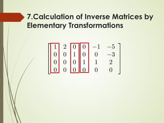
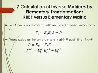
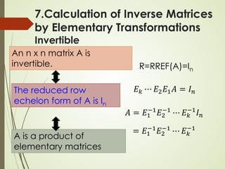
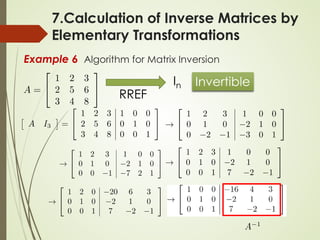
36. Algorithm for Matrix Inversion
 Let A be an n x n matrix. Transform [ A In ] into its RREF
[ R B ]
R is the RREF of A
B is a n x n matrix (not RREF)
 If R = In, then A is invertible B = A-1
𝐸𝐸𝑘𝑘 ⋯ 𝐸𝐸2𝐸𝐸1 𝐴𝐴 𝐼𝐼𝑛𝑛 = 𝑅𝑅 𝐸𝐸𝑘𝑘 ⋯ 𝐸𝐸2𝐸𝐸1
𝐴𝐴−1
𝐼𝐼𝑛𝑛
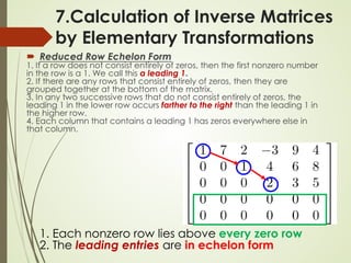
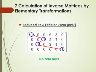
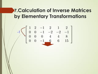
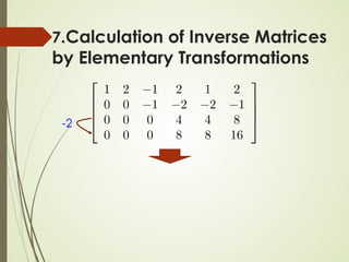
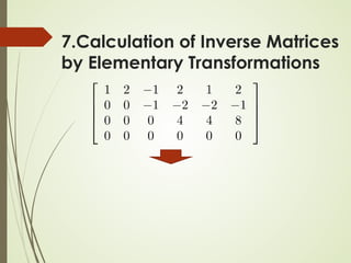
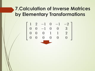
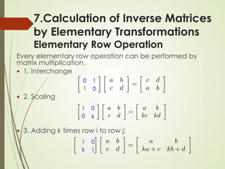
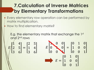
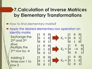
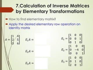
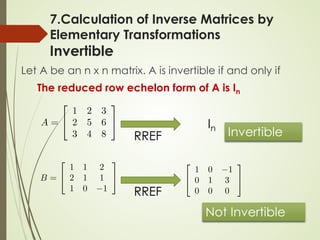
7.Calculation of Inverse Matrices
by Elementary Transformations

37. Example 6 Algorithm for Matrix Inversion
In Invertible
RREF
7.Calculation of Inverse Matrices by
Elementary Transformations

38. 7. Solving System of Linear Equation
We solve this matrix equation by multiplying each
side by the inverse of A—provided the inverse exists.
AX = B
A–1(AX) = A–1B
(A–1A)X = A–1B Associative Property
I3X = A–1B Property of Inverse
X = A–1B
However, this method is computationally inefficient.

39. 7. Solving System of Linear Equation
Example 7 �
2𝑥𝑥 − 5𝑦𝑦 = 15
3𝑥𝑥 − 6𝑦𝑦 = 36
a) Write the system of equations as a matrix equation.
b) Solve the system by solving the matrix equation
Sol: We write the system as a matrix equation of the form
AX = B: 2 −5
3 −6
𝑥𝑥
𝑦𝑦 =
15
36
𝐴𝐴−1 =
2 −5
3 −6
−1
=
1
2 −6 − −5 3
−6 − −5
−3 2
=
1
3
−6 5
−3 2
=
−2
5
3
−1
2
3
𝑥𝑥
𝑦𝑦 =
−2
5
3
−1
2
3
15
36
=
30
9

40. 8. Matrix Rank
 An m x n matrix A is said to be the matrix of rank r, if
– there exists at least one regular submatrix of order r ;
– every submatrix of a higher order is singular.
 The rank of a matrix can be evaluated by applying
just those elementary transformation which are used
to reduce matrix to reduced row echelon form.
 If a row or column consists of zeros, then it can be
omitted.
 Theorem: If a matrix à is obtained from A by
elementary transformations then rank à = rank A .

41. Maximum number
of Independent
Columns
Number of Pivot
Column
=
=
Number of Non-zero
rows
Pivot
column
Leading
Entry
Non-
zero row
Rank = ?
Rank = ? 3
3

42. 8. Matrix Rank
Properties of Rank from RREF
Rank A ≤ Number of columns
Rank A ≤ Number of rows
Rank A ≤ Min( Number of
columns, Number of rows)
Number of Pivot
Column
=
=
Number of Non-zero
rows
Maximum number of
Independent
Columns

43. 8. Matrix Rank
Example 9. Find the rank of the matrix
This matrix is in reduced echelon form. There are three
nonzero row namely (1, 2, 0, 0), (0, 0, 1, 0), and (0, 0, 0,
1). Rank(A) = 3.










=
0
0
0
0
1
0
0
0
0
1
0
0
0
0
2
1
A

44. 8. Matrix Rank
Example 10. Given A. Determine its rank.
1 2 3
2 5 4
1 1 5
A
 
 
=  
 
 
Use elementary row operations to find a reduced
echelon form of the matrix A. We get
1 2 3 1 2 3 1 0 7
2 5 4 0 1 2 0 1 2
1 1 5 0 1 2 0 0 0
     
     
− −
     
     
−
     
 
Obtain two nonzero rows (1, 0, 7), (0, 1, -2) rows. Hence
rank(A) = 2.