Download to read offline
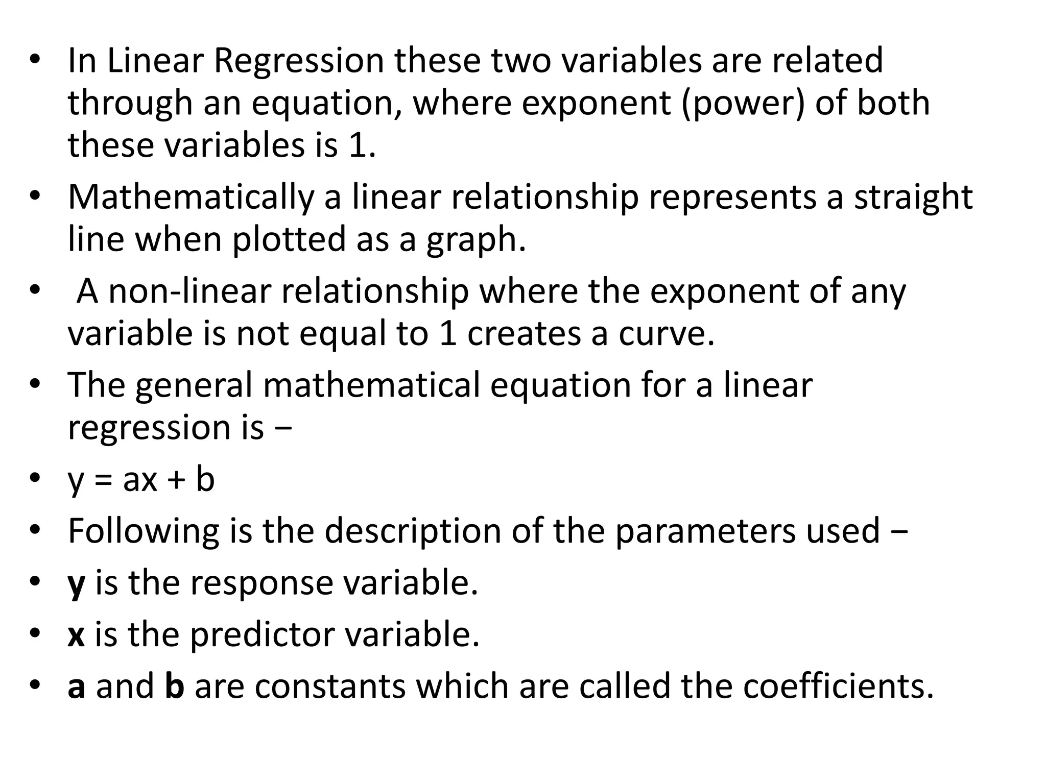

Linear regression establishes a relationship model between two variables, a predictor variable and a response variable. The relationship is represented by a linear equation where the exponent of both variables is 1, forming a straight line when graphed. Assumptions of linear regression include a linear relationship between variables, normally distributed residuals, and homoscedasticity. Linear regression is used to predict the response variable for new observations by fitting a linear model to observed data using functions like lm() and predict() in R.
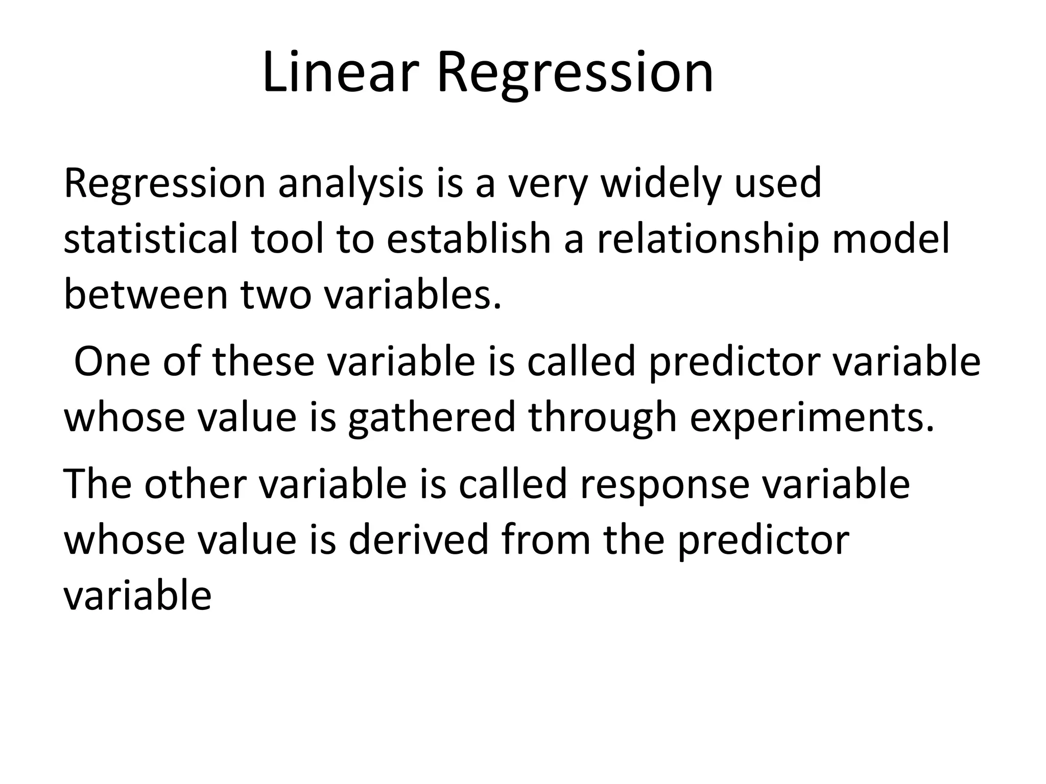
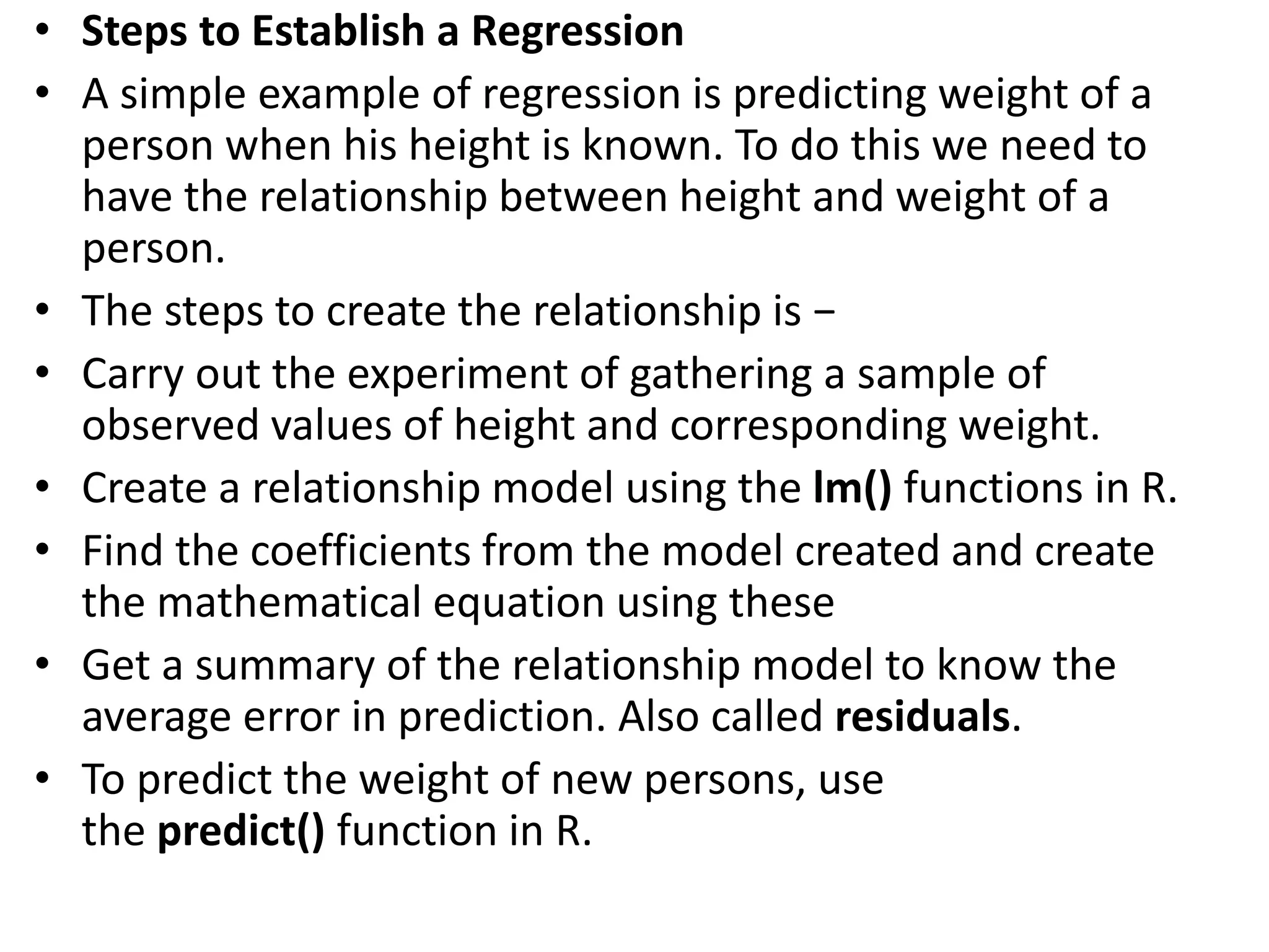
Introduction to regression analysis, its relationship model, and steps to establish a linear regression.
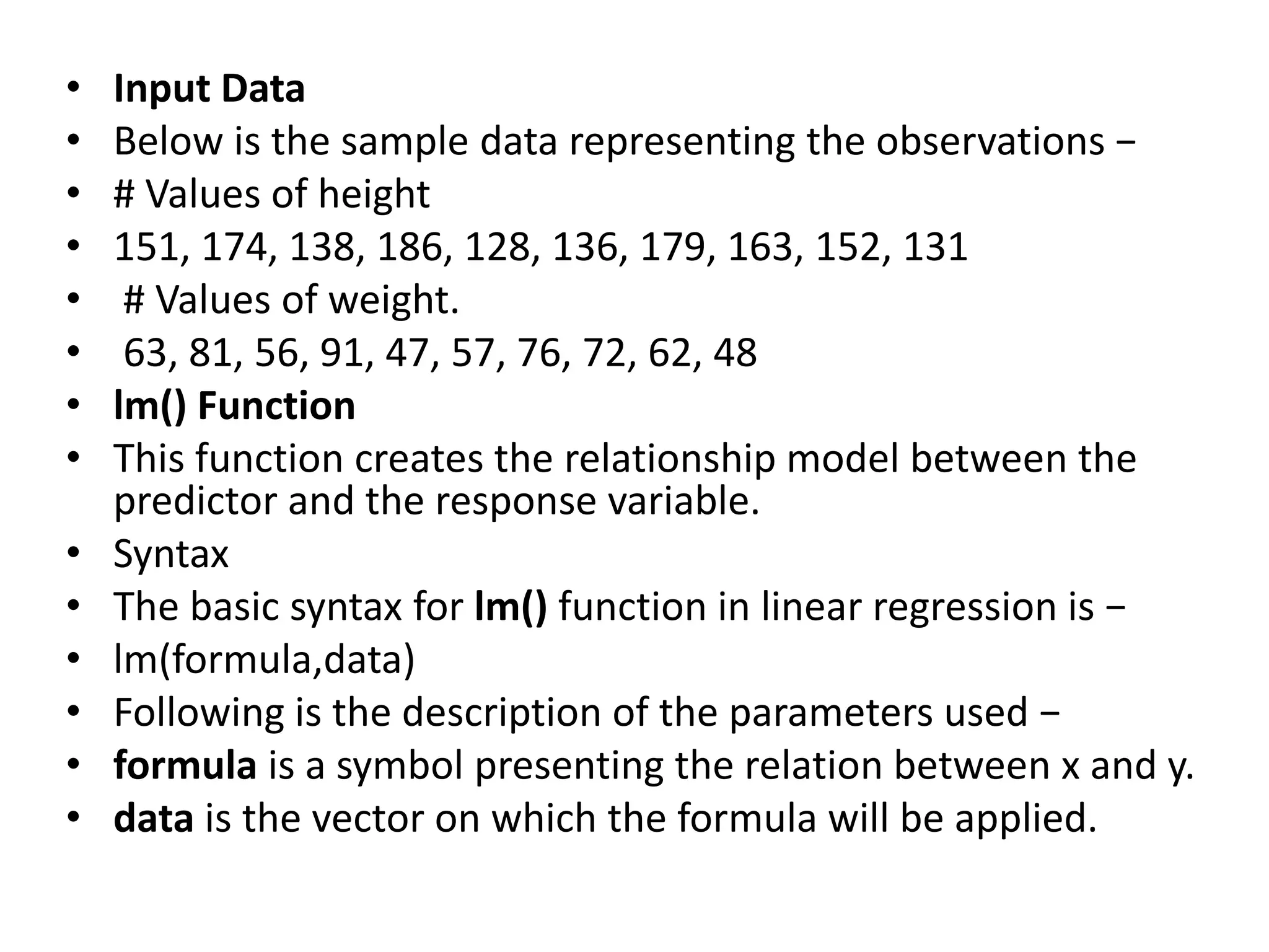
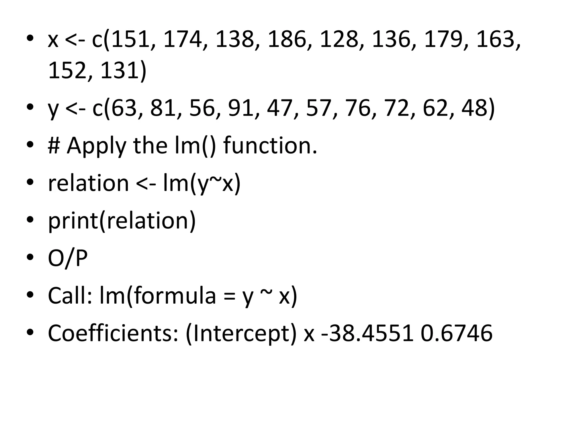
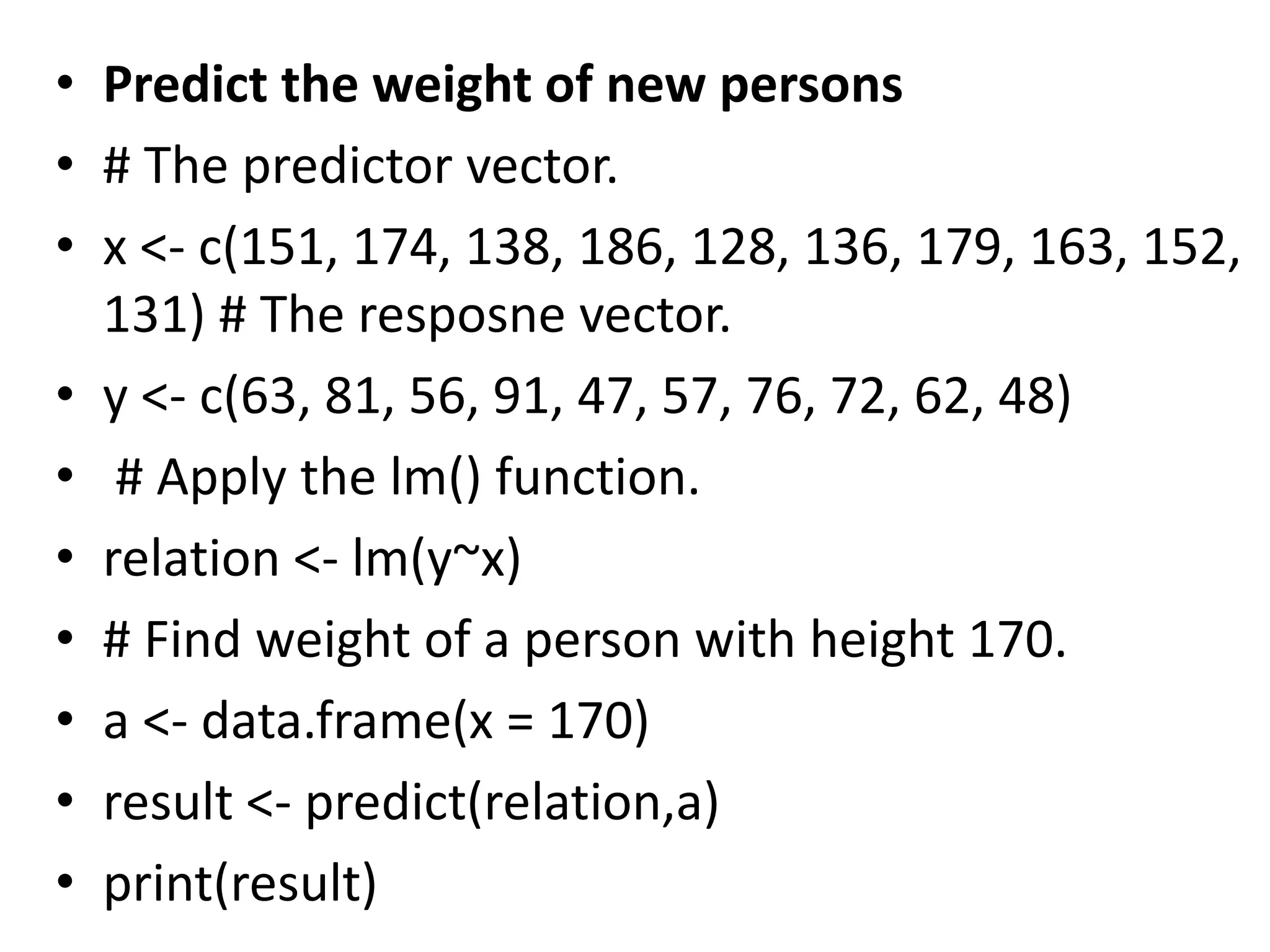
Overview of input data for height and weight, and the application of the lm() function to create a model.
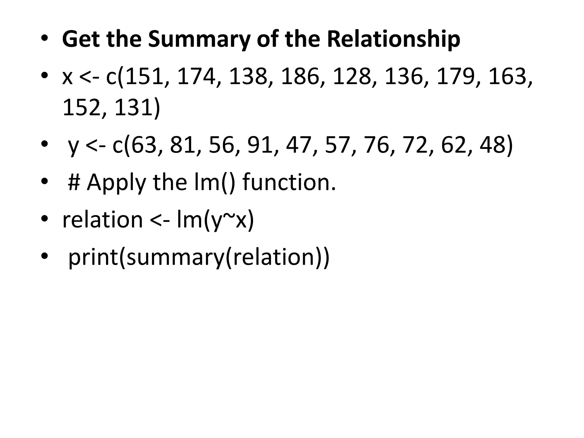
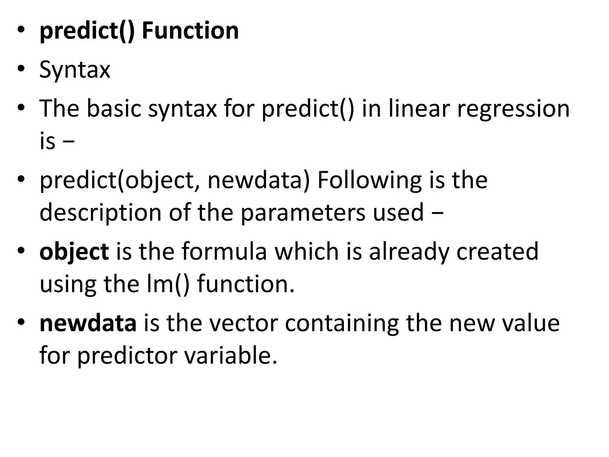
Using R to create a linear regression model, summarizing the relationship, and predicting new values.
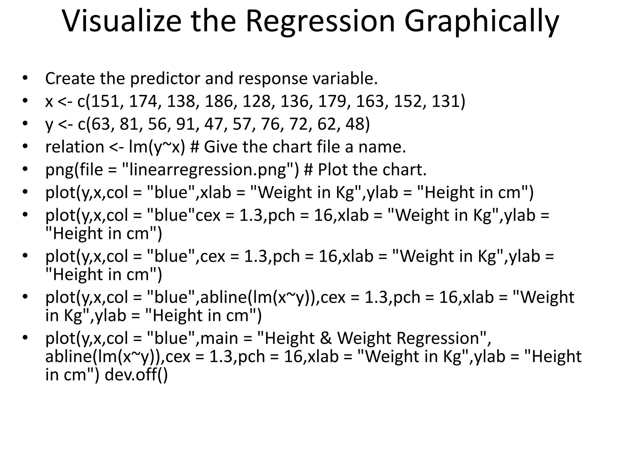
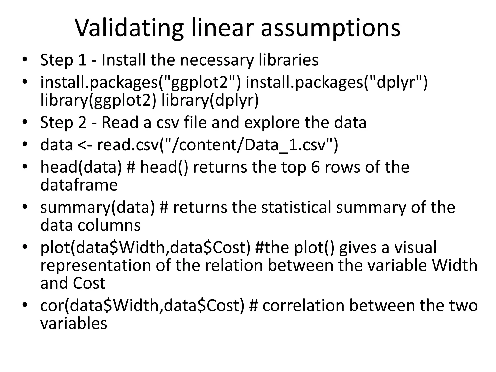
Instructions for visualizing linear regression data graphically, including plotting techniques.
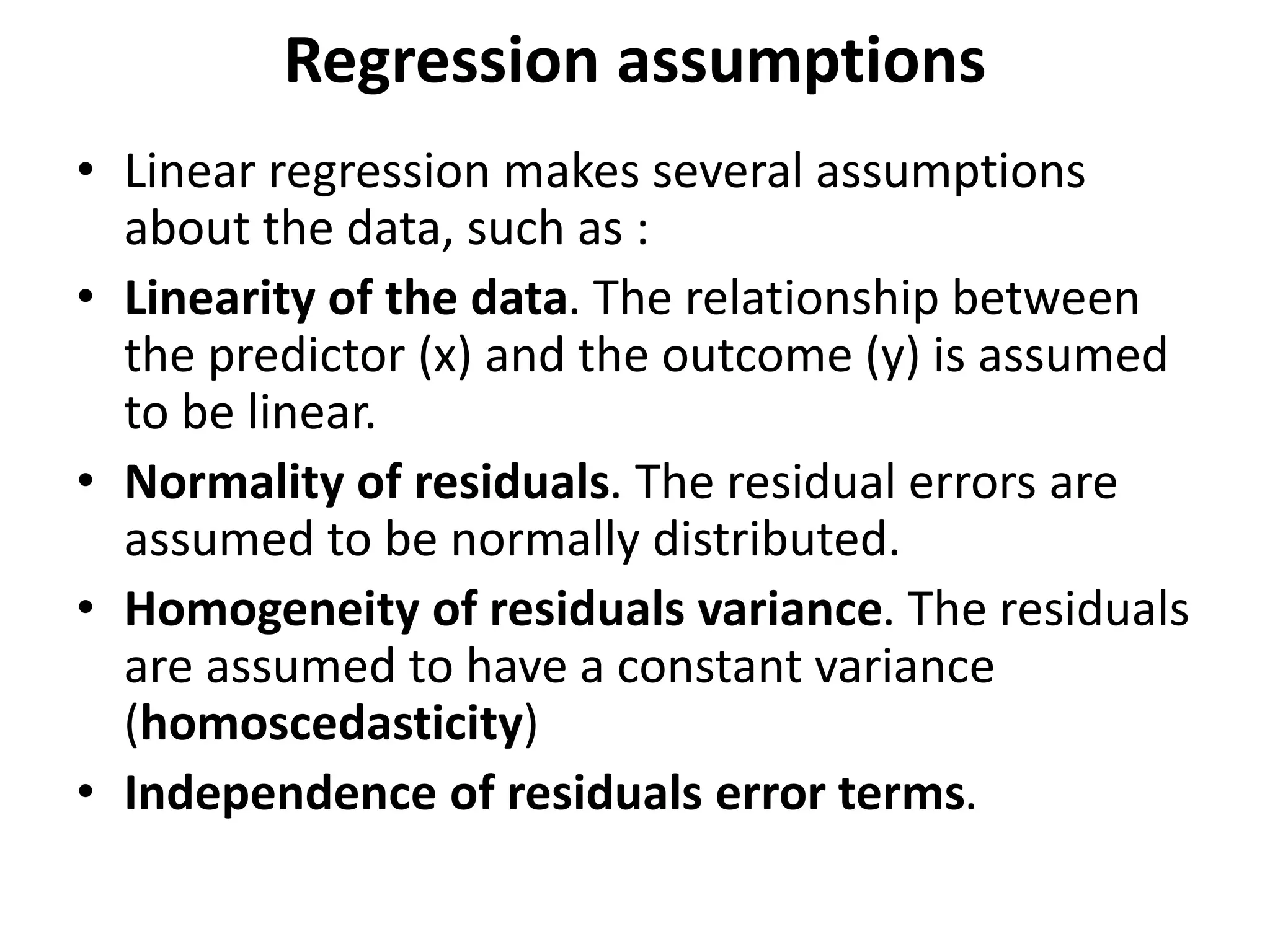
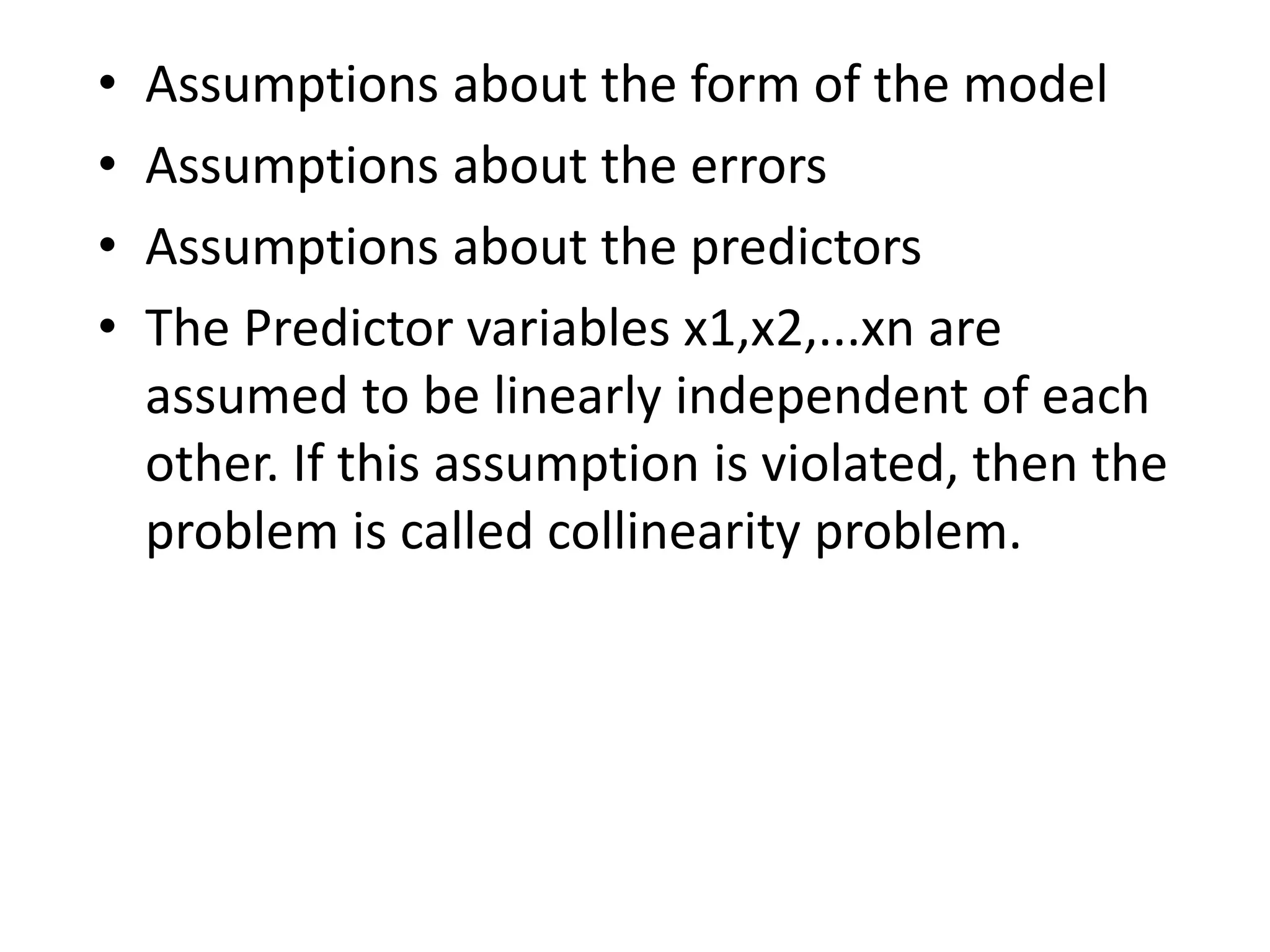
Discussion of linear regression assumptions including linearity, homoscedasticity, and normality of residuals.
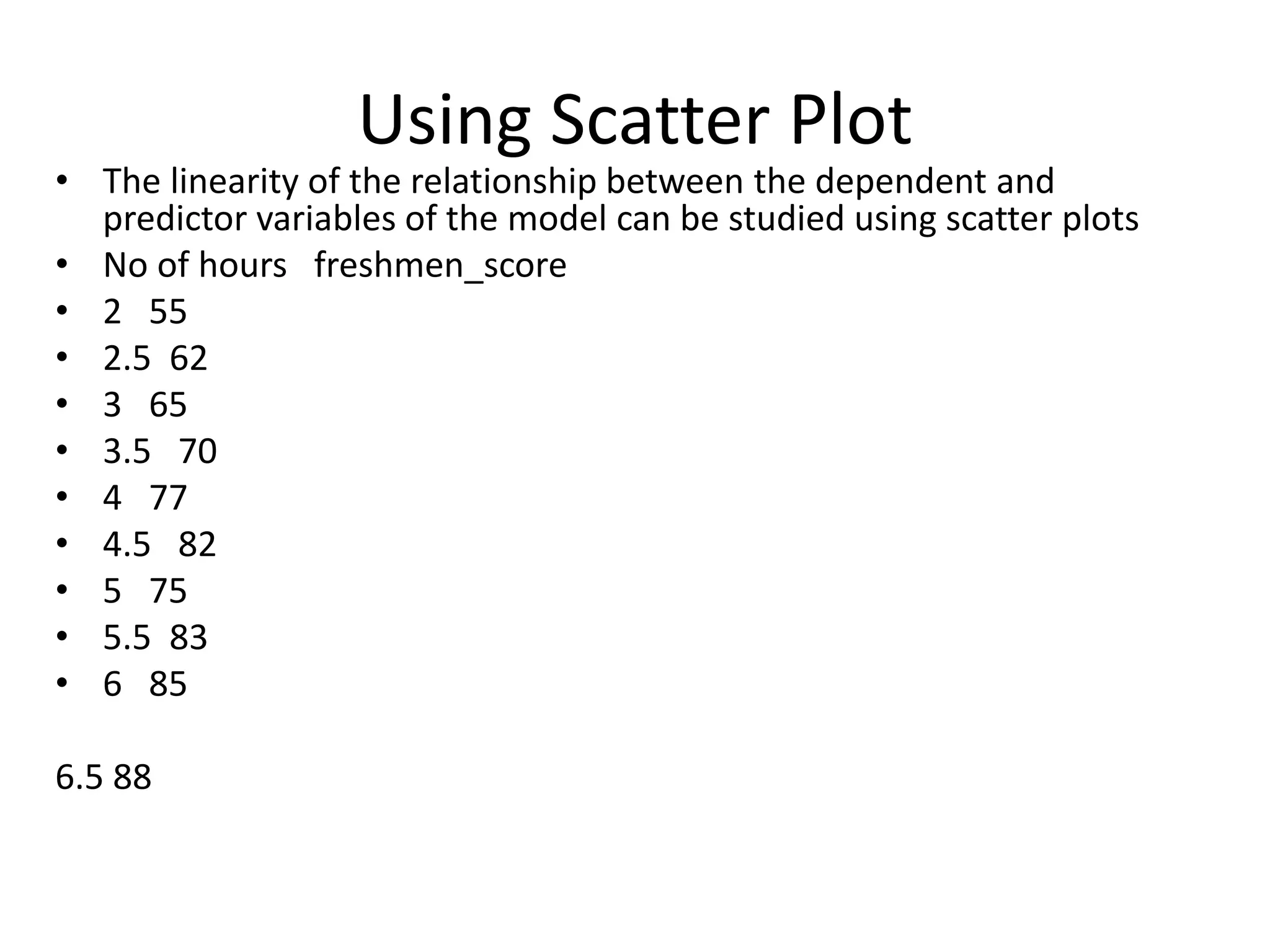
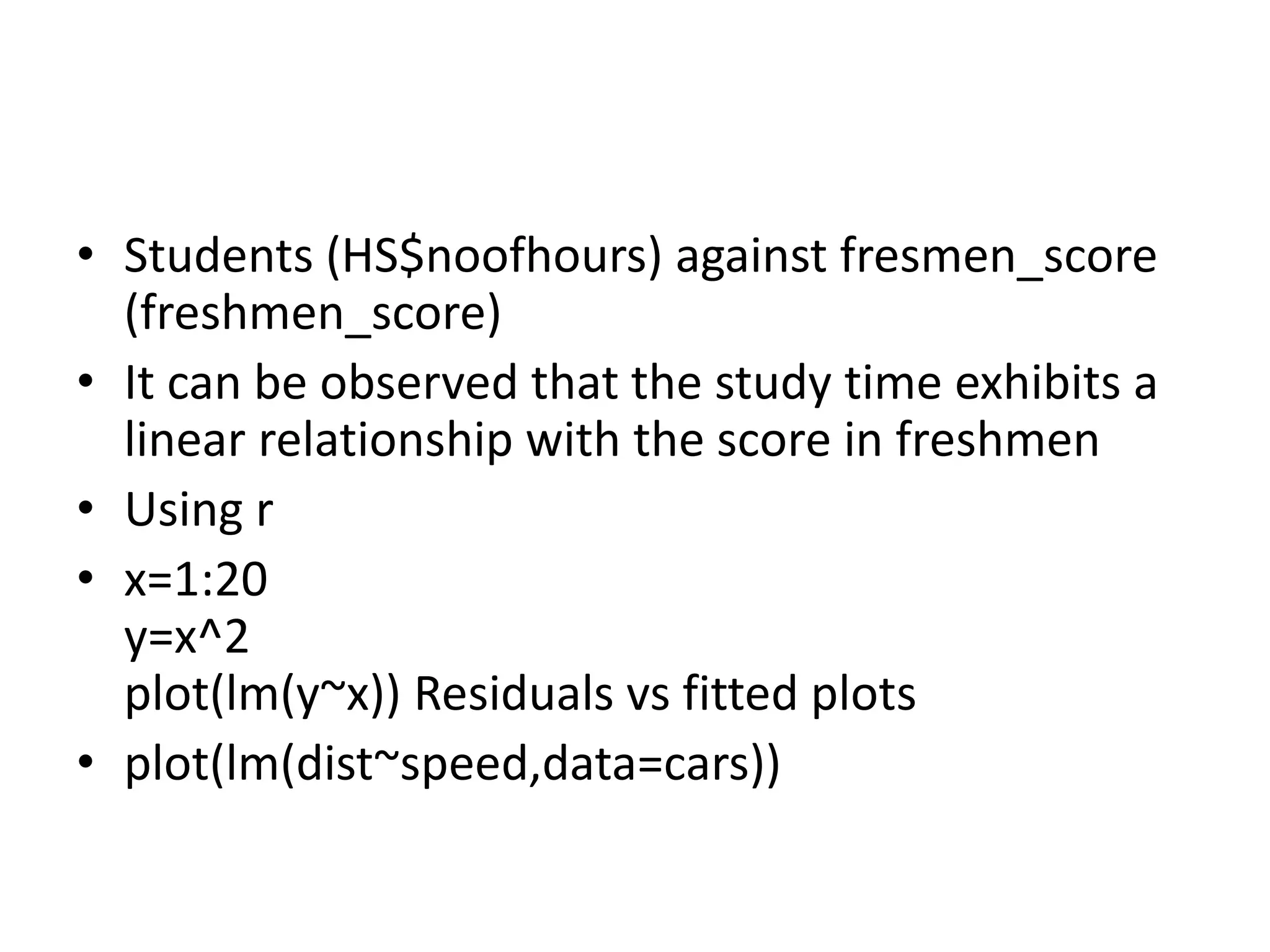
Examining the linear relationship through scatter plots and observing linearity in study time versus scores.
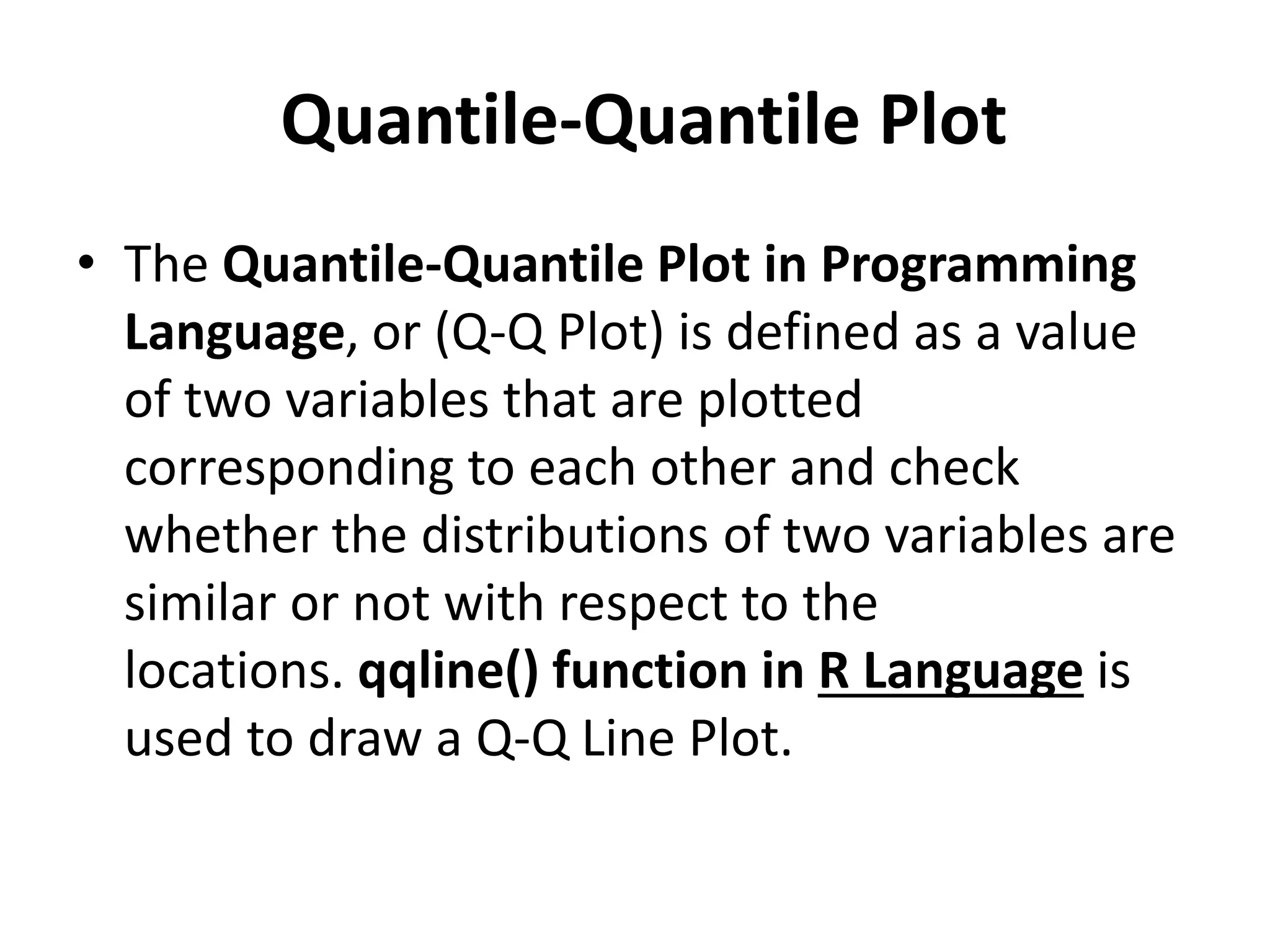
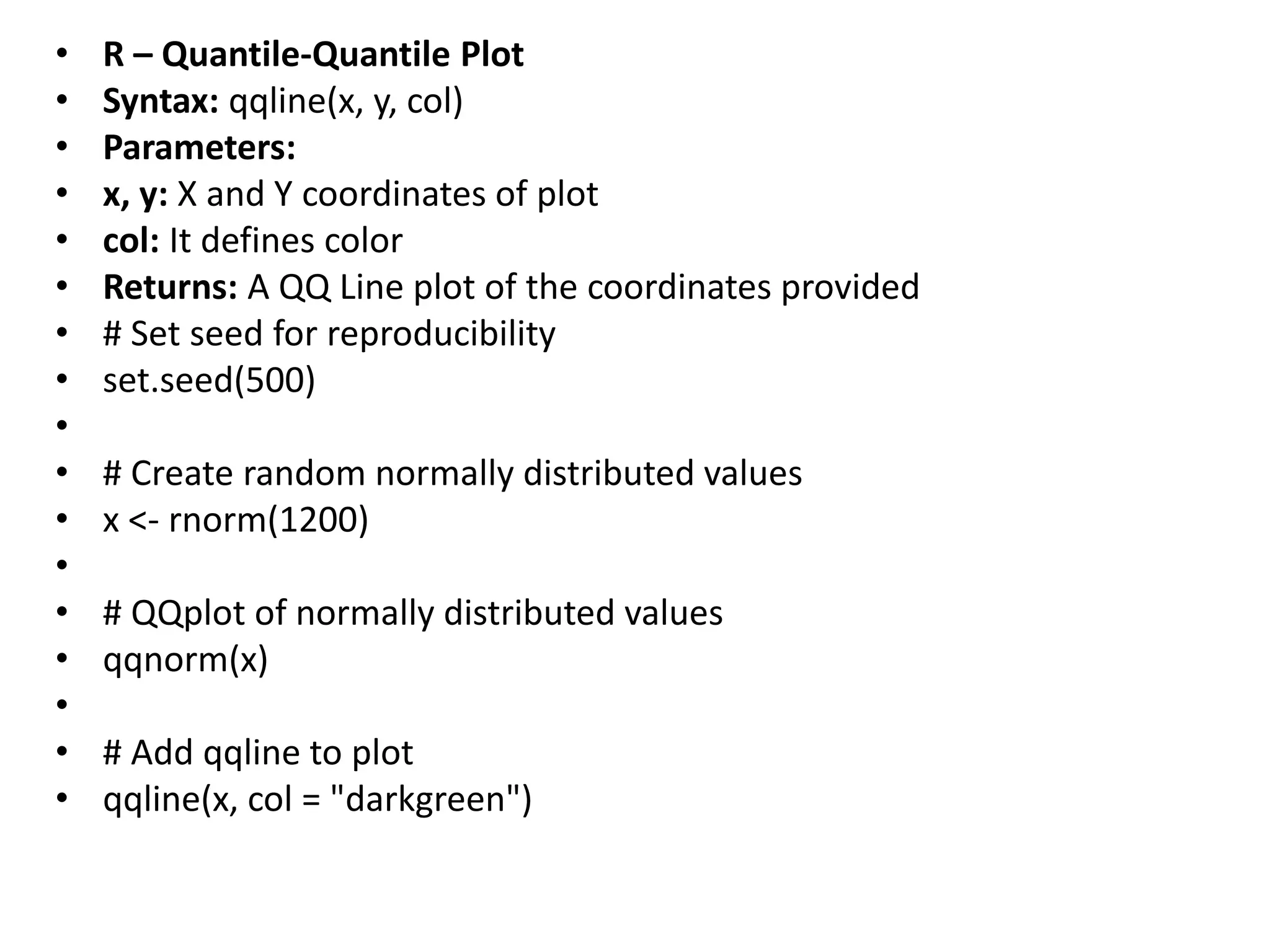
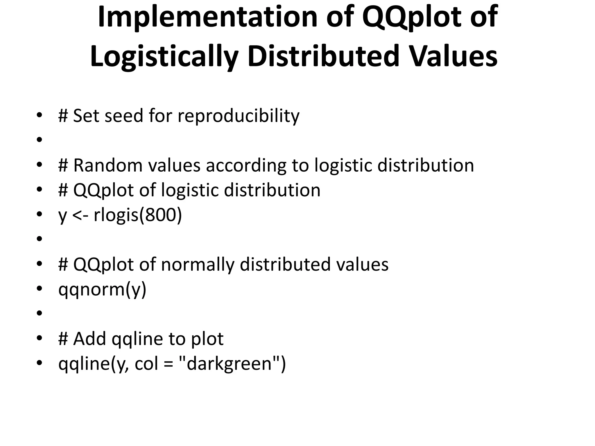
Explains QQ plots in R to compare data distributions and assess normality and logistic distribution.
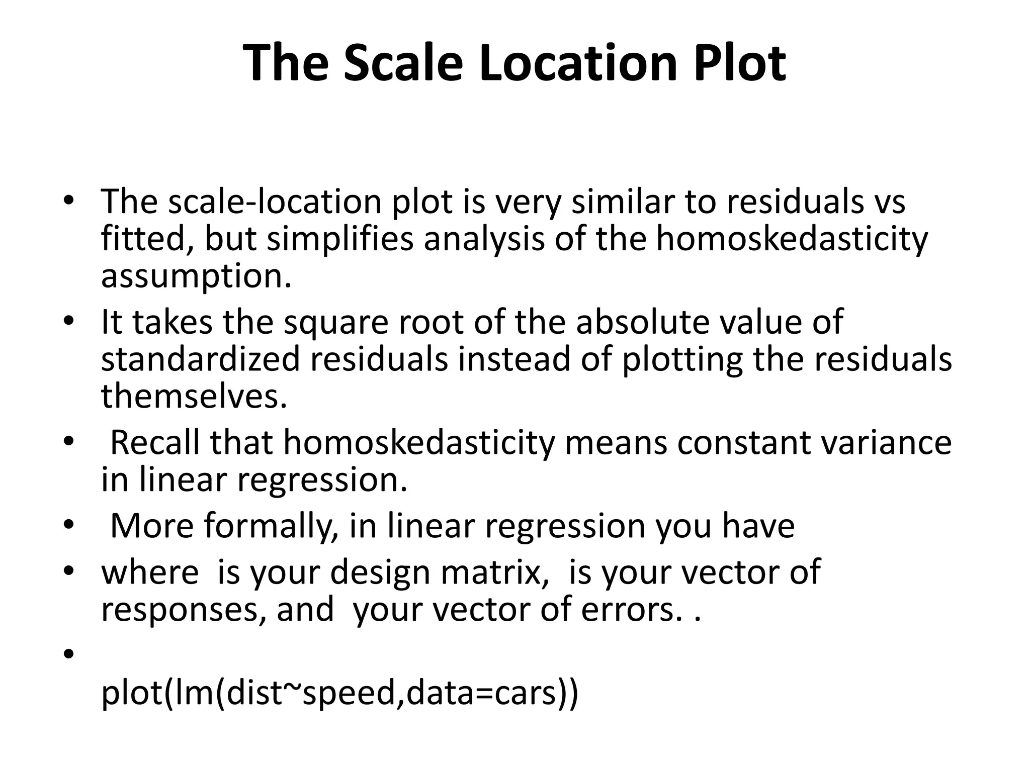
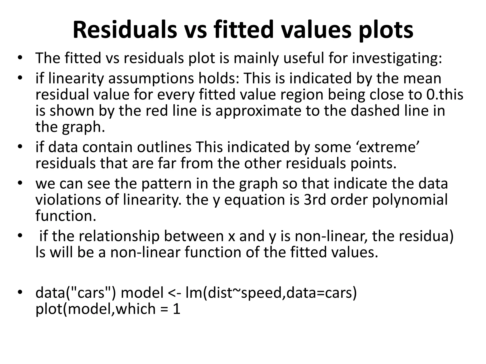
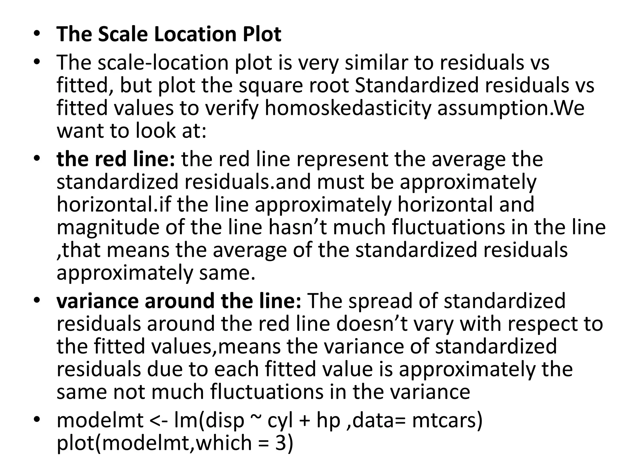
Utilizes Scale Location Plots and Residuals vs. Fitted Plots to check homoskedasticity and linearity assumptions.