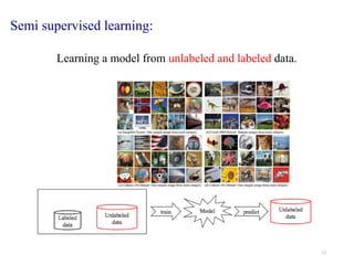
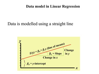
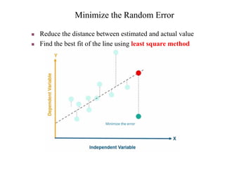
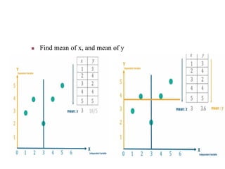
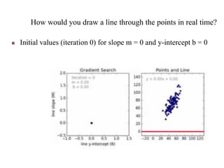
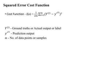
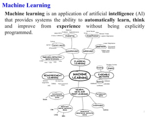
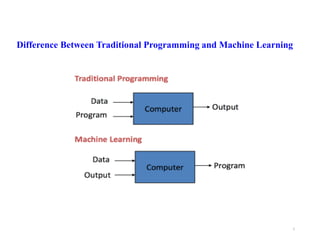
Machine learning is a form of artificial intelligence that allows systems to learn from data and improve automatically without being explicitly programmed. It works by building mathematical models based on sample data, known as "training data", in order to make predictions or decisions without being explicitly programmed to perform the task. Linear regression is a commonly used machine learning algorithm that allows predicting a dependent variable from an independent variable by finding the best fit line through the data points. It works by minimizing the sum of squared differences between the actual and predicted values of the dependent variable. Gradient descent is an optimization algorithm used to train machine learning models by minimizing a cost function relating predictions to ground truths.

1. Machine Learning
Dr. P. Kuppusamy
Prof / CSE

2. 2
Machine Learning
Machine learning is an application of artificial intelligence (AI)
that provides systems the ability to automatically learn, think
and improve from experience without being explicitly
programmed.

3. 3
Difference Between Traditional Programming and Machine Learning

4. Build a ML Model
4

5. ML Software Development
5
automatically learn and improve from experience

6. Features (Variables/Attributes) in ML
• Feature is an individual measurable attribute or characteristic of a
phenomenon being observed.
• Choosing informative, discriminating and independent features is
a crucial for effective algorithms in pattern
recognition, classification and regression.
• Features are usually numeric, but structural features such
as strings and graphs are used in syntactic pattern recognition.
• Eg. Table – Length, Breadth, Height, Weight, Color, Location,
no_of_draws, no_of _doors, Price

7. Features (Variables/Attributes) in ML
• Vector - collection / array of numbers in similar data type
• Feature Vector is an n-dimensional vector of
numerical features that represent some object.
• Eg. Length of 3 tables in feet
𝐿[1]
𝐿[2]
𝐿[3]
=
5
7
3

8. Feature extraction - definition
• Given a set of features 𝐹 = {𝑥1, … , 𝑥𝑁}
the Feature Extraction(“Construction”) problem is to map 𝐹 to
some feature set 𝐹′′ that maximizes the learner’s ability to
classify patterns

9. Feature Extraction
• Find a projection matrix w from n-dimensional to m-dimensional
vectors that keeps error low
𝒛 = 𝑤𝑇𝑿
w – Parameters
X – Set of features

10. Types of Learning
• Supervised (inductive) learning
• Training data includes desired outputs
• Unsupervised learning
• Training data does not include desired outputs
• Semi-supervised learning
• Training data includes a few desired outputs
• Reinforcement learning
• Rewards from sequence of actions

11. Supervised (Inductive) Learning
• Training data includes desired outputs
• Given examples of a function (X, F(X))
• Predict function F(X) for new examples X
• Discrete data - F(X): Classification
• Continuous data - F(X): Regression
• F(X) = Probability(X): Probability estimation

12. 12
Supervised learning:
Learning a model from labeled data.

13. 13
Supervised learning
Algorithms: Regression, Support Vector Machines, neural
networks, decision trees, K-nearest neighbors, naive Bayes, etc.

14. 14
Unsupervised learning
Algorithms: K-means, gaussian mixtures, hierarchical clustering,
spectral clustering, etc.
Learning a model from unlabeled data.

15. 15
Semi supervised learning:
Learning a model from unlabeled and labeled data.

16. Linear Regression
• Linear Regression analysis is a statistical tool
• Predictive modeling method to investigate the mathematical
relationship between a dependent variable (outcome – y) and an
independent variable (predictor – x).
• Predictor shows the changes in Dependent variable (y axis) to the
changes in explanatory variables in X axis.

17. Linear Regression
• It is quantitative analysis tool
• It uses current information about a phenomenon to predict its future behavior.
• Involves the graphical lines over a set of data points that most closely towards
all shape of the data.
• when the data form a set of pairs of numbers, it is interpreted as the observed
values of an independent (or predictor ) variable X and a dependent ( or
response) variable Y.

18. y x
  
  
0 1
Data model in Linear Regression
• Data is modelled using a straight line with continuous variable
• Relationship between variables is a linear function
Dependent
(Response)
Variable
Independent
(Explanatory)
Variable
Population
Slope
Population
y-intercept
Random
Error

19. y
β0 = y-intercept
x
Change
in y
Change in x
β1 = Slope
Data model in Linear Regression
Data is modelled using a straight line

20. Types of Relationships
Y
X
Y
X
Y
Y
X
X
Strong relationships Weak relationships

21. Types of Relationships
Y
X
Y
X
No relationship
(continued)

22. Plot for x and actual y values
 Plot the graph using x and y values

23. Random Error Identification
 Random Error  = Estimated Value (yi) – Actual Value (yi)

24. Minimize the Random Error
 Reduce the distance between estimated and actual value
 Find the best fit of the line using least square method

25. Least Squares Method to Minimize the Error
• ‘Best fit’ means difference between actual y values and
predicted y values are a minimum
• But positive differences off-set negative
 
2 2
1 1
ˆ ˆ
n n
i
i i
i i
y y 
 
 
 
• Least Squares minimizes the Sum of the Squared Differences
(SSE)

26. Least Squares Graphically
2
y
x
1 3
4
^
^
^
^
2 0 1 2 2
ˆ ˆ ˆ
y x
  
  
0 1
ˆ ˆ
ˆi i
y x
 
 
2 2 2 2 2
1 2 3 4
1
ˆ ˆ ˆ ˆ ˆ
LS minimizes
n
i
i
    

   


27. Case Study
 Let consider x and y values and mark in scatter plot

28.  Find mean of x, and mean of y

29.  Find the coefficients m and c in the straight line y = mx+c

30.  Find x-x1, and y-y1

31.  Find m

32. Plot the x, y values in the graph
x = {1, 2, 3, 4, 5} y = {3, 4, 2, 4, 5}

33. Plot the regression line using estimated y values
x = {1, 2, 3, 4, 5} y = {2.8, 3.2, 3.6, 4, 4.4}
Estimated y values
Estimated y values

34. Find the Error 
Mean Square Error minimizes the
error in the linear regression.
Regression Line with least error is
the ‘best fit’ line
 
2 2
1 1
ˆ ˆ
n n
i
i i
i i
y y 
 
 
 

35. How would you draw a line through the points in real time?
 Initial values (iteration 0) for slope m = 0 and y-intercept b = 0

36. How would you draw a line through the points?
iteration 1, slope m = 0.04 and y-
intercept b = 0
iteration 20, slope m = 0.59 and y-
intercept b = 0.01

37. Determine which line ‘fits best’ in 100 iterations
iteration 47, slope m = 1.03 and y-
intercept b = 0.02
iteration 99, slope m = 1.36 and y-
intercept b = 0.03

38. 3 major Uses of Regression
•Determining the strength of predictors
•Forecasting an effect
•Trend forecasting

39. Where Linear Regression used?
• Evaluating trends and sales estimates
• Analyze the impact of price changes
• Insurance domain

40. Squared Error Cost Function
• Cost Function - J(ɵ) =
1
2𝑚
σ𝑖=1
𝑚
(𝑌(𝑖)
− 𝑦′ 𝑖
)2
𝑌(𝑖) - Ground truths or Actual output or label
𝑦′ 𝑖
- Prediction output
m - No. of data points or samples

41. Gradient Descent
• The objective of training a machine learning model is to minimize the loss or error
between ground truths and predictions by changing the trainable parameters.
• Gradient is the extension of derivative in multi-dimensional space, tells the direction
along which the loss or error is optimally minimized.
• Gradient is defined as the maximum rate of change.
𝜃𝑗 = 𝜃𝑗 − 𝛼
𝜕
𝜕𝜃𝑗
𝐽(𝜃)
• 𝜃𝑗-Training parameter 𝛼 – Learning rate 𝐽(𝜃) – Error / Cost function

42. Gradient Descent
• Gradient Descent:
𝜃𝑗 = 𝜃𝑗 − 𝛼
1
𝑚
σ𝑖=1
𝑚
(𝑦′(𝑖)
−𝑌 𝑖 )𝑥𝑗
𝑖
for All j
j=0; 𝜃0 = 𝜃0 − 𝛼
1
𝑚
σ𝑖=1
𝑚
(𝑦′(𝑖)
−𝑌 𝑖 )𝑥0
𝑖
for All j
j=1; 𝜃1 = 𝜃1 − 𝛼
1
𝑚
σ𝑖=1
𝑚
(𝑦′(𝑖)
−𝑌 𝑖 )𝑥1
𝑖
for All j
………..
j=n; 𝜃𝑛 = 𝜃𝑛 − 𝛼
1
𝑚
σ𝑖=1
𝑚
(𝑦′(𝑖)
−𝑌 𝑖 )𝑥𝑛
𝑖 for All j

43. References
• Tom Markiewicz& Josh Zheng,Getting started with Artificial
Intelligence, Published by O’Reilly Media,2017
• Stuart J. Russell and Peter Norvig,Artificial Intelligence A Modern
Approach
• Richard Szeliski, Computer Vision: Algorithms and Applications,
Springer 2010
• Artificial Intelligence and Machine Learning, Chandra S.S. & H.S.
Anand, PHI Publications
• Machine Learning, Rajiv Chopra, Khanna Publishing House
•