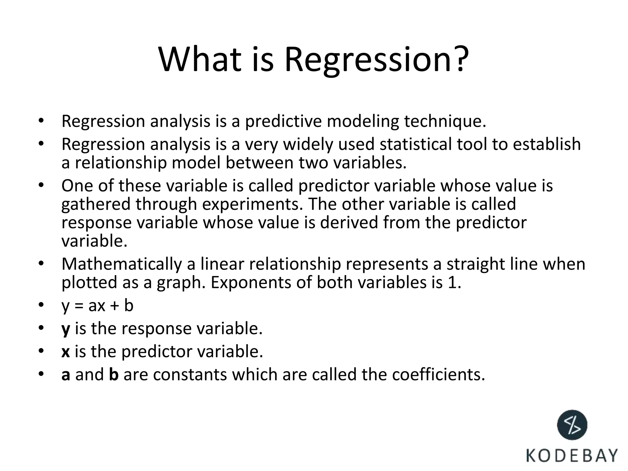
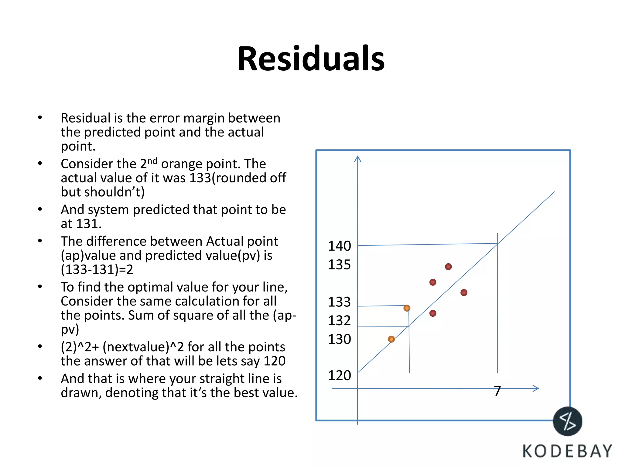
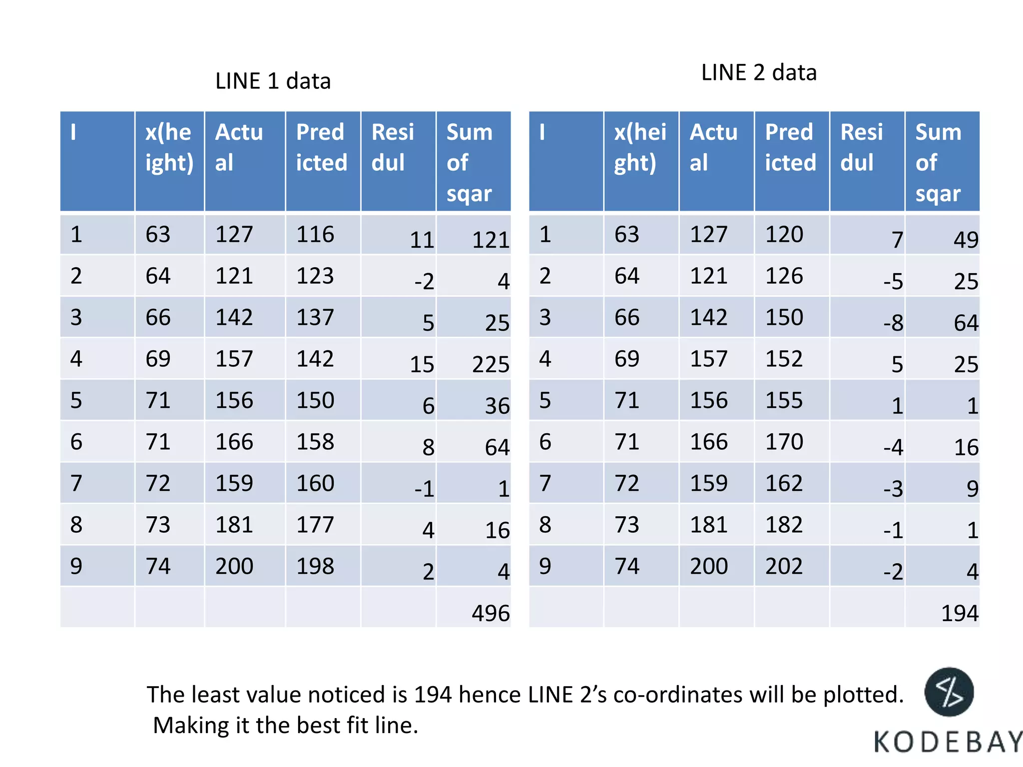
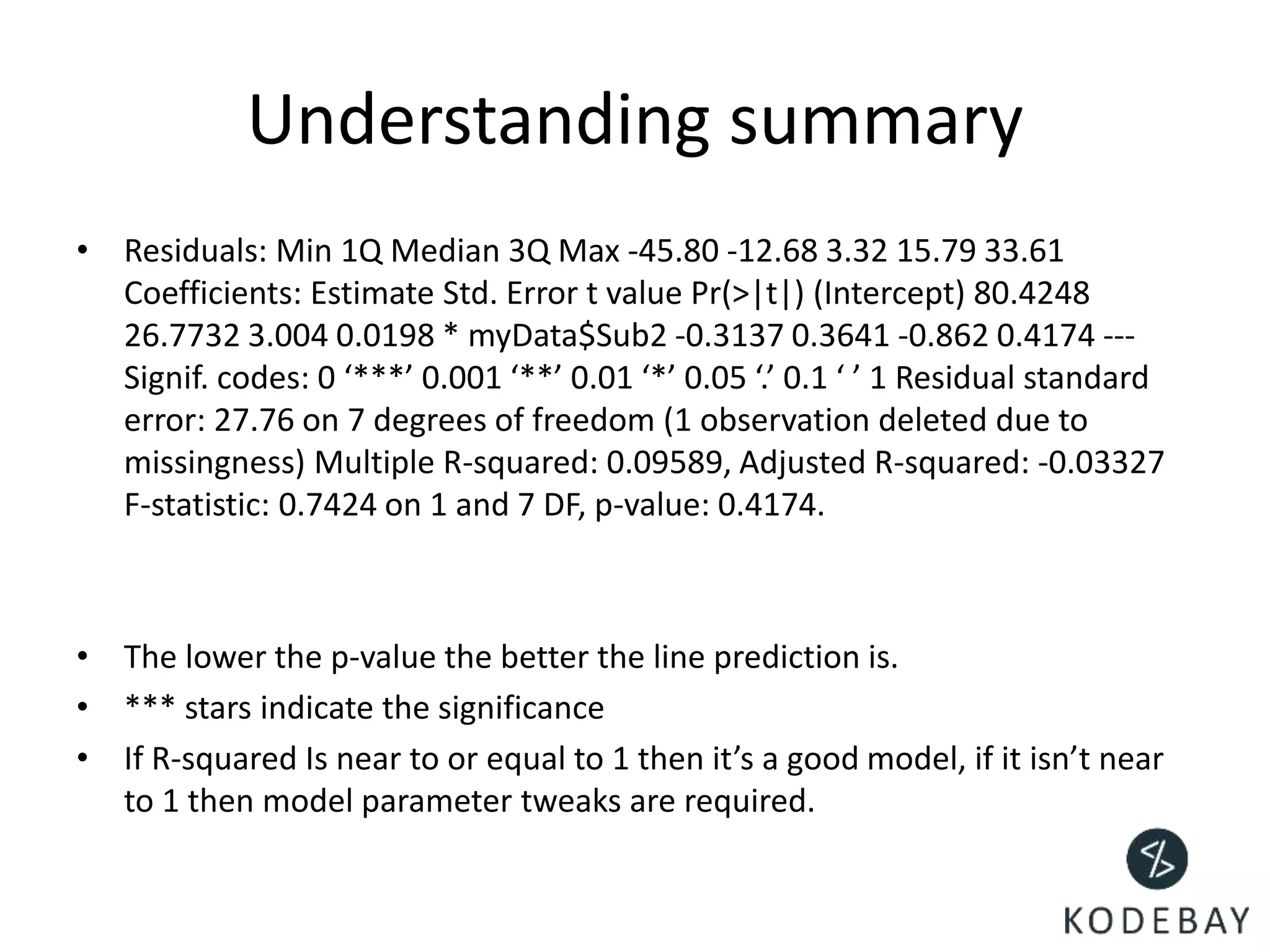
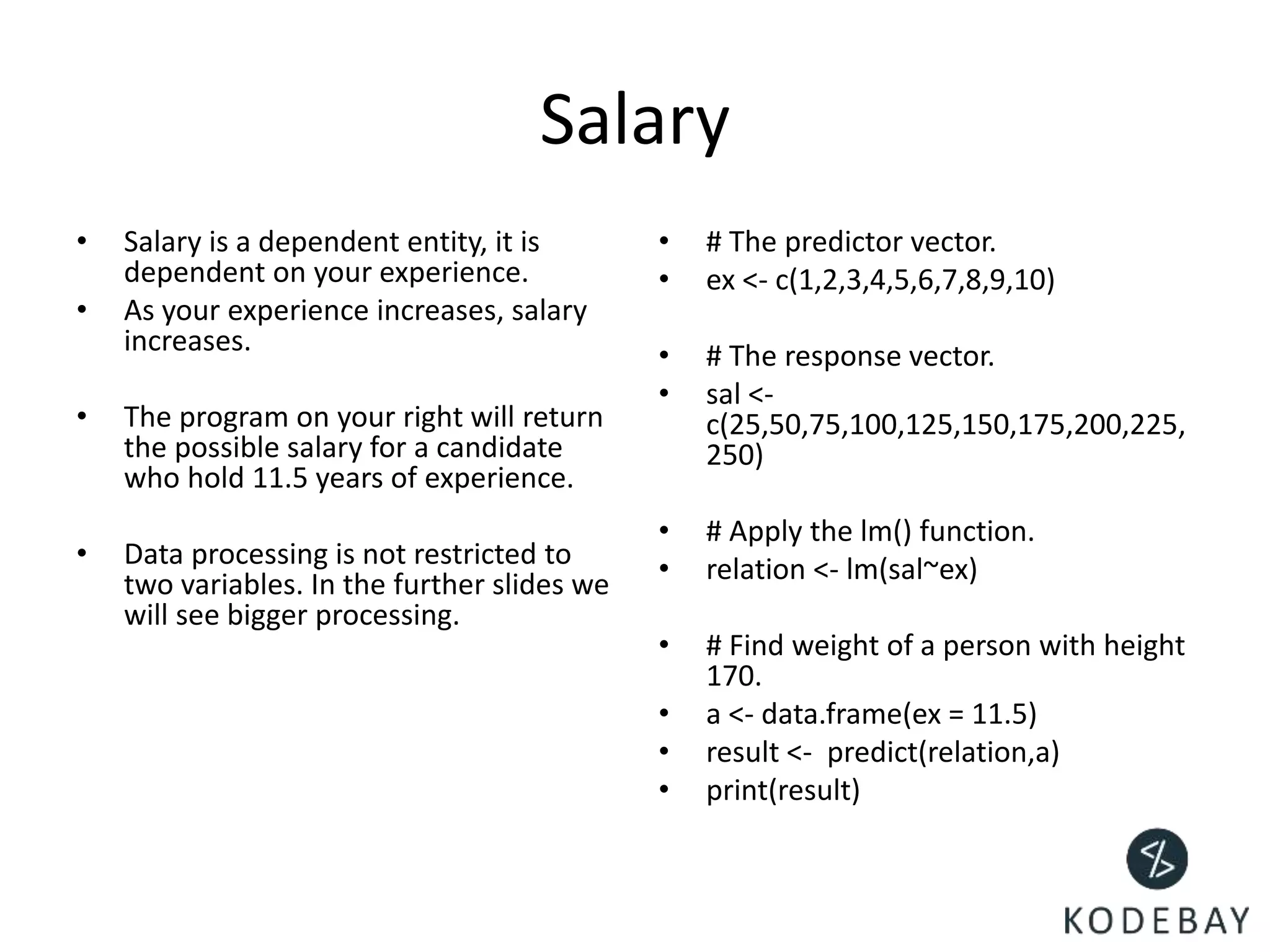
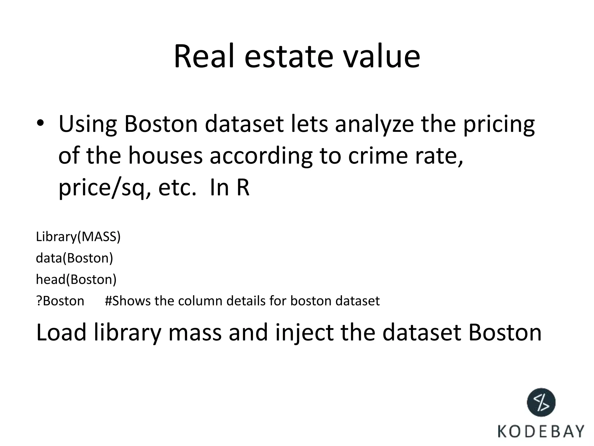
- Linear regression is a predictive modeling technique used to establish a relationship between two variables, known as the predictor and response variables. - The residuals are the errors between predicted and actual values, and the optimal regression line is the one that minimizes the sum of squared residuals. - Linear regression can be used to predict variables like salary based on experience, or housing prices based on features like crime rates or school quality. Co-relation analysis examines the relationships between predictor variables.

1. Linear Regression

2. What is Regression?
• Regression analysis is a predictive modeling technique.
• Regression analysis is a very widely used statistical tool to establish
a relationship model between two variables.
• One of these variable is called predictor variable whose value is
gathered through experiments. The other variable is called
response variable whose value is derived from the predictor
variable.
• Mathematically a linear relationship represents a straight line when
plotted as a graph. Exponents of both variables is 1.
• y = ax + b
• y is the response variable.
• x is the predictor variable.
• a and b are constants which are called the coefficients.

3. Residuals
• Residual is the error margin between
the predicted point and the actual
point.
• Consider the 2nd orange point. The
actual value of it was 133(rounded off
but shouldn’t)
• And system predicted that point to be
at 131.
• The difference between Actual point
(ap)value and predicted value(pv) is
(133-131)=2
• To find the optimal value for your line,
Consider the same calculation for all
the points. Sum of square of all the (ap-
pv)
• (2)^2+ (nextvalue)^2 for all the points
the answer of that will be lets say 120
• And that is where your straight line is
drawn, denoting that it’s the best value. 7
140
135
133
132
130
120

4. WHERE CAN YOU USE THIS?
(SAMPLE ATTACHED IN NEXT SLIDE)

5. LETS TAKE AN EXAMPLE OF HEIGHT
AND WEIGHT

6. Lets use a dataset of 10 students height and
weight to draw scatterplot(graph)
Height Weight
63 127
64 121
66 142
69 157
71 156
71 166
72 159
73 181
74 200
0
50
100
150
200
250
60 70 80
Y-Values
Y-Values

7. The questions is what is the best fitting line
if plotted for the chart
• Residual error is calculated by
Err=actual value-predicted value
• Using sum of squared technique we find the total of
all the squared values.
• The answer which is the lowest is selected as the
best fit line.
• Consider the next slide for more example

8. I x(he
ight)
Actu
al
Pred
icted
Resi
dul
Sum
of
sqar
1 63 127 116 11 121
2 64 121 123 -2 4
3 66 142 137 5 25
4 69 157 142 15 225
5 71 156 150 6 36
6 71 166 158 8 64
7 72 159 160 -1 1
8 73 181 177 4 16
9 74 200 198 2 4
496
I x(hei
ght)
Actu
al
Pred
icted
Resi
dul
Sum
of
sqar
1 63 127 120 7 49
2 64 121 126 -5 25
3 66 142 150 -8 64
4 69 157 152 5 25
5 71 156 155 1 1
6 71 166 170 -4 16
7 72 159 162 -3 9
8 73 181 182 -1 1
9 74 200 202 -2 4
194
LINE 1 data LINE 2 data
The least value noticed is 194 hence LINE 2’s co-ordinates will be plotted.
Making it the best fit line.

9. Salary
• Salary is a dependent entity, it is
dependent on your experience.
• As your experience increases, salary
increases.
• The program on your right will return
the possible salary for a candidate
who hold 11.5 years of experience.
• Data processing is not restricted to
two variables. In the further slides we
will see bigger processing.
• # The predictor vector.
• ex <- c(1,2,3,4,5,6,7,8,9,10)
• # The response vector.
• sal <-
c(25,50,75,100,125,150,175,200,225,
250)
• # Apply the lm() function.
• relation <- lm(sal~ex)
• # Find weight of a person with height
170.
• a <- data.frame(ex = 11.5)
• result <- predict(relation,a)
• print(result)

10. Real estate value
• Using Boston dataset lets analyze the pricing
of the houses according to crime rate,
price/sq, etc. In R
Library(MASS)
data(Boston)
head(Boston)
?Boston #Shows the column details for boston dataset
Load library mass and inject the dataset Boston

11. • Lets separate the dataset so that we can process
values and compare the prediction results to the
actual values. Let it be a 70-30 split.
set.seed(2)
library(caTools) #install package caTools
split<-sample.split(Boston$medv,SplitRatio = 0.7)
split
training_dataset<-subset(Boston,split==TRUE)
testing_dataset<-subset(Boston,split==FALSE)
Here the split is 70-30, 70 to train the model and 30
to see whether the predictions are correct
comparing it to the data we already have.

12. Co-relations
• Co-relations is an important factor to check the
dependencies within themselves and on other
vars.
• Co-relation gives us an insight to find the
relationship shared by two sets.
• cr<- cor(Boston)
will return the co-relation b/w elements belonging
to the dataset of Boston
library(corrplot)
corrplot(cr,type=“lower”)

13. Multi-Colinearity
• When there is a high co-relation of one
element with another we can say that the
elements are related, in order to know
multicollinearity we use vif().
• Not important for this dataset

14. Understanding summary
• Residuals: Min 1Q Median 3Q Max -45.80 -12.68 3.32 15.79 33.61
Coefficients: Estimate Std. Error t value Pr(>|t|) (Intercept) 80.4248
26.7732 3.004 0.0198 * myData$Sub2 -0.3137 0.3641 -0.862 0.4174 ---
Signif. codes: 0 ‘***’ 0.001 ‘**’ 0.01 ‘*’ 0.05 ‘.’ 0.1 ‘ ’ 1 Residual standard
error: 27.76 on 7 degrees of freedom (1 observation deleted due to
missingness) Multiple R-squared: 0.09589, Adjusted R-squared: -0.03327
F-statistic: 0.7424 on 1 and 7 DF, p-value: 0.4174.
• The lower the p-value the better the line prediction is.
• *** stars indicate the significance
• If R-squared Is near to or equal to 1 then it’s a good model, if it isn’t near
to 1 then model parameter tweaks are required.

15. lm()
• Model building is done by lm() function.
Model<-lm(value_of_home,
area+crimerate+age…,data=training_data)
• If the summary of model returns elements
which do not have more than *(1 star) it is
advisable to remove the parameter from the
lm()

16. Model
• A model is developed so that its precision to
predict future data is high. If the R-squared
value is low then the model is not good. If the
p-value is near 0 then it’s a good model.
model <-lm(Boston$medv~ Boston$crim+Boston$zn+Boston$indus+Boston$chas,Boston$nos,Boston$rm)
summary(model)
The first parameter is what the data is plotted against.

17. SUPPORT@KODEBAY.COM
Email for support