Download to read offline
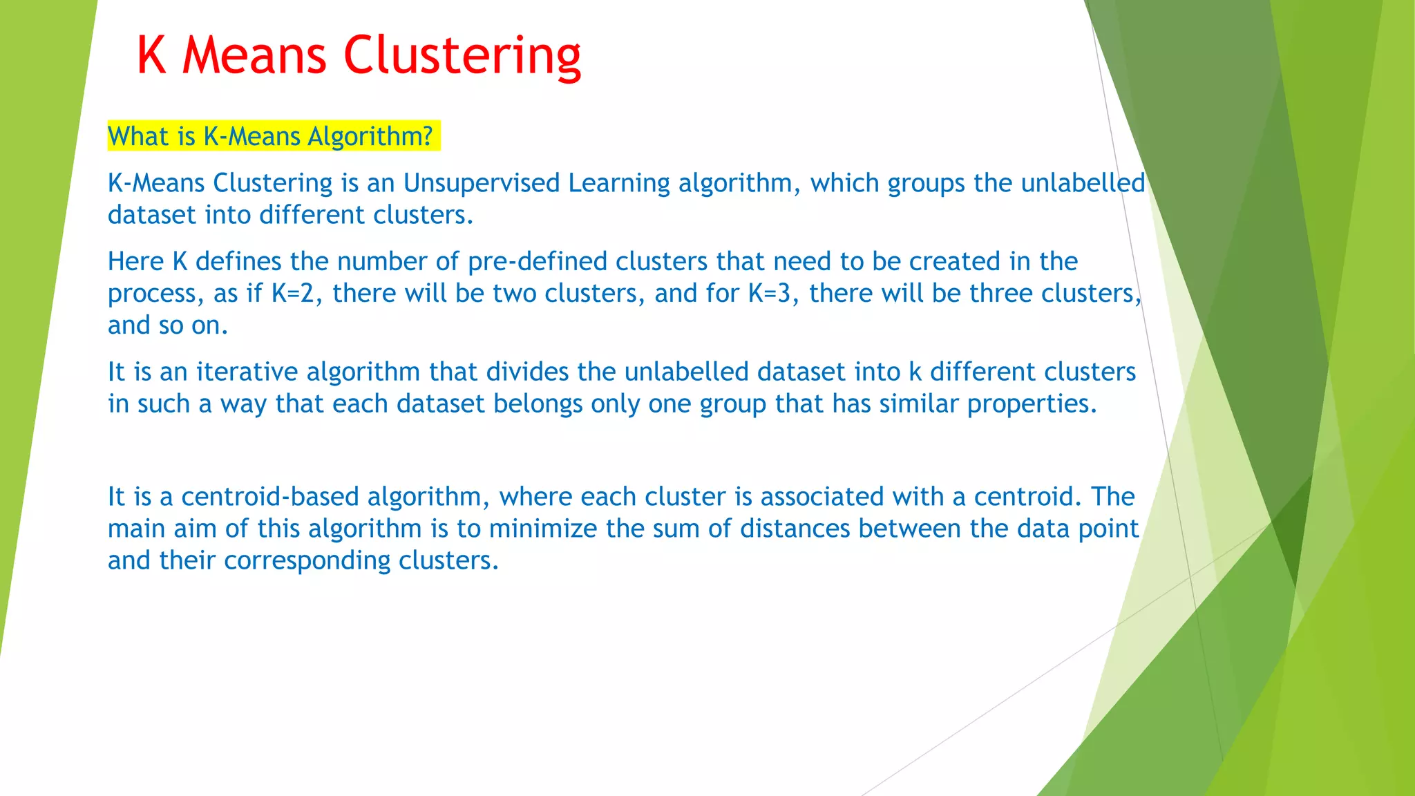


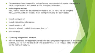

![ #finding optimal number of clusters using the elbow method
from sklearn.cluster import KMeans
wcss_list= [] #Initializing the list for the values of WCSS
#Using for loop for iterations from 1 to 10.
for i in range(1, 11):
kmeans = KMeans(n_clusters=i, init='k-means++', random_state= 42)
kmeans.fit(x)
wcss_list.append(kmeans.inertia_)
mtp.plot(range(1, 11), wcss_list)
mtp.title('The Elobw Method Graph')
mtp.xlabel('Number of clusters(k)')
mtp.ylabel('wcss_list')
mtp.show()](https://image.slidesharecdn.com/kmeansclusteringinml-230914052929-d0d23d39/85/K-Means-Clustering-in-ML-pptx-9-320.jpg)

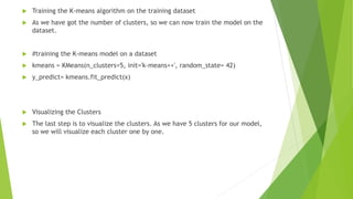
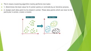
![ #visulaizing the clusters
mtp.scatter(x[y_predict == 0, 0], x[y_predict == 0, 1], s = 100, c = 'blue', label = 'Cluster 1') #for first cluster
mtp.scatter(x[y_predict == 1, 0], x[y_predict == 1, 1], s = 100, c = 'green', label = 'Cluster 2') #for second cluster
mtp.scatter(x[y_predict== 2, 0], x[y_predict == 2, 1], s = 100, c = 'red', label = 'Cluster 3') #for third cluster
mtp.scatter(x[y_predict == 3, 0], x[y_predict == 3, 1], s = 100, c = 'cyan', label = 'Cluster 4') #for fourth cluster
mtp.scatter(x[y_predict == 4, 0], x[y_predict == 4, 1], s = 100, c = 'magenta', label = 'Cluster 5') #for fifth cluster
mtp.scatter(kmeans.cluster_centers_[:, 0], kmeans.cluster_centers_[:, 1], s = 300, c = 'yellow', label = 'Centroid'
)
mtp.title('Clusters of customers')
mtp.xlabel('Annual Income (k$)')
mtp.ylabel('Spending Score (1-100)')
mtp.legend()
mtp.show()](https://image.slidesharecdn.com/kmeansclusteringinml-230914052929-d0d23d39/85/K-Means-Clustering-in-ML-pptx-12-320.jpg)

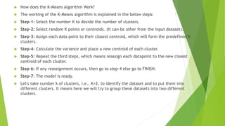
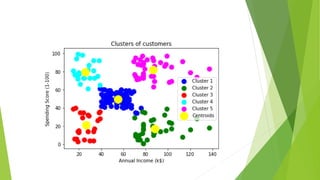
![ import numpy as nm
import matplotlib.pyplot as mtp
import pandas as pd
dataset = pd.read_csv('Mall_Customers_data.csv')
print(dataset)
x = dataset.iloc[:, [3, 4]].values
print(x)
#finding optimal number of clusters using the elbow method
from sklearn.cluster import KMeans
wcss_list=[]
#Initializing the list for the values of WCSS
#Using for loop for iterations from 1 to 10.
for i in range(1,11):
kmeans=KMeans(n_clusters=i,init='k-means++',random_state=42)
kmeans.fit(x)
wcss_list.append(kmeans.inertia_)
mtp.plot(range(1,11),wcss_list)
mtp.title('The Elobw Method Graph')](https://image.slidesharecdn.com/kmeansclusteringinml-230914052929-d0d23d39/85/K-Means-Clustering-in-ML-pptx-14-320.jpg)
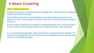
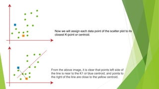
![ mtp.xlabel('Number of clusters(k)')
mtp.ylabel('wcss_list')
mtp.show()
#training the K-means model on a dataset
kmeans = KMeans(n_clusters=5, init='k-means++', random_state= 42)
y_predict= kmeans.fit_predict(x)
#visulaizing the clusters
mtp.scatter(x[y_predict == 0, 0], x[y_predict == 0, 1], s = 100, c = 'blue', label = 'Cluster 1') #for first cluster
mtp.scatter(x[y_predict == 1, 0], x[y_predict == 1, 1], s = 100, c = 'green', label = 'Cluster 2') #for second cluster
mtp.scatter(x[y_predict== 2, 0], x[y_predict == 2, 1], s = 100, c = 'red', label = 'Cluster 3') #for third cluster
mtp.scatter(x[y_predict == 3, 0], x[y_predict == 3, 1], s = 100, c = 'cyan', label = 'Cluster 4') #for fourth cluster
mtp.scatter(x[y_predict == 4, 0], x[y_predict == 4, 1], s = 100, c = 'magenta', label = 'Cluster 5') #for fifth cluster
mtp.scatter(kmeans.cluster_centers_[:, 0], kmeans.cluster_centers_[:, 1], s = 300, c = 'yellow', label =
'Centroid')
mtp.title('Clusters of customers')
mtp.xlabel('Annual Income (k$)')
mtp.ylabel('Spending Score (1-100)')
mtp.legend()
mtp.show()](https://image.slidesharecdn.com/kmeansclusteringinml-230914052929-d0d23d39/85/K-Means-Clustering-in-ML-pptx-15-320.jpg)

K-Means clustering is an unsupervised learning algorithm that groups unlabeled data points into K number of clusters based on their similarity. It works by first randomly selecting K cluster centers, known as centroids. It then assigns each data point to the closest centroid, forming K clusters. It then recalculates the position of the centroids and reassigns data points in an iterative process, until the centroids are stable or the maximum number of iterations is reached. The optimal number of clusters K is determined using the elbow method by plotting the within-cluster sum of squares (WCSS) against the number of clusters K.