The document discusses decision trees and their use in R. It contains 3 key points: 1. Decision trees can be used to predict outcomes like spam detection based on input variables. The nodes represent choices and edges represent decision rules. 2. An example creates a decision tree using the 'party' package in R to predict reading skills based on variables like age, shoe size, and native language. 3. The 'rpart' package can also be used to create and visualize decision trees, as shown through an example predicting insurance fraud based on rear-end collisions.

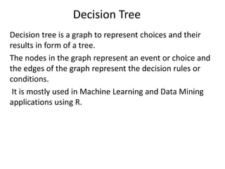
1. Decision Tree
Decision tree is a graph to represent choices and their
results in form of a tree.
The nodes in the graph represent an event or choice and
the edges of the graph represent the decision rules or
conditions.
It is mostly used in Machine Learning and Data Mining
applications using R.

2. Examples
• predicting an email as spam or not spam.
• predicting of a tumour is cancerous or not .
• predicting a loan as a good or bad credit risk based
on the factors in each of these.
• Generally, a model is created with observed data
also called training data.
• Then a set of validation data is used to verify and
improve the model.
• R has packages which are used to create and
visualize decision trees.
• For new set of predictor variable, we use this model
to arrive at a decision on the category (yes/No,
spam/not spam) of the data.

3. • The R package "party" is used to create decision
trees.
• Install R Package
• Use the below command in R console to install
the package. You also have to install the
dependent packages if any.
• install.packages("party")
• The package "party" has the function ctree()(is
used to create recursive tree), conditional
inference tree, which is used to create and
analyze decision tree.

4. • Syntax
• The basic syntax for creating a decision tree in R is −
• ctree(formula, data) Following is the description of
the parameters used −
• formula is a formula describing the predictor and
response variables.
• data is the name of the data set used.
Input Data
• We will use the R in-built data set
named readingSkills to create a decision tree.
• It describes the score of someone's readingSkills if
we know the variables "age","shoesize","score" and
whether the person is a native speaker or not.
• Here is the sample data.

5. • # Load the party package.
• It will automatically load other # dependent
packages.
• library(party) # Print some records from data
set readingSkills.
• print(head(readingSkills))
• Example
• We will use the ctree() function to create the
decision tree and see its graph.

6. • # Load the party package.
• It will automatically load other # dependent packages.
• library(party)
• # Create the input data frame.
• InputData <- readingSkills[c(1:105),]
• # Give the chart file a name. It is the name of the output
file
• png(file = "decision_tree.png")
• # Create the tree.
• outputTree <- ctree( nativeSpeaker ~ age + shoeSize +
score, data = InputData )
• # Plot the tree.
• plot(outputTree )
• # Save the file.
• dev.off()

7. • When we execute the above code, it produces the
following result −
• null device 1
• Loading required package: methods
• Loading required package: grid
• Loading required package: mvtnorm
• Loading required package: modeltools
• Loading required package: stats4
• Loading required package: strucchange
• Loading required package: zoo
• Attaching package: ‘zoo’
• The following objects are masked from
‘package:base’: as.Date, as.Date.numeric
• Loading required package: sandwich

8. The tree will be like 4 terminal nodes
The number of input variables are age,shoeSize,score

9. • Load library
• library(rpart)
• nativeSpeaker_find<-
data.frame(“age”=11,”shoeSize”=30.63692,”score”=5
5.721149)
• Create an rpart object”fit”
• fit<-
rpart(nativeSpeaker~age+shoeSize+score,data=readin
gSkills)
• Use predict function
• prediction<-predict(fit,newdata=nativeSpeaker_find,
type=“class”)
• Print the return value from predict function
• print(predict)

10. • R’s rpart package provides a powerful framework
for growing classification and regression trees. To
see how it works, let’s get started with a minimal
example.
• First let’s define a problem.
• There’s a common scam amongst motorists
whereby a person will slam on his breaks in heavy
traffic with the intention of being rear-ended.
• The person will then file an insurance claim for
personal injury and damage to his vehicle, alleging
that the other driver was at fault.
• Suppose we want to predict which of an insurance
company’s claims are fraudulent using a decision
tree.

11. • To start, we need to build a training set of known
fraudulent claims.
• train <- data.frame( ClaimID = c(1,2,3), RearEnd = c(TRUE, FALSE, TRUE),
Fraud = c(TRUE, FALSE, TRUE) )
• In order to grow our decision tree, we have to first load the rpart
package. Then we can use the rpart() function, specifying the model
formula, data, and method parameters.
• In this case, we want to classify the feature Fraud using the
predictor RearEnd, so our call to rpart()
• library(rpart) mytree <- rpart( Fraud ~ RearEnd, data = train, method =
"class" )
• Mytree
• Notice the output shows only a root node.
• This is because rpart has some default parameters that prevented our
tree from growing.
• Namely minsplit and minbucket. minsplit is “the minimum number of
observations that must exist in a node in order for a split to be
attempted” and minbucket is “the minimum number of observations in
any terminal node”.

12. • mytree <- rpart( Fraud ~ RearEnd, data = train,
method = "class", minsplit = 2, minbucket = 1 )
Now our tree has a root node, one split and two leaves
(terminal nodes).
Observe that rpart encoded our boolean variable as an
integer (false = 0, true = 1).
We can plot mytree by loading the rattle package (and
some helper packages) and using
the fancyRpartPlot() function.
library(rattle)
library(rpart.plot)
library(RColorBrewer)
# plot mytree
fancyRpartPlot(mytree, caption = NULL)

13. • The decision tree correctly identified that if a
claim involved a rear-end collision, the claim was
most likely fraudulent.
• mytree <- rpart( Fraud ~ RearEnd, data = train,
method = "class", parms = list(split =
'information'), minsplit = 2, minbucket = 1 )
mytree

14. Example on MTCARS
• fit<-rpart(speed ~ dist,data=cars)
• fit
• plot(fit)
• text(fit,use.n = TRUE)

15. How to Use optim Function in R
• A function to be minimized (or maximized), with first
argument the vector of parameters over which
minimization is to take place.
• optim(par, fn, data, ...)
• where:
• par: Initial values for the parameters to be optimized over
• fn: A function to be minimized or maximized
• data: The name of the object in R that contains the data
• The following examples show how to use this function in the
following scenarios:
• 1. Find coefficients for a linear regression model.
• 2. Find coefficients for a quadratic regression model.

16. • Find Coefficients for Linear Regression Model
• The following code shows how to use
the optim() function to find the coefficients for a
linear regression model by minimizing the residual
sum of squares:
• #create data frame
• df <- data.frame(x=c(1, 3, 3, 5, 6, 7, 9, 12), y=c(4, 5, 8,
6, 9, 10, 13, 17))
• #define function to minimize residual sum of squares
• min_residuals <- function(data, par)
• {
• with(data, sum((par[1] + par[2] * x - y)^2)) }
• #find coefficients of linear regression model
• optim(par=c(0, 1), fn=min_residuals, data=df)

17. Find Coefficients for Quadratic Regression Model
• The following code shows how to use the optim() function to find the
coefficients for a quadratic regression model by minimizing the residual sum
of squares:
• #create data frame
• df <- data.frame(x=c(6, 9, 12, 14, 30, 35, 40, 47, 51, 55, 60), y=c(14, 28, 50,
70, 89, 94, 90, 75, 59, 44, 27))
• #define function to minimize residual sum of squares
• min_residuals <- function(data, par)
• {
• with(data, sum((par[1] + par[2]*x + par[3]*x^2 - y)^2))
• }
• #find coefficients of quadratic regression model
• optim(par=c(0, 0, 0), fn=min_residuals, data=df)

18. • Using the values returned under $par, we can
write the following fitted quadratic regression
model:
• y = -18.261 + 6.744x – 0.101x2
• We can verify this is correct by using the built-
in lm() function in R:

19. • #create data frame
• df <- data.frame(x=c(6, 9, 12, 14, 30, 35, 40, 47,
51, 55, 60), y=c(14, 28, 50, 70, 89, 94, 90, 75, 59,
44, 27))
• #create a new variable for
• x^2 df$x2 <- df$x^2
• #fit quadratic regression model
• quadraticModel <- lm(y ~ x + x2, data=df)
• #display coefficients of quadratic regression
model
• summary(quadraticModel)$coef

20. What are appropriate problems for Decision tree learning?
• Although a variety of decision-tree learning methods have been
developed with somewhat differing capabilities and
requirements, decision-tree learning is generally best suited to
problems with the following characteristics:
1. Instances are represented by attribute-value pairs.
• “Instances are described by a fixed set of attributes (e.g.,
Temperature) and their values (e.g., Hot).
• The easiest situation for decision tree learning is when each
attribute takes on a small number of disjoint possible values (e.g.,
Hot, Mild, Cold).
• However, extensions to the basic algorithm allow handling real-
valued attributes as well (e.g., representing Temperature
numerically).”

21. Example
• snames<- c(“ram”,”shyam”,”tina”,”simi”,”rahul”,”raj”)
• sage<-c(17,16,17,18,16,16,17,17)
• d<- data.frame(cbind(snames,sage))
• S<-ctree(sage~snames,data=d)
• s

22. 2. The target function has discrete output values.
• “The decision tree is usually used for Boolean
classification (e.g., yes or no) kind of example.
• Decision tree methods easily extend to
learning functions with more than two
possible output values.
• A more substantial extension allows learning
target functions with real-valued outputs,
though the application of decision trees in this
setting is less common.”

23. Example
• R<-read.csv(“StuDummy.csv”) (student.name,
annual.attendance,annual.score, eligible )
• Fit<- ctree(r$ eligible
~r$annual.attendance+annual.score)
• fit