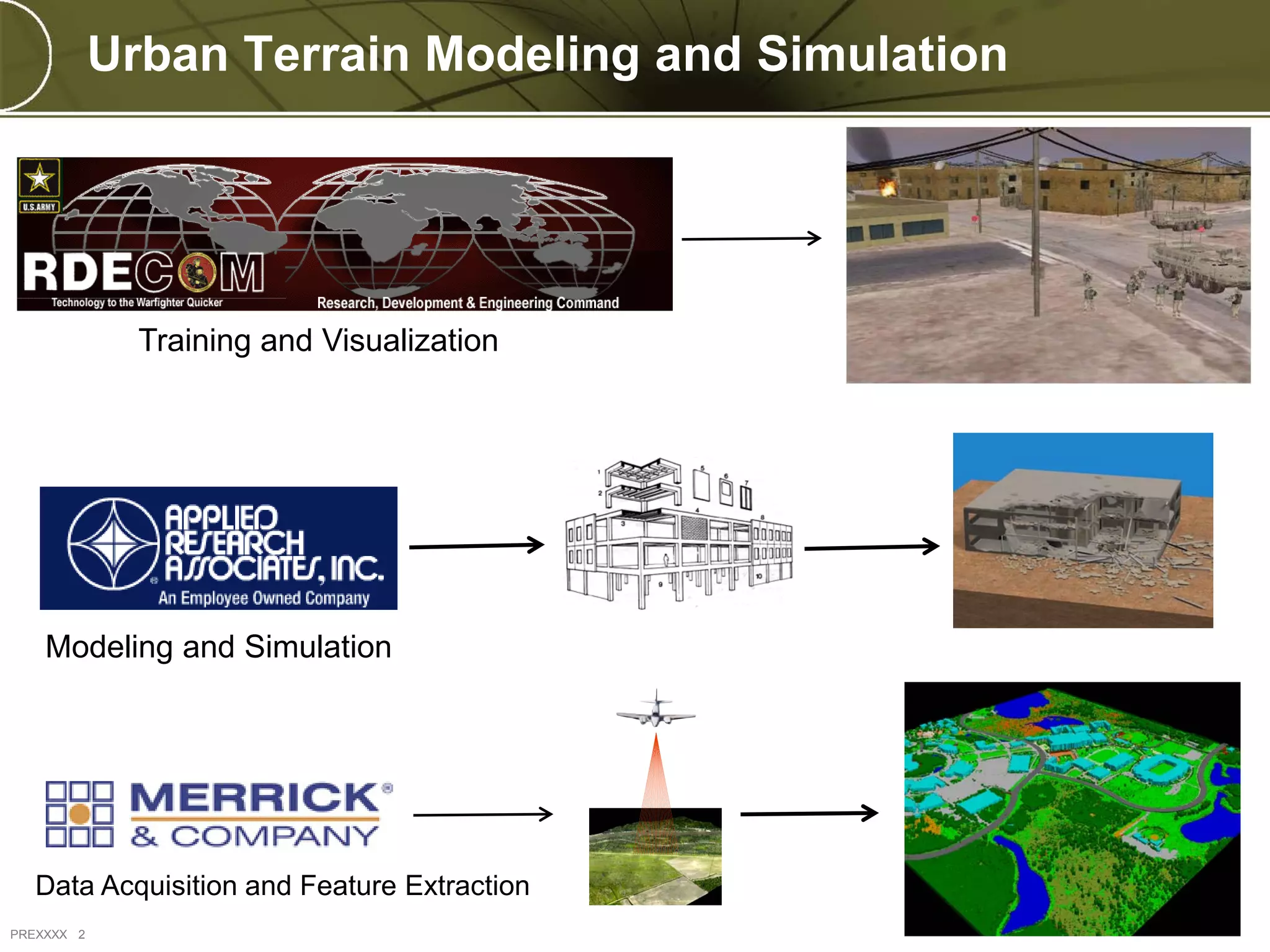
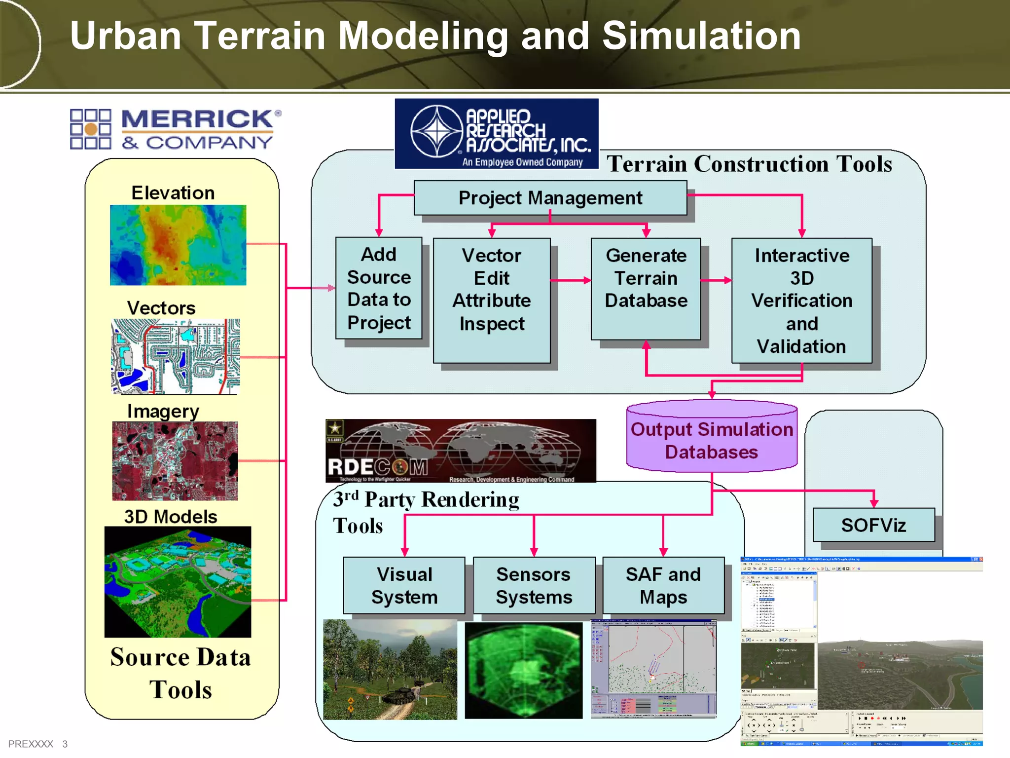
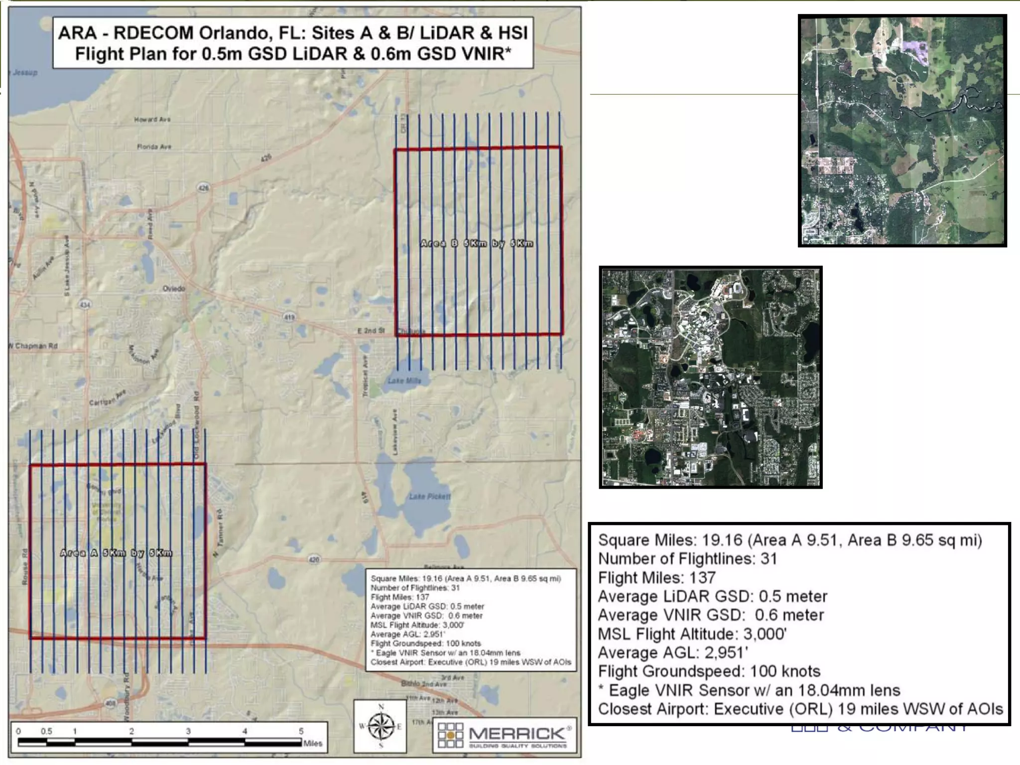
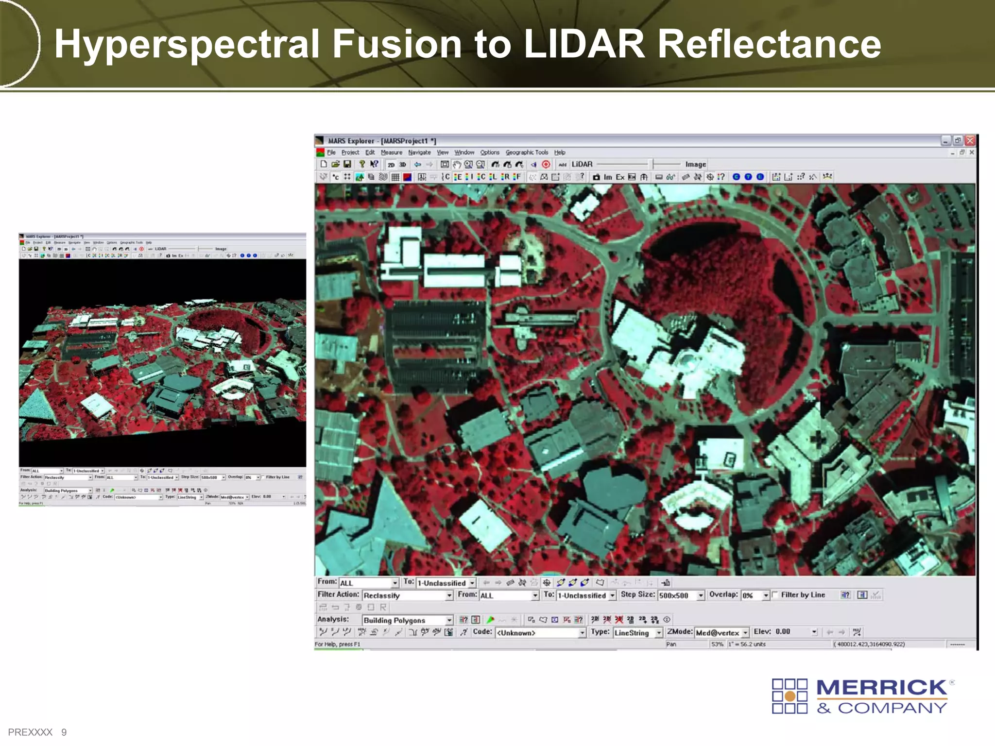
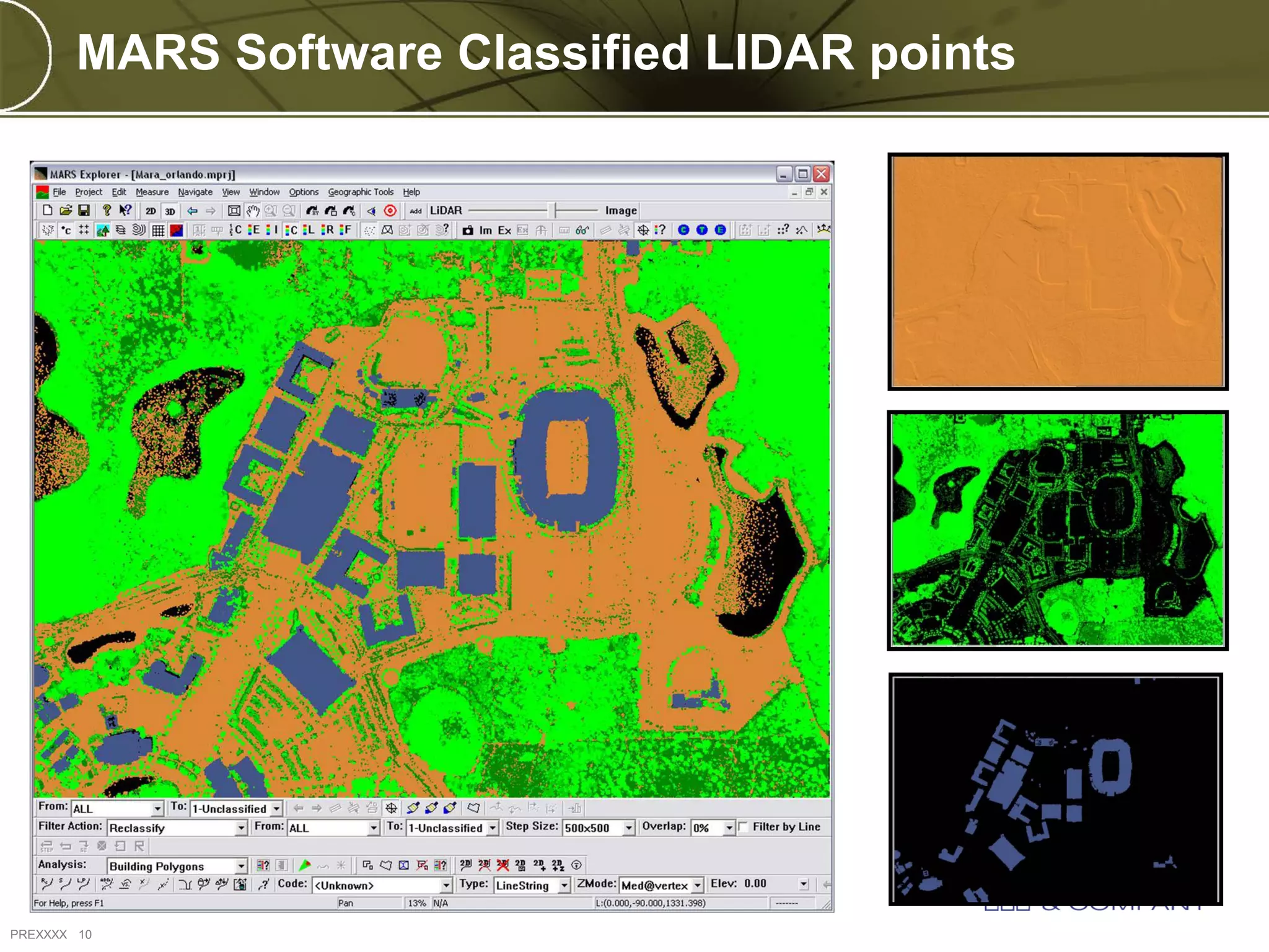
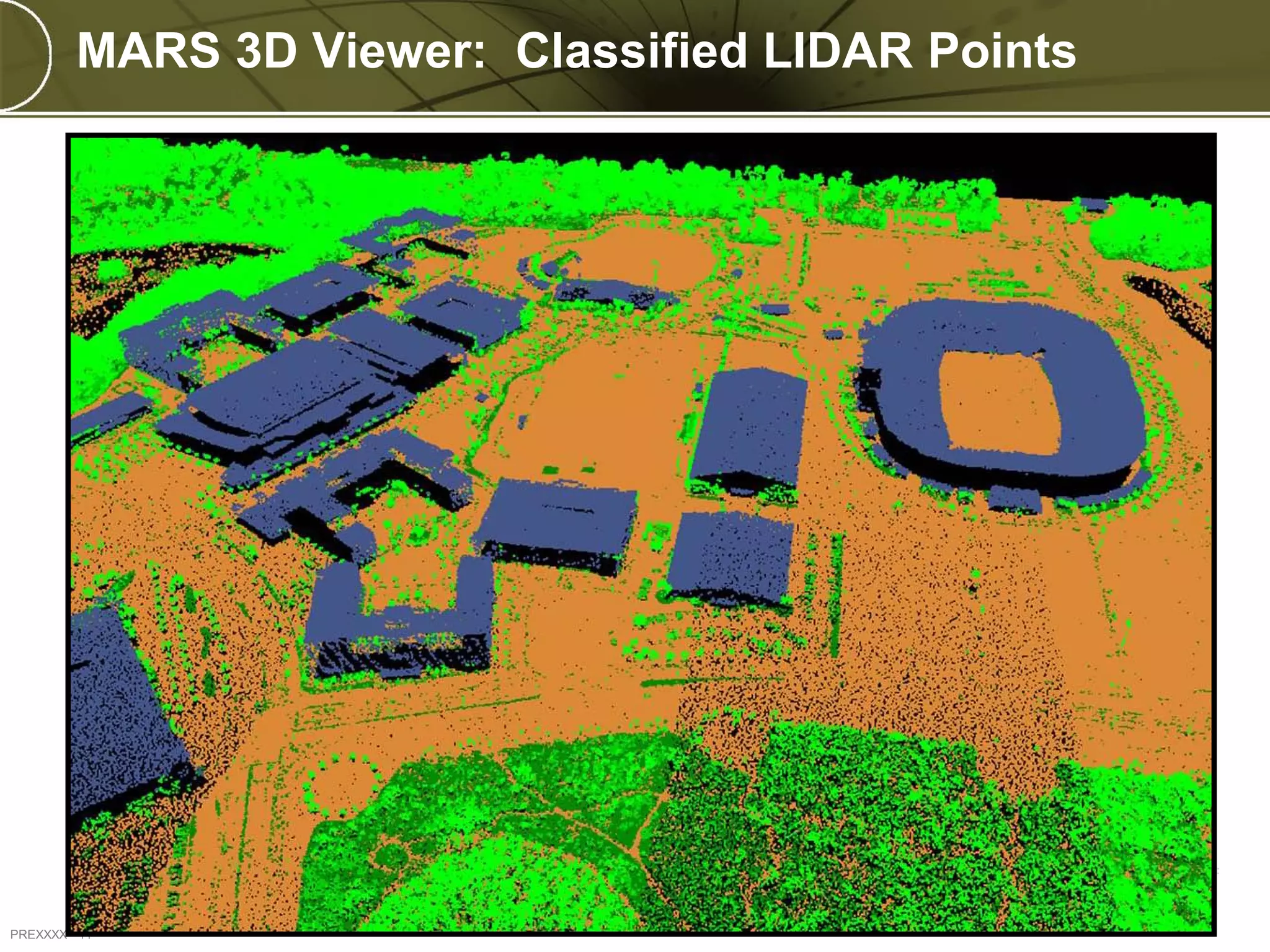
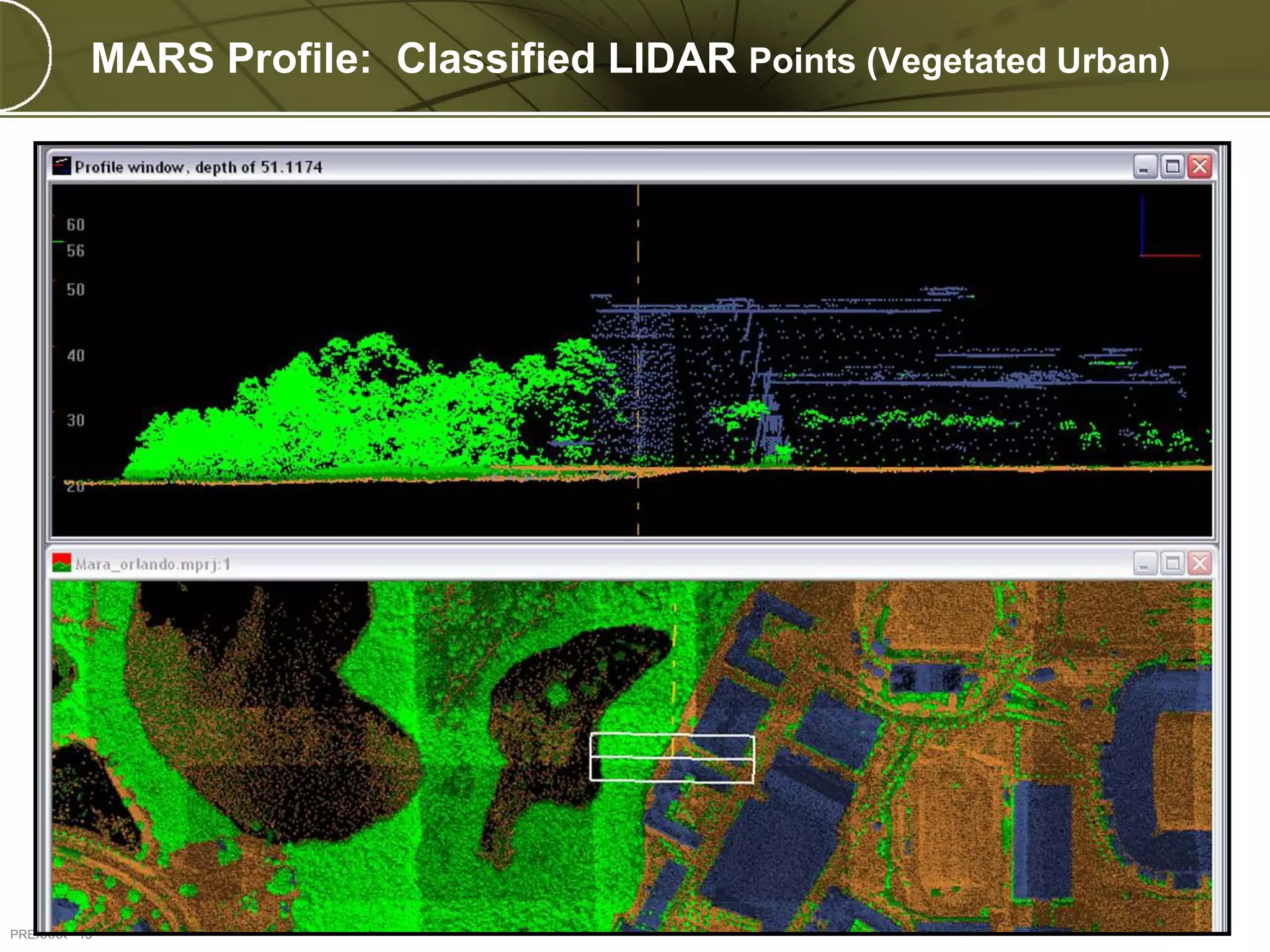
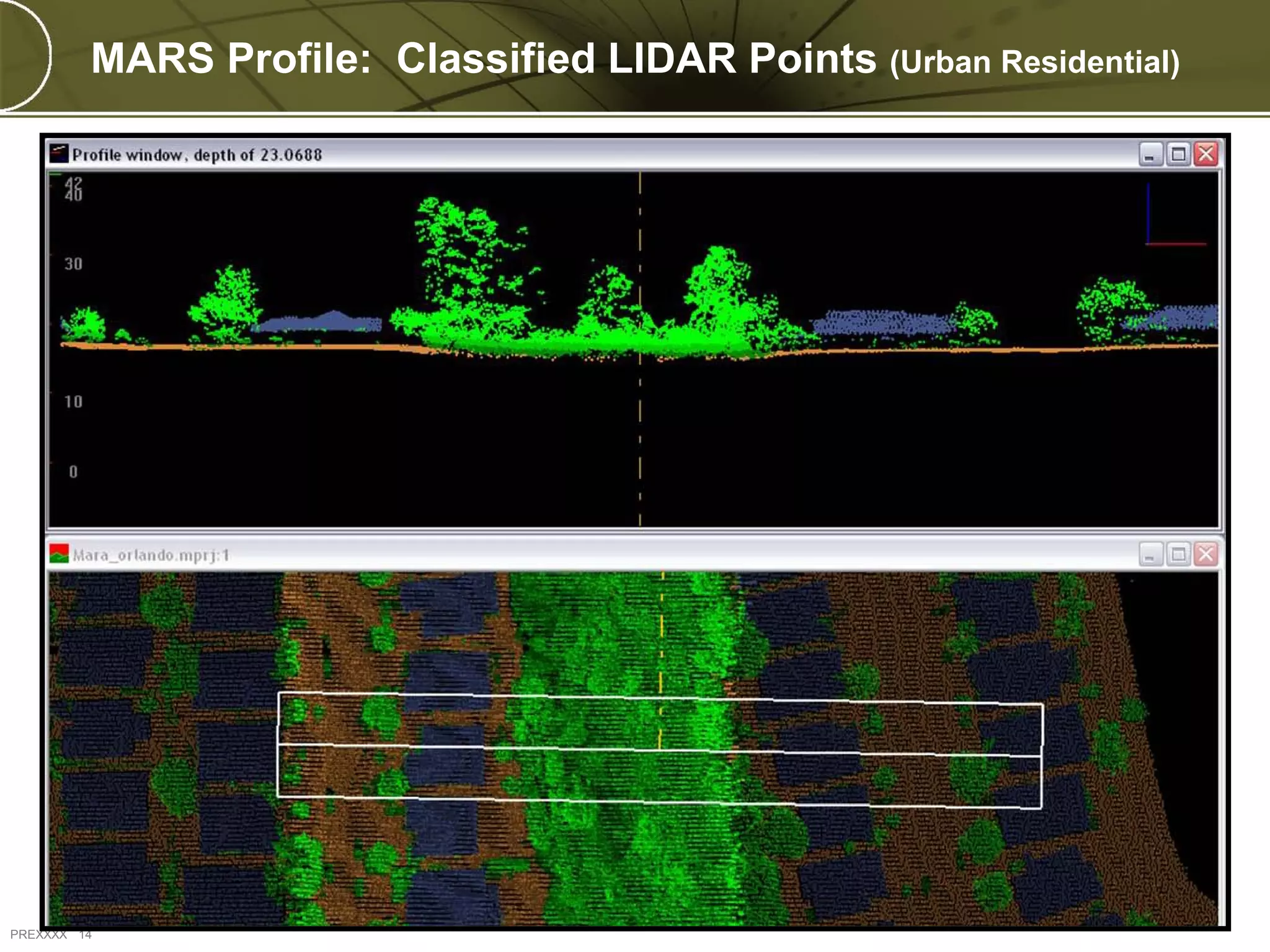
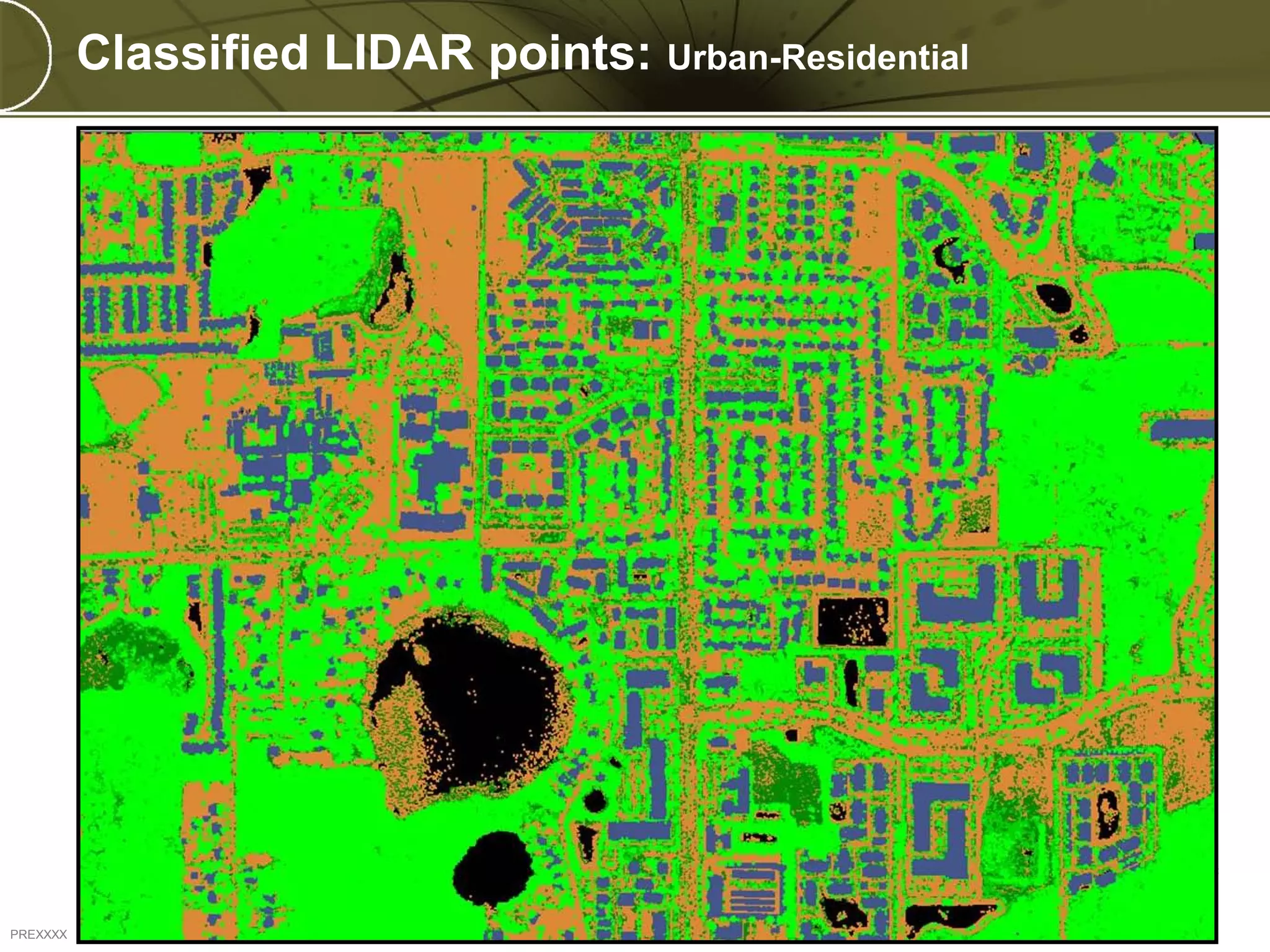
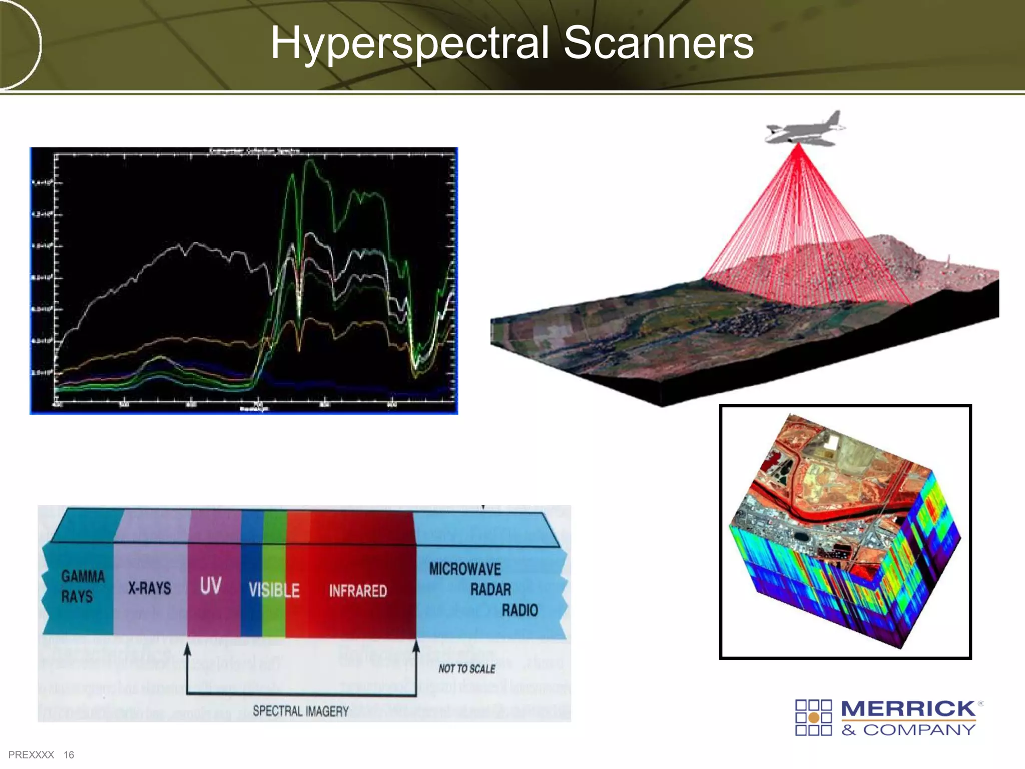
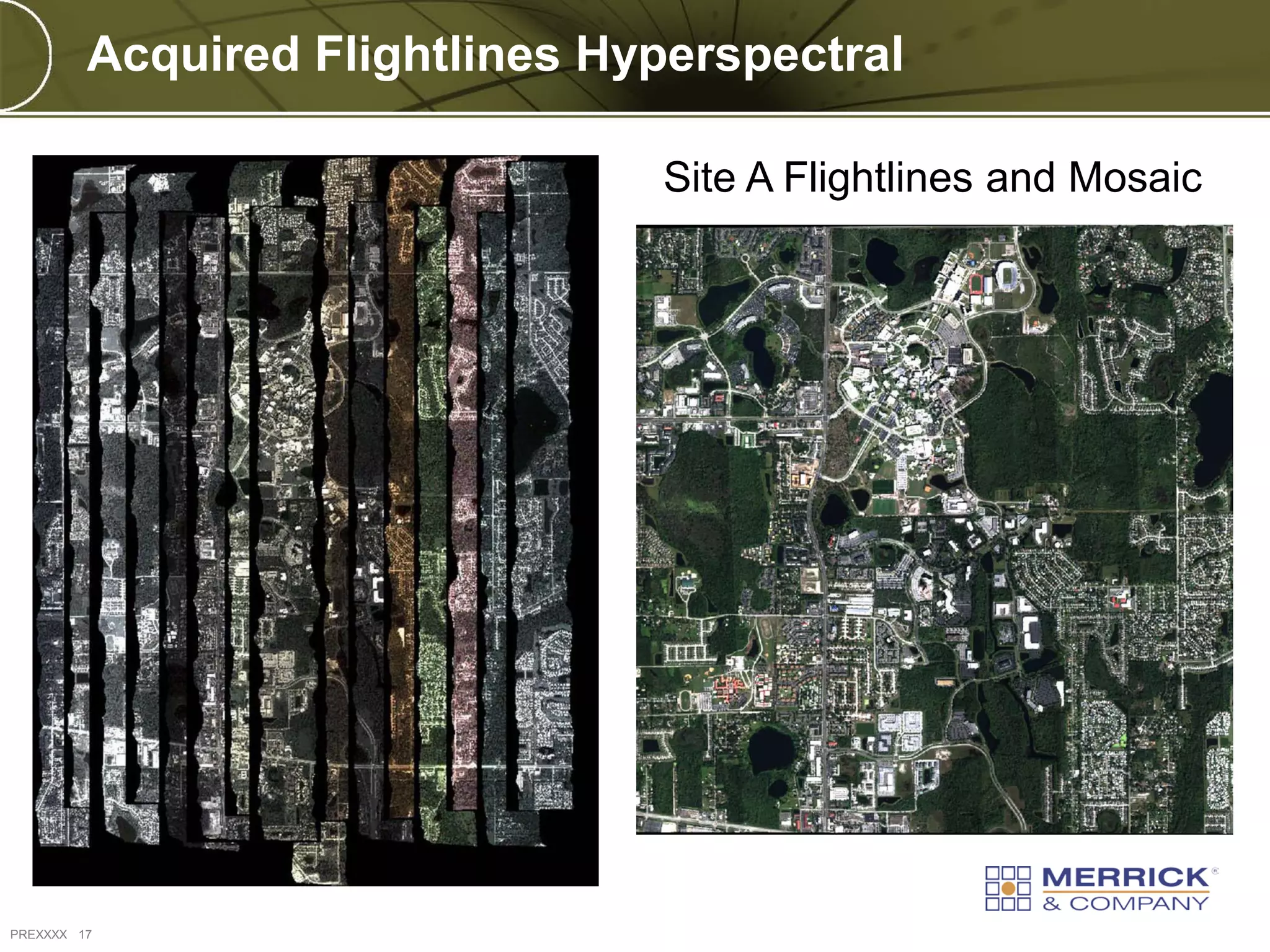
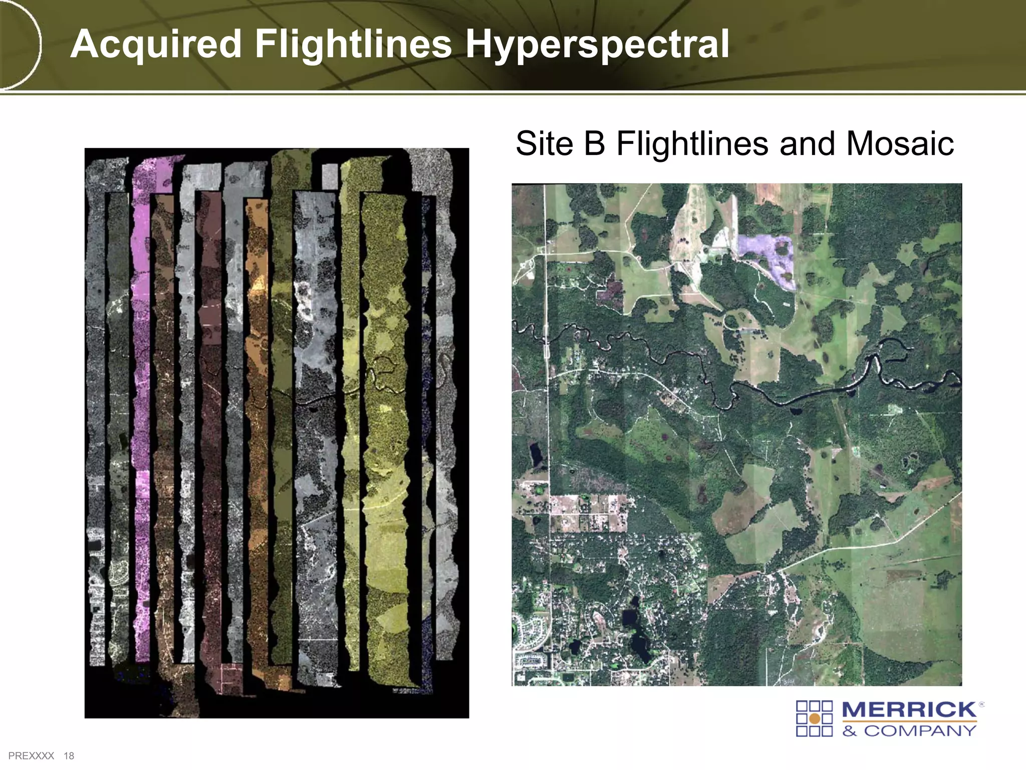
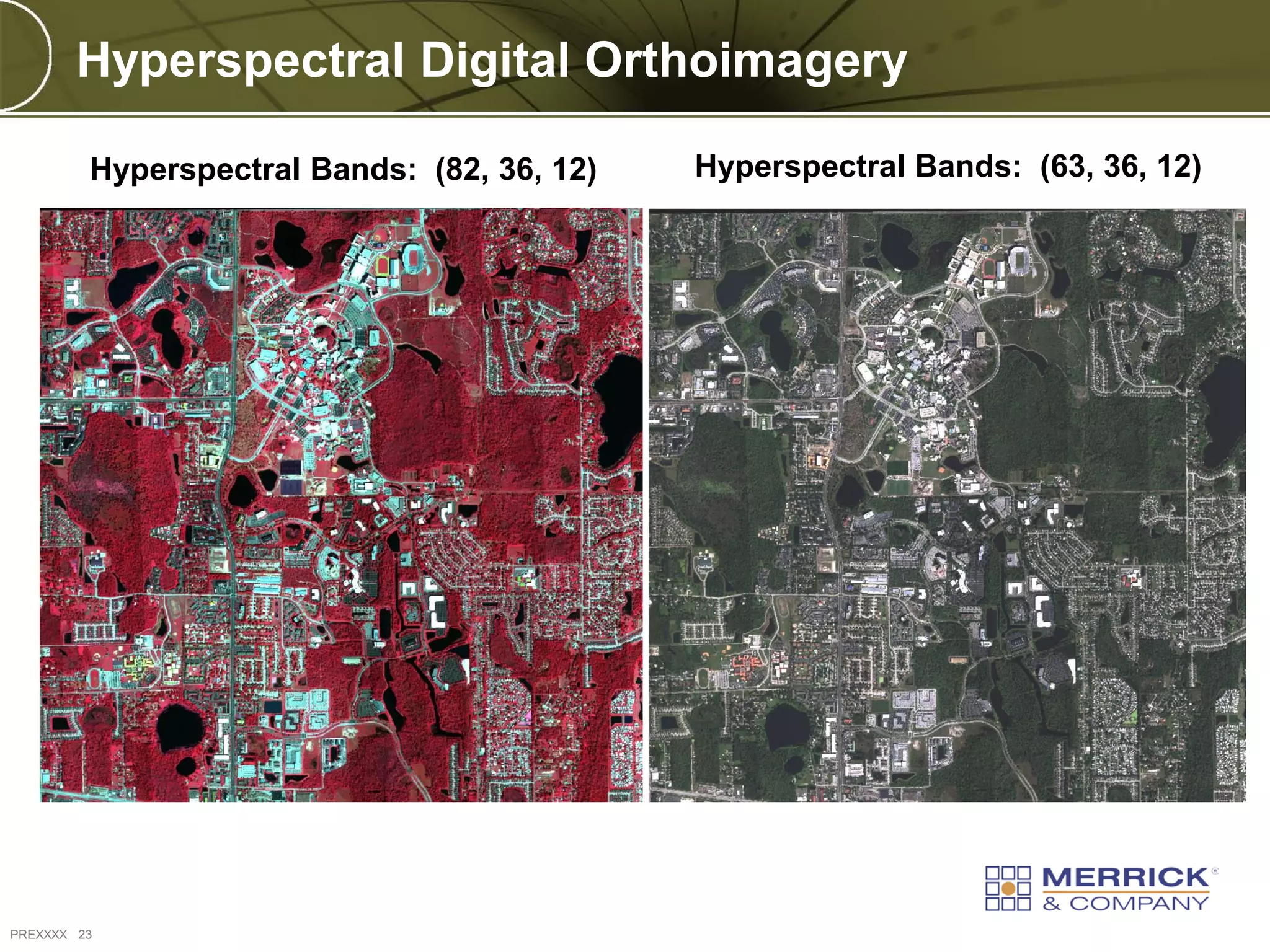
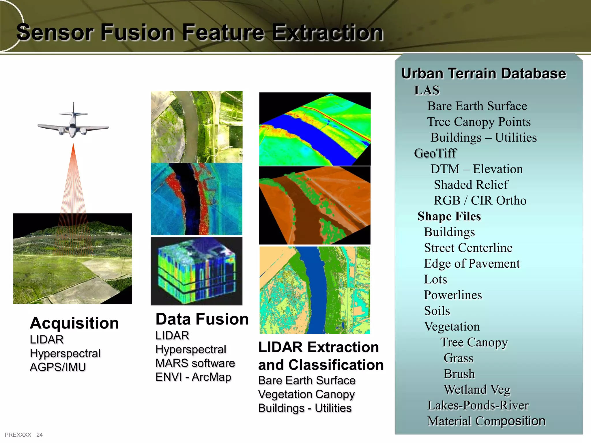
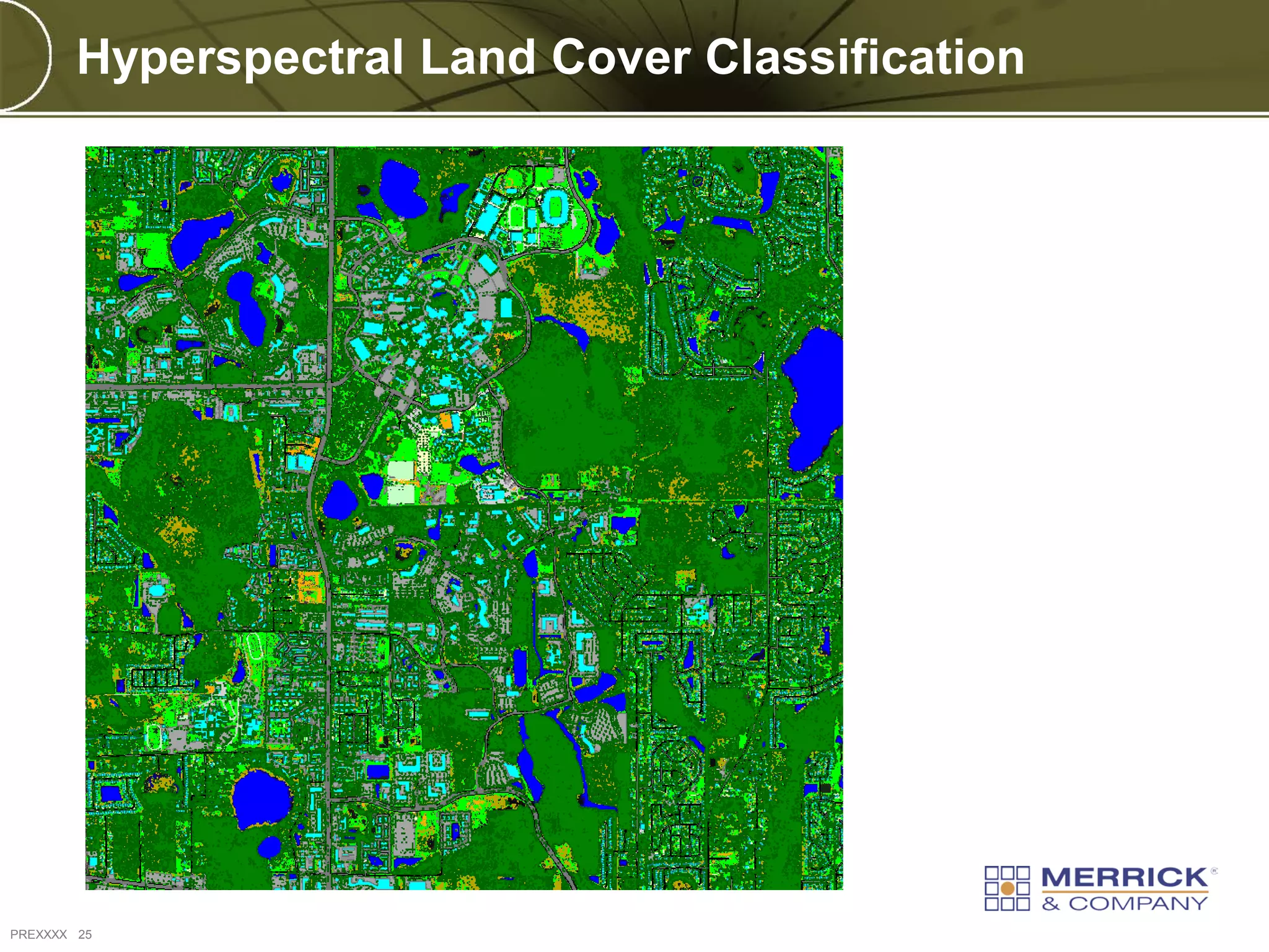
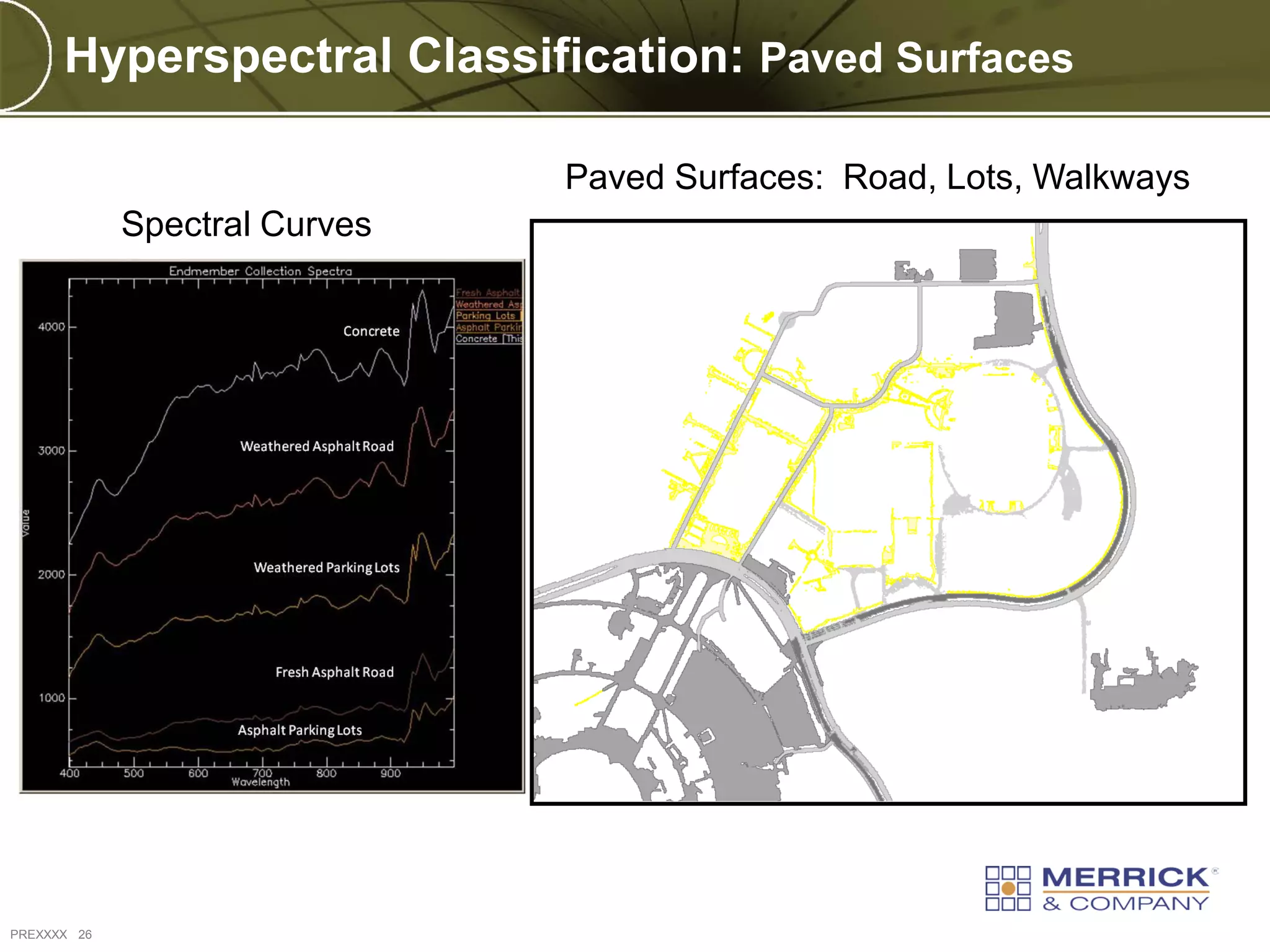
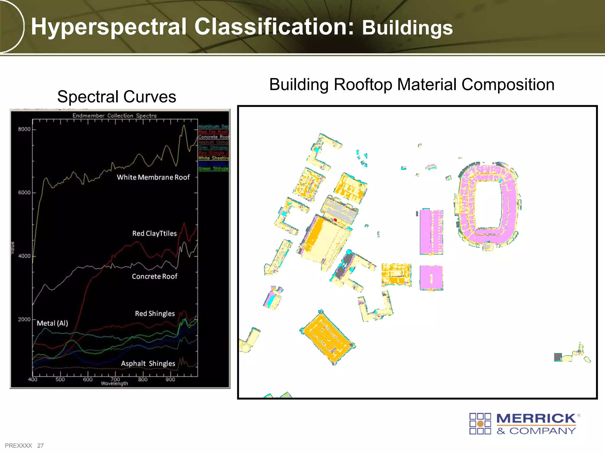
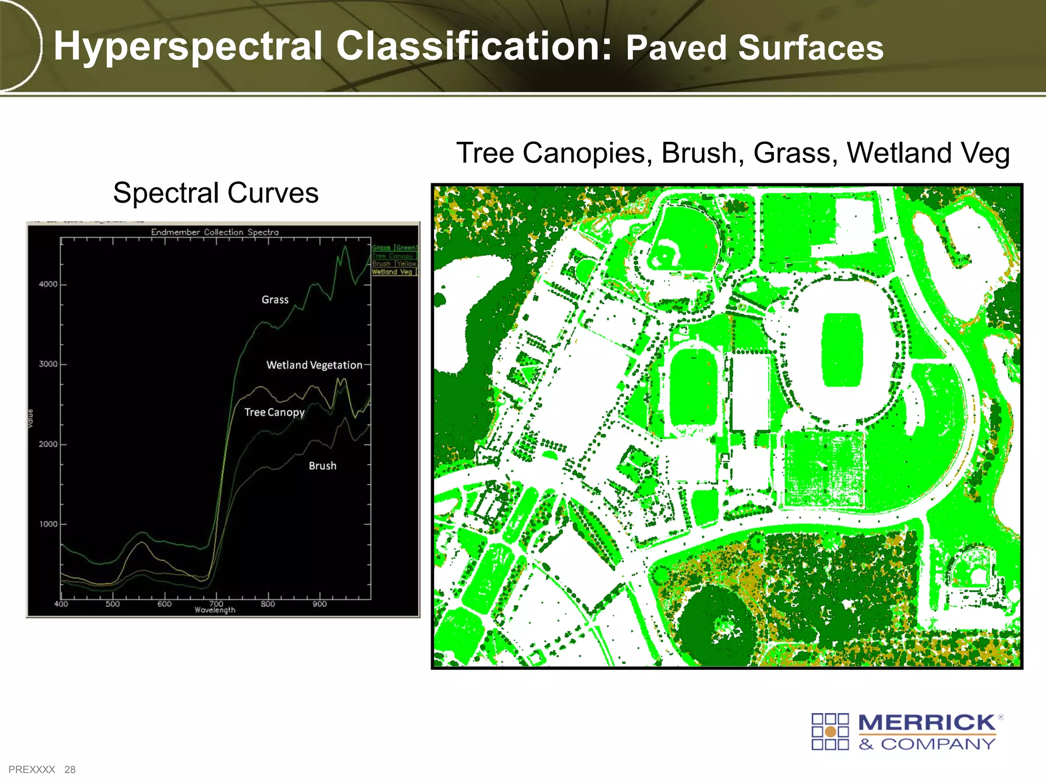
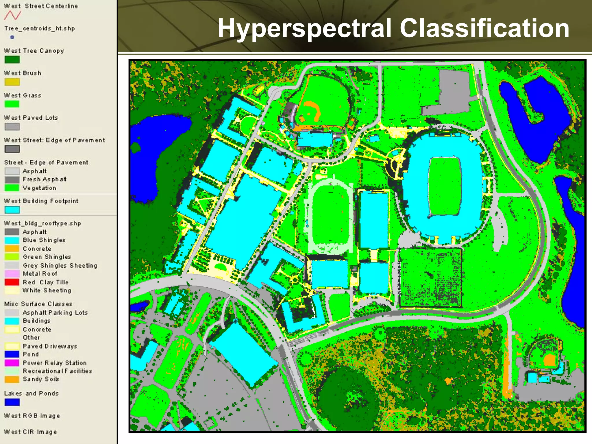
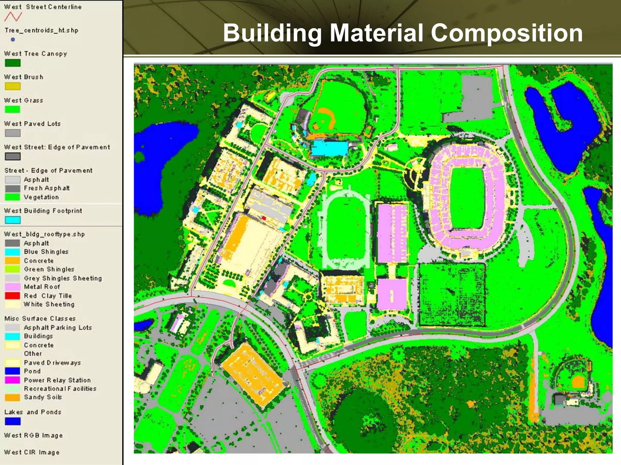
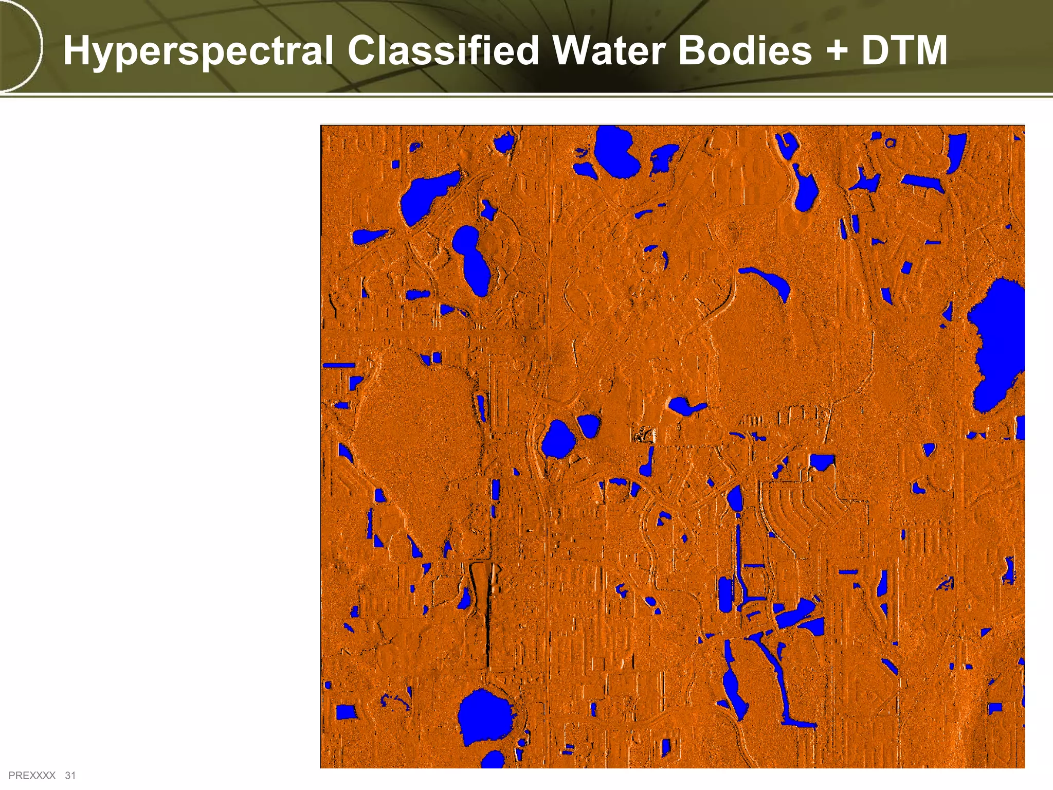
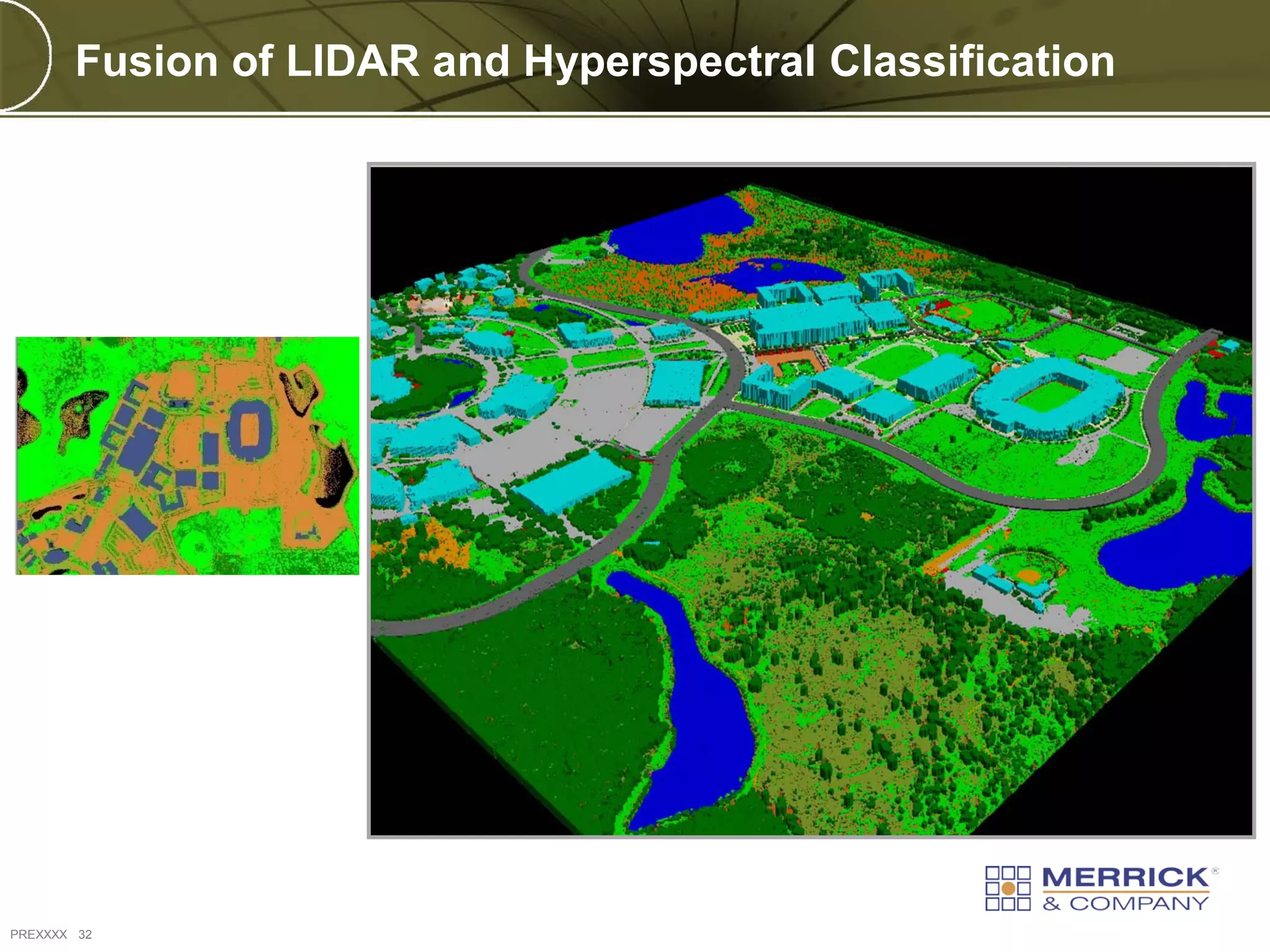
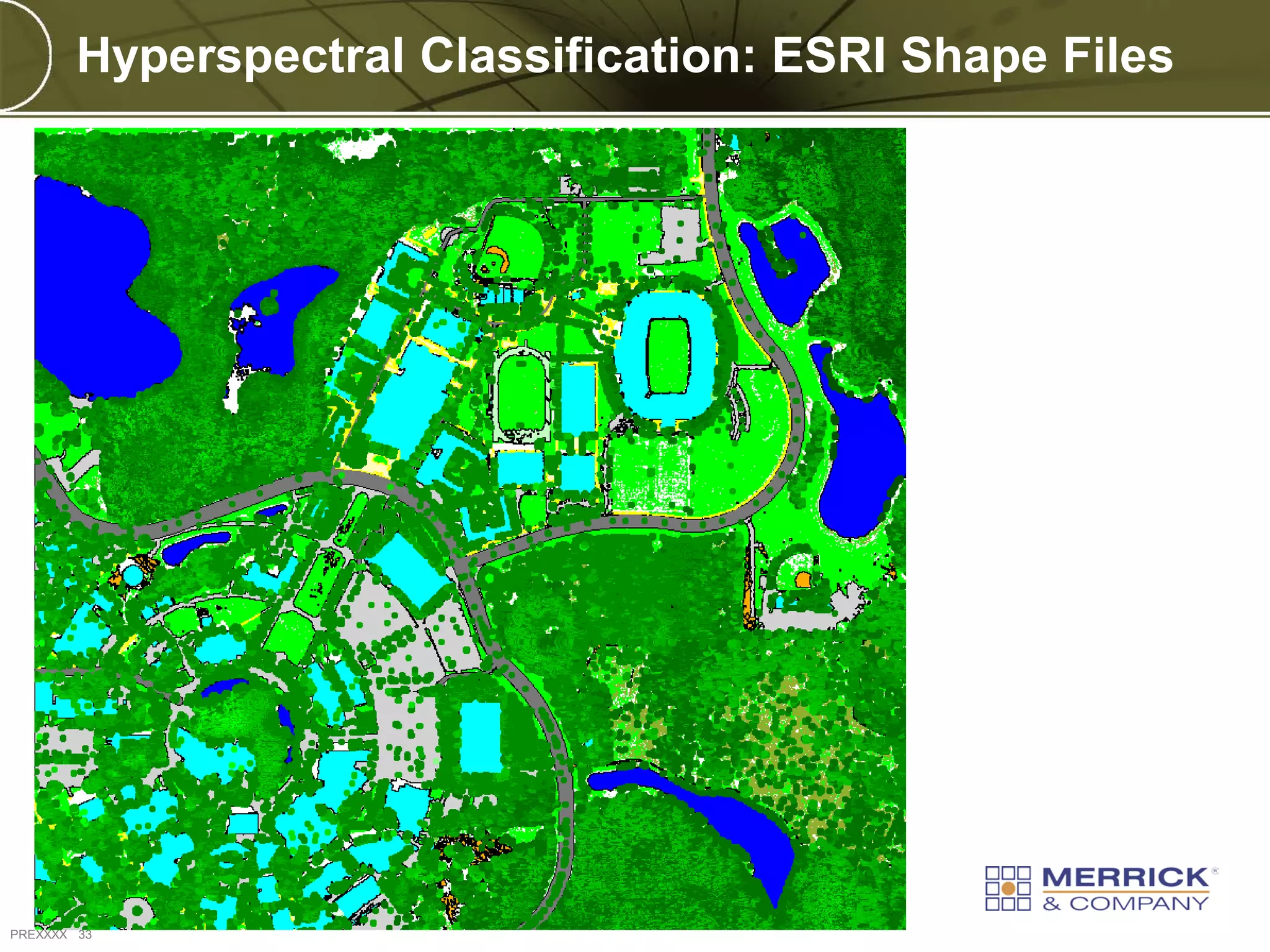
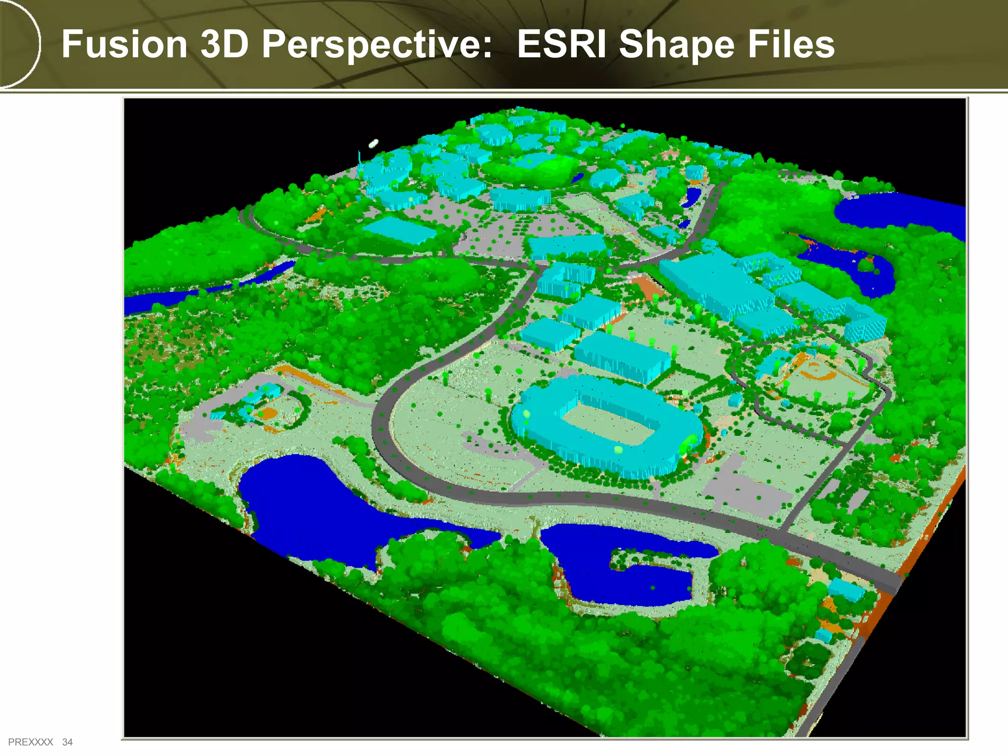
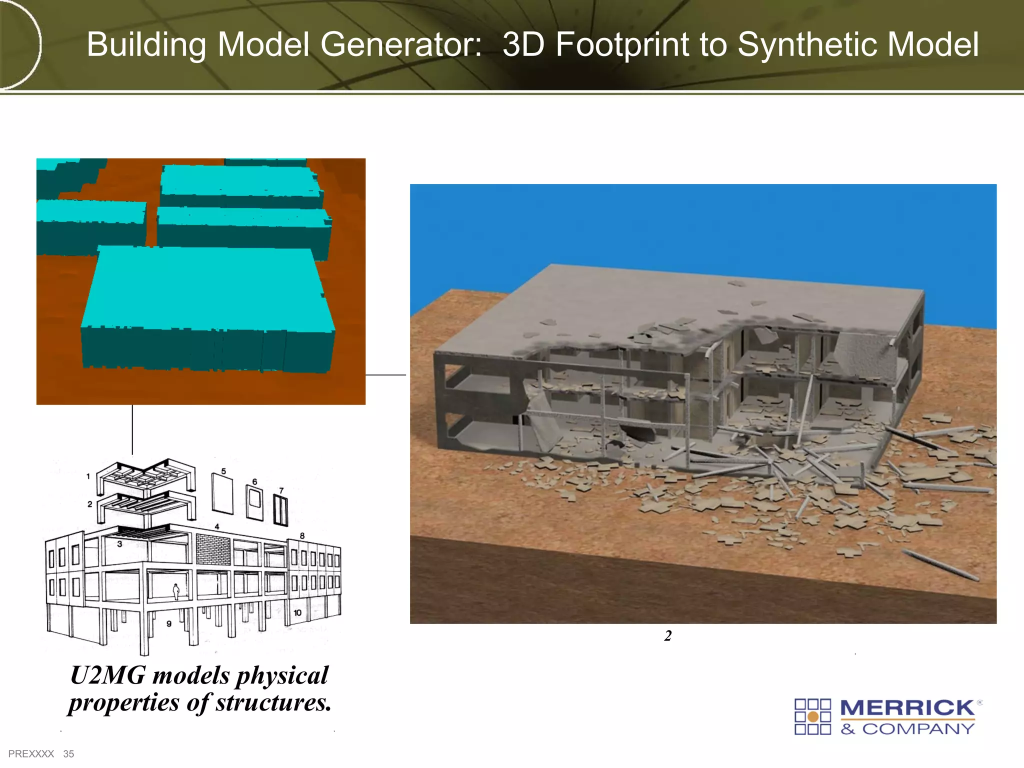
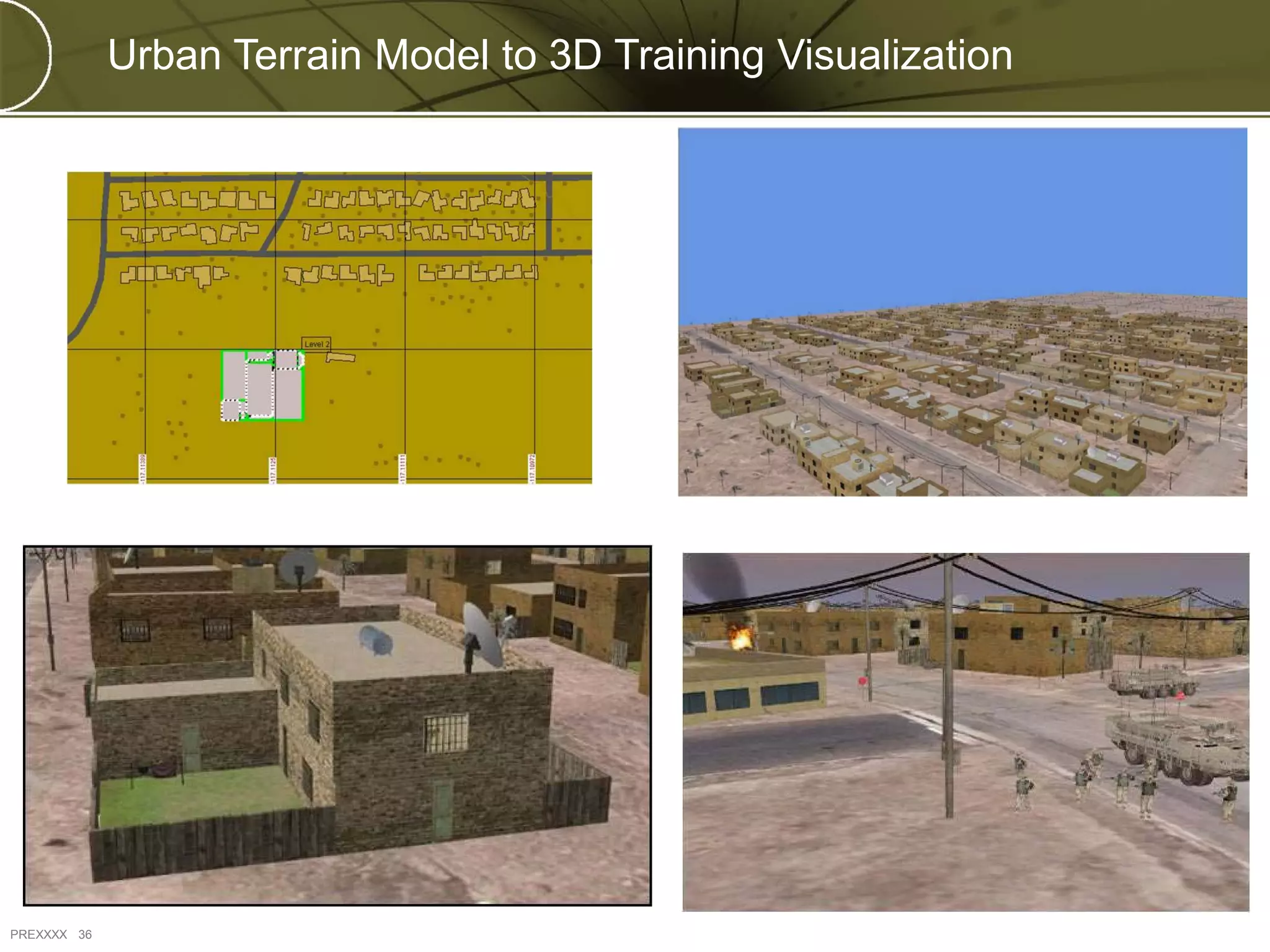
Terrain Generation:
LIDAR and Hyperspectral
      Data Fusion
 and Feature Extraction


                                                             Authors:
                                Raul Campos-Marquetti and Robert Sours

 Engineering | Architecture | Design-Build | Surveying | GeoSpatial Solutions
Urban Terrain Modeling and Simulation


              Training and Visualization


    Modeling and Simulation


   Data Acquisition and Feature Extraction
PREXXXX 2
Urban Terrain Modeling and Simulation


PREXXXX 3
PREXXXX 4
Acquisition Sensor Configuration

   LEICA         ALS-50+ LIDAR
           0.5-meter point spacing
   AISA        Eagle Hyperspectral
           0.6-meter pixel resolution
           128 spectral bands (397.8-nm to 997.96-nm)


PREXXXX 5
Acquired LIDAR Flightlines


PREXXXX 6
Mosaicked and Tiled LIDAR Flightlines

              Site A               Site B


PREXXXX 7
Raw LIDAR Reflectance (Elevation)


PREXXXX 8
Hyperspectral Fusion to LIDAR Reflectance


PREXXXX 9
MARS Software Classified LIDAR points


PREXXXX 10
MARS 3D Viewer: Classified LIDAR Points


PREXXXX 11
MARS Profile: Classified LIDAR Points (Urban)


PREXXXX 12
MARS Profile: Classified LIDAR Points (Vegetated Urban)


PREXXXX 13
MARS Profile: Classified LIDAR Points (Urban Residential)


PREXXXX 14
Classified LIDAR points: Urban-Residential


PREXXXX 15
Hyperspectral Scanners


PREXXXX 16
Acquired Flightlines Hyperspectral

                                Site A Flightlines and Mosaic


PREXXXX 17
Acquired Flightlines Hyperspectral

                               Site B Flightlines and Mosaic


PREXXXX 18
Atmospheric Correction: Radiative Transfer Model


                        Rsp(x,y,w) = [ Rdn(x,y,w) * Gain(W) ] + Offset(w)


             Rsurf(x,y,w) = [ R0(x,y,w) / {Rsol(w) x T(w) x cos(theta)} ] – Rpath(w)

    where:

    Rsp:          Spectral Radiance at sensor
    Rdn:          Grey Scale Value
    Gain:         Measure of max radiance instrument response
    Offset:       Dark Current Radiance (measure of internal system background noise)
    Rsurf:        Surface Reflectance
    Ro:           Observed Radiance at Sensor
    Rsol:         Solar Irradiance above the earth’s atmosphere
    T:            total Atmospheric Transmittance
    Rpath:        Path Radiance
    (theta):     Incidence Angle
    (x,y):         Pixel x,y, cooridnates
    W:             Wavelength


PREXXXX 19
Atmospheric Correction Model Input Parameters
        Input Image file: filename: 1013-1043_rad.dat
        Image Dimension (bands,samples,lines,offset): (128, 965, 7208, 0)
        Latitude / Longitude (deg, min, sec): ( 28.5874 0.0 0.0 N / -81.2243 0.0 0.0 W)
        Image date (day, month, year): 13 10 2009
        Image average time (UTC) (hour, minute, second): 14 45 19
        Image mean elevation (meters): -11
        Image acquisition altitude (kilometers): 0.8855


        Atmospheric Model (1=ml summer, 2=ml winter, 3=tropic): 1
        Derive water vapor (0=no, 1=940, 2=1140, 3=both, 4=820): 1
        Path Radiance in water vapor fit (0=no, 1=yes): 1
        Image Atmosphere Visibility(5 to 250 kilometers): 30
        Estimated Visibility (1=yes, 0=no): 1


        Image Spectral Calibration file: Spectral_Calibration_OSPREY.txt
        Artifact supression type 1,2,3 (1=yes, 0=no):1 1 1
        Gain file: Image_Gain_OSPREY.txt (0.01)
        Offset file: Image_Offset_OSPREY.txt (0.0)
        Output reflectance image file: 1013-1043_ref.dat
PREXXXX 20
Atmospheric Correction: Concrete-Asphalt Spectral Curves


PREXXXX 21
Atmospheric Correction: Vegetation - Grass


PREXXXX 22
Hyperspectral Digital Orthoimagery

         Hyperspectral Bands: (82, 36, 12)   Hyperspectral Bands: (63, 36, 12)


PREXXXX 23
Sensor Fusion Feature Extraction
                                                              Urban Terrain Database
                                                               LAS
                                                                 Bare Earth Surface
                                                                 Tree Canopy Points
                                                                 Buildings – Utilities
                                                               GeoTiff
                                                                 DTM – Elevation
                                                                  Shaded Relief
                                                                  RGB / CIR Ortho
                                                               Shape Files
                                                                Buildings
                                                                Street Centerline
                                                                Edge of Pavement
                                                                Lots
                                                                Powerlines
                                                                Soils
      Acquisition     Data Fusion                               Vegetation
      LIDAR           LIDAR
                                      LIDAR Extraction             Tree Canopy
      Hyperspectral   Hyperspectral
                      MARS software                                 Grass
      AGPS/IMU                        and Classification
                      ENVI - ArcMap   Bare Earth Surface
                                                                    Brush
                                      Vegetation Canopy             Wetland Veg
                                      Buildings - Utilities      Lakes-Ponds-River
                                                                 Material Composition
PREXXXX 24
Hyperspectral Land Cover Classification


PREXXXX 25
Hyperspectral Classification: Paved Surfaces

                               Paved Surfaces: Road, Lots, Walkways
             Spectral Curves


PREXXXX 26
Hyperspectral Classification: Buildings

                               Building Rooftop Material Composition
             Spectral Curves


PREXXXX 27
Hyperspectral Classification: Paved Surfaces

                               Tree Canopies, Brush, Grass, Wetland Veg
             Spectral Curves


PREXXXX 28
Hyperspectral Classification


PREXXXX 29
Building Material Composition


PREXXXX 30
Hyperspectral Classified Water Bodies + DTM


PREXXXX 31
Fusion of LIDAR and Hyperspectral Classification


PREXXXX 32
Hyperspectral Classification: ESRI Shape Files


PREXXXX 33
Fusion 3D Perspective: ESRI Shape Files


PREXXXX 34
Building Model Generator: 3D Footprint to Synthetic Model


                                                 2

         U2MG models physical
         properties of structures.
PREXXXX 35
Urban Terrain Model to 3D Training Visualization


PREXXXX 36
Conclusion

            The fusion of LIDAR and Hyperspectral data provides a means by
             which to efficiently generate the base data for 3D Urban Databases
            Provides Real World Locations and Feature Classes
                Real World Coordinates for features (x,y,z)
                Land Cover and Land Use Classes
                Physical morphology of features and Attribute extraction
                Material Composition of feature infrastructure
                Generation of 3D feature Objects for use in Modeling & Simulation
                 environments, providing realistic training scenarios


                        Raul Campos-Marquetti / Remote Sensing Solutions Manager
                                   Email: rcmarquetti@merrick.com


PREXXXX 37

Lidar hsi datafusion ilmf 2010

  • 1.
    Terrain Generation: LIDAR andHyperspectral Data Fusion and Feature Extraction Authors: Raul Campos-Marquetti and Robert Sours Engineering | Architecture | Design-Build | Surveying | GeoSpatial Solutions
  • 2.
    Urban Terrain Modelingand Simulation Training and Visualization Modeling and Simulation Data Acquisition and Feature Extraction PREXXXX 2
  • 3.
    Urban Terrain Modelingand Simulation PREXXXX 3
  • 4.
  • 5.
    Acquisition Sensor Configuration  LEICA ALS-50+ LIDAR  0.5-meter point spacing  AISA Eagle Hyperspectral  0.6-meter pixel resolution  128 spectral bands (397.8-nm to 997.96-nm) PREXXXX 5
  • 6.
  • 7.
    Mosaicked and TiledLIDAR Flightlines Site A Site B PREXXXX 7
  • 8.
    Raw LIDAR Reflectance(Elevation) PREXXXX 8
  • 9.
    Hyperspectral Fusion toLIDAR Reflectance PREXXXX 9
  • 10.
    MARS Software ClassifiedLIDAR points PREXXXX 10
  • 11.
    MARS 3D Viewer:Classified LIDAR Points PREXXXX 11
  • 12.
    MARS Profile: ClassifiedLIDAR Points (Urban) PREXXXX 12
  • 13.
    MARS Profile: ClassifiedLIDAR Points (Vegetated Urban) PREXXXX 13
  • 14.
    MARS Profile: ClassifiedLIDAR Points (Urban Residential) PREXXXX 14
  • 15.
    Classified LIDAR points:Urban-Residential PREXXXX 15
  • 16.
  • 17.
    Acquired Flightlines Hyperspectral Site A Flightlines and Mosaic PREXXXX 17
  • 18.
    Acquired Flightlines Hyperspectral Site B Flightlines and Mosaic PREXXXX 18
  • 19.
    Atmospheric Correction: RadiativeTransfer Model Rsp(x,y,w) = [ Rdn(x,y,w) * Gain(W) ] + Offset(w) Rsurf(x,y,w) = [ R0(x,y,w) / {Rsol(w) x T(w) x cos(theta)} ] – Rpath(w) where: Rsp: Spectral Radiance at sensor Rdn: Grey Scale Value Gain: Measure of max radiance instrument response Offset: Dark Current Radiance (measure of internal system background noise) Rsurf: Surface Reflectance Ro: Observed Radiance at Sensor Rsol: Solar Irradiance above the earth’s atmosphere T: total Atmospheric Transmittance Rpath: Path Radiance (theta): Incidence Angle (x,y): Pixel x,y, cooridnates W: Wavelength PREXXXX 19
  • 20.
    Atmospheric Correction ModelInput Parameters  Input Image file: filename: 1013-1043_rad.dat  Image Dimension (bands,samples,lines,offset): (128, 965, 7208, 0)  Latitude / Longitude (deg, min, sec): ( 28.5874 0.0 0.0 N / -81.2243 0.0 0.0 W)  Image date (day, month, year): 13 10 2009  Image average time (UTC) (hour, minute, second): 14 45 19  Image mean elevation (meters): -11  Image acquisition altitude (kilometers): 0.8855  Atmospheric Model (1=ml summer, 2=ml winter, 3=tropic): 1  Derive water vapor (0=no, 1=940, 2=1140, 3=both, 4=820): 1  Path Radiance in water vapor fit (0=no, 1=yes): 1  Image Atmosphere Visibility(5 to 250 kilometers): 30  Estimated Visibility (1=yes, 0=no): 1  Image Spectral Calibration file: Spectral_Calibration_OSPREY.txt  Artifact supression type 1,2,3 (1=yes, 0=no):1 1 1  Gain file: Image_Gain_OSPREY.txt (0.01)  Offset file: Image_Offset_OSPREY.txt (0.0)  Output reflectance image file: 1013-1043_ref.dat PREXXXX 20
  • 21.
    Atmospheric Correction: Concrete-AsphaltSpectral Curves PREXXXX 21
  • 22.
  • 23.
    Hyperspectral Digital Orthoimagery Hyperspectral Bands: (82, 36, 12) Hyperspectral Bands: (63, 36, 12) PREXXXX 23
  • 24.
    Sensor Fusion FeatureExtraction Urban Terrain Database LAS Bare Earth Surface Tree Canopy Points Buildings – Utilities GeoTiff DTM – Elevation Shaded Relief RGB / CIR Ortho Shape Files Buildings Street Centerline Edge of Pavement Lots Powerlines Soils Acquisition Data Fusion Vegetation LIDAR LIDAR LIDAR Extraction Tree Canopy Hyperspectral Hyperspectral MARS software Grass AGPS/IMU and Classification ENVI - ArcMap Bare Earth Surface Brush Vegetation Canopy Wetland Veg Buildings - Utilities Lakes-Ponds-River Material Composition PREXXXX 24
  • 25.
    Hyperspectral Land CoverClassification PREXXXX 25
  • 26.
    Hyperspectral Classification: PavedSurfaces Paved Surfaces: Road, Lots, Walkways Spectral Curves PREXXXX 26
  • 27.
    Hyperspectral Classification: Buildings Building Rooftop Material Composition Spectral Curves PREXXXX 27
  • 28.
    Hyperspectral Classification: PavedSurfaces Tree Canopies, Brush, Grass, Wetland Veg Spectral Curves PREXXXX 28
  • 29.
  • 30.
  • 31.
    Hyperspectral Classified WaterBodies + DTM PREXXXX 31
  • 32.
    Fusion of LIDARand Hyperspectral Classification PREXXXX 32
  • 33.
    Hyperspectral Classification: ESRIShape Files PREXXXX 33
  • 34.
    Fusion 3D Perspective:ESRI Shape Files PREXXXX 34
  • 35.
    Building Model Generator:3D Footprint to Synthetic Model 2 U2MG models physical properties of structures. PREXXXX 35
  • 36.
    Urban Terrain Modelto 3D Training Visualization PREXXXX 36
  • 37.
    Conclusion  The fusion of LIDAR and Hyperspectral data provides a means by which to efficiently generate the base data for 3D Urban Databases  Provides Real World Locations and Feature Classes  Real World Coordinates for features (x,y,z)  Land Cover and Land Use Classes  Physical morphology of features and Attribute extraction  Material Composition of feature infrastructure  Generation of 3D feature Objects for use in Modeling & Simulation environments, providing realistic training scenarios Raul Campos-Marquetti / Remote Sensing Solutions Manager Email: rcmarquetti@merrick.com PREXXXX 37