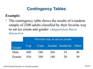
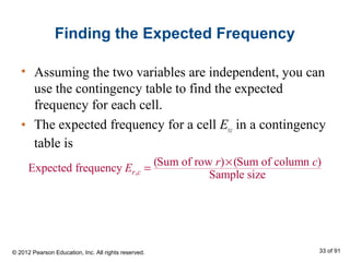
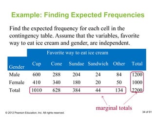
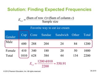
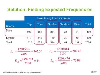
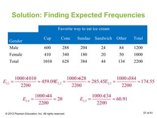
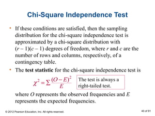
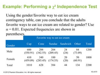
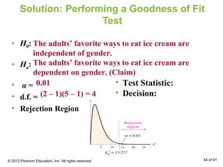
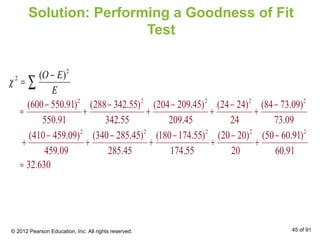
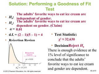
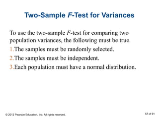
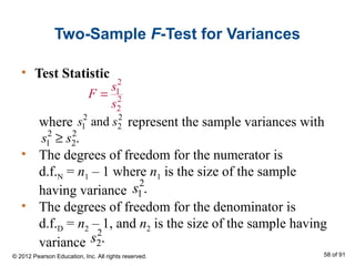
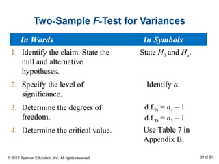
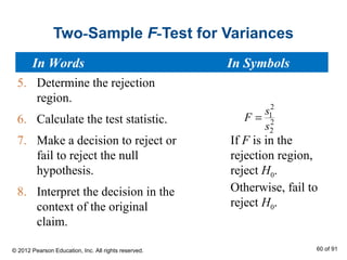
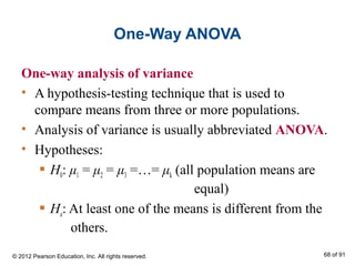
This document outlines how to perform a chi-square test of independence using a contingency table. It explains that a contingency table displays the observed frequencies of two variables arranged in rows and columns. Expected frequencies are calculated for each cell assuming independence by multiplying the corresponding row and column totals and dividing by the sample size. A chi-square test can then determine if the observed frequencies differ significantly from the expected frequencies under independence.


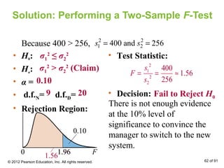

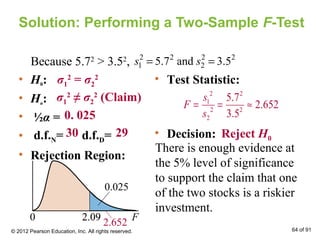


![Goodness of Fit [Autosaved] power point presentation](https://cdn.slidesharecdn.com/ss_thumbnails/goodnessoffitautosaved-241112161427-2da4f412-thumbnail.jpg?width=640&height=640&fit=bounds)


