Les5e ppt 08

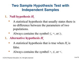
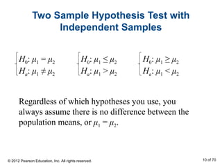
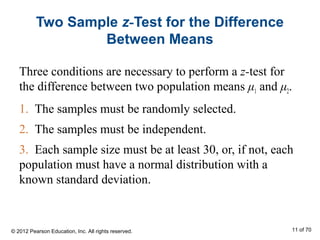
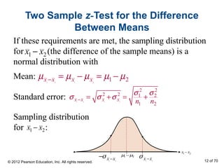
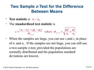
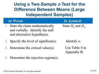
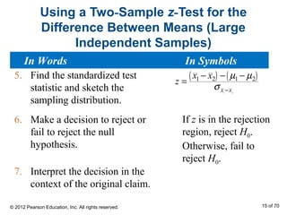
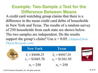
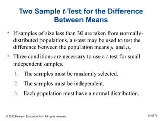
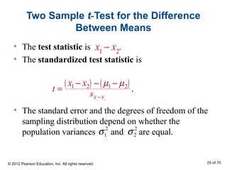
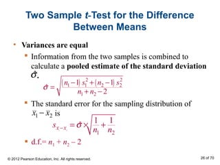
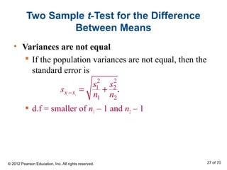
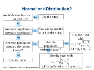
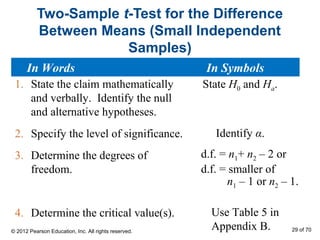
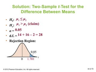
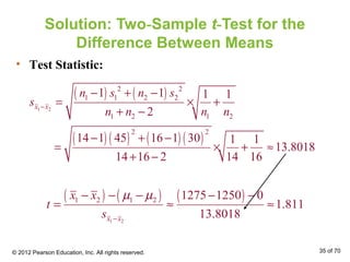
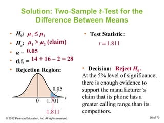
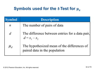
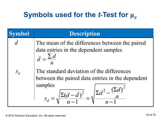
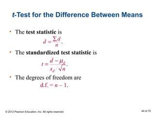
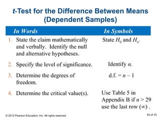
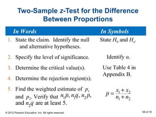
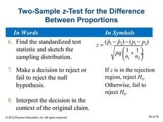
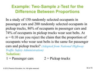
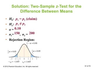
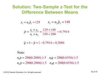
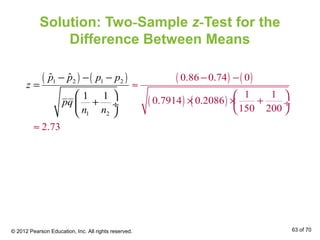
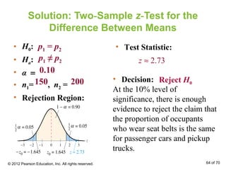
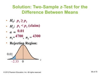
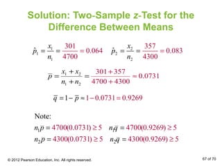
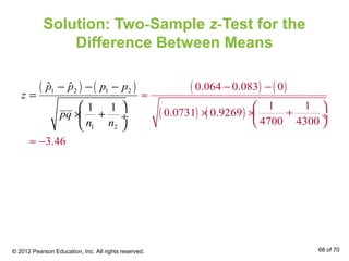
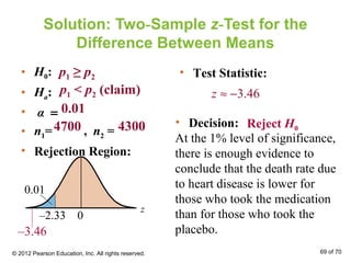
Chapter
Hypothesis Testing
with Two Samples
1 of 70
8
© 2012 Pearson Education, Inc.
All rights reserved.

Chapter Outline
• 8.1 Testing the Difference Between Means (Large
Independent Samples)
• 8.2 Testing the Difference Between Means (Small
• 8.3 Testing the Difference Between Means
(Dependent Samples)
• 8.4 Testing the Difference Between Proportions
© 2012 Pearson Education, Inc. All rights reserved. 2 of 70

Section 8.1
Testing the Difference Between
Means (Large Independent Samples)

Section 8.1 Objectives
• Determine whether two samples are independent or
dependent
• Perform a two-sample z-test for the difference
between two means μ1 and μ2 using large independent
samples

Two Sample Hypothesis Test
• Compares two parameters from two populations.
• Sampling methods:
 Independent Samples
• The sample selected from one population is not
related to the sample selected from the second
population.
 Dependent Samples (paired or matched samples)
• Each member of one sample corresponds to a
member of the other sample.

Independent and Dependent Samples
Independent Samples
Sample 1 Sample 2
Dependent Samples
Sample 1 Sample 2

Example: Independent and Dependent
Samples
Classify the pair of samples as independent or
dependent.
• Sample 1: Weights of 65 college students before their
freshman year begins.
• Sample 2: Weights of the same 65 college students
after their freshmen year.
Solution:
Dependent Samples (The samples can be paired with
respect to each student)

Example: Independent and Dependent
Samples
Classify the pair of samples as independent or dependent.
• Sample 1: Scores for 38 adults males on a psycho-
logical screening test for attention-deficit hyperactivity
disorder.
• Sample 2: Scores for 50 adult females on a psycho-
logical screening test for attention-deficit hyperactivity
disorder.
Solution:
Independent Samples (Not possible to form a pairing
between the members of the samples; the sample sizes
are different, and the data represent scores for different
individuals.)

Two Sample Hypothesis Test with
Independent Samples
1. Null hypothesis H0
 A statistical hypothesis that usually states there is
no difference between the parameters of two
populations.
 Always contains the symbol ≤, =, or ≥.
1. Alternative hypothesis Ha
 A statistical hypothesis that is true when H0 is
false.
 Always contains the symbol >, ≠, or <.

Two Sample Hypothesis Test with
Independent Samples
H0: μ1 = μ2
Ha: μ1 ≠ μ2
H0: μ1 ≤ μ2
Ha: μ1 > μ2
H0: μ1 ≥ μ2
Ha: μ1 < μ2
Regardless of which hypotheses you use, you
always assume there is no difference between the
population means, or μ1 = μ2.

Two Sample z-Test for the Difference
Between Means
Three conditions are necessary to perform a z-test for
the difference between two population means μ1 and μ2.
1. The samples must be randomly selected.
2. The samples must be independent.
3. Each sample size must be at least 30, or, if not, each
population must have a normal distribution with a
known standard deviation.

Between Means
If these requirements are met, the sampling distribution
for (the difference of the sample means) is a
normal distribution with
1 2 1 2
1 2x x x xµ µ µ µ µ− = − = −
1 2x x−
1 2 1 2
2 2
2 2 1 2
1 2
x x x x n n
σ σ
σ σ σ− = + = +
Sampling distribution
for :1 2x x−
Mean:
Standard error:
1 2x x−
1 2µ µ−
1 2
x x−−σ 1 2
x x−σ

Between Means
• Test statistic is .
• The standardized test statistic is
• When the samples are large, you can use s1and s2 in place
of σ1 and σ2. If the samples are not large, you can still use
a two-sample z-test, provided the populations are
normally distributed and the population standard
deviations are known.
( ) ( )
1 2
1 2
2 2
1 2 1 2 1 2
1 2
.x x
x x
x x
z where
n n
µ µ σ σ
σ
σ −
−
− − −
= = +
1 2x x−

Using a Two-Sample z-Test for the
Difference Between Means (Large
1. State the claim mathematically
and verbally. Identify the null
and alternative hypotheses.
2. Specify the level of significance.
3. Determine the critical value(s).
4. Determine the rejection region(s).
State H0 and Ha.
Identify α.
Use Table 4 in
Appendix B.
In Words In Symbols

Using a Two-Sample z-Test for the
Difference Between Means (Large
5. Find the standardized test
statistic and sketch the
sampling distribution.
6. Make a decision to reject or
fail to reject the null
hypothesis.
7. Interpret the decision in the
context of the original claim.
( ) ( )
1 2
1 2 1 2
x x
x x
z
µ µ
σ −
− − −
=
If z is in the rejection
region, reject H0.
Otherwise, fail to
reject H0.
In Words In Symbols

Example: Two-Sample z-Test for the
Difference Between Means
A credit card watchdog group claims that there is a
difference in the mean credit card debts of households
in New York and Texas. The results of a random survey
of 250 households from each state are shown below.
The two samples are independent. Do the results
support the group’s claim? Use α = 0.05. (Adapted from
PlasticRewards.com)
New York Texas
s1 = $1045.70 s2 = $1361.95
n1 = 250 n2 = 250
1 $4446.25x = 2 $4567.24x =

Solution: Two-Sample z-Test for the
• H0:
• Ha:
• α =
• n1= , n2 =
• Rejection Region:
• Test Statistic:
0.05
250 250
(4446.25 4567.24) 0
1.11
108.5983
z
− −
= ≈ −
μ1 = μ2
μ1 ≠ μ2 (claim)
• Decision:
At the 5% level of significance,
there is not enough evidence to
support the group’s claim that
there is a difference in the mean
credit card debts of households
in New York and Texas.
Fail to Reject H0.
z = –1.11

Example: Using Technology to Perform a
Two-Sample z-Test
A travel agency claims that the average daily cost of meals
and lodging for vacationing in Texas is less than the same
average costs for vacationing in Virginia. The table shows
the results of a random survey of vacationers in each state.
The two samples are independent. At α = 0.01, is there
enough evidence to support the claim? (Adapted from
American Automobile Association)
Texas (1) Virginia (2)
s1 = $18 s2 = $24
n1 = 50 n2 = 35
1 $216x = 2 $222x =

Solution: Using Technology to Perform a
Two-Sample z-Test
• H0:
• Ha:
μ1 ≥ μ2
μ1 < μ2
(claim)
TI-83/84 setup:
Calculate:
Draw:

z
0
0.01
Solution: Using Technology to Perform a
Two-Sample z-Test
• Decision:
At the 1% level of
significance, there is not
enough evidence to support
the travel agency’s claim.
Fail to Reject H0 .• Rejection Region:
–1.25
–2.33

Section 8.1 Summary
• Determined whether two samples are independent or
dependent
• Performed a two-sample z-test for the difference
between two means μ1 and μ2 using large independent
samples

Section 8.2
Means (Small Independent Samples)

• Perform a t-test for the difference between two
population means μ1 and μ2 using small independent
samples

Two Sample t-Test for the Difference
Between Means
• If samples of size less than 30 are taken from normally-
distributed populations, a t-test may be used to test the
difference between the population means μ1 and μ2.
• Three conditions are necessary to use a t-test for small
independent samples.
3. Each population must have a normal distribution.

Between Means
• The test statistic is .
• The standard error and the degrees of freedom of the
sampling distribution depend on whether the
population variances and are equal.
( ) ( )
1 2
1 2 1 2
.
x x
x x
t
s
µ µ
−
− − −
=
2
1σ 2
2σ
x1
− x2

 The standard error for the sampling distribution of
is
Between Means
• Variances are equal
 Information from the two samples is combined to
calculate a pooled estimate of the standard deviation
.
( ) ( )2 2
1 1 2 2
1 2
1 1
ˆ
2
n s n s
n n
σ
− + −
=
+ −
ˆσ
1 2x x−
1 2
1 2
1 1
ˆx xs
n n
σ− = × +
 d.f.= n1 + n2 – 2

• Variances are not equal
 If the population variances are not equal, then the
standard error is
 d.f = smaller of n1 – 1 and n2 – 1
Between Means
1 2
2 2
1 2
1 2
.x x
s s
s
n n− = +

Normal or t-Distribution?
Are both sample sizes
at least 30?
Are both populations
normally distributed?
You cannot use the
z-test or the t-test.
No
Yes
Are both population
standard deviations
known?
Use the z-test.Yes
No
Are the
population
variances equal?
Use the z-test.
Use the t-test with
d.f = smaller of n1 – 1 or n2 – 1.
sx1
−x2
=
s1
2
n1
+
s2
2
n2
Use the t-test
with
1 2
1 2
1 1
ˆx xs
n n
σ− = +
Yes
No
No
Yes
d.f = n1 + n2 – 2.

Two-Sample t-Test for the Difference
Between Means (Small Independent
Samples)
3. Determine the degrees of
freedom.
State H0 and Ha.
Identify α.
Use Table 5 in
Appendix B.
d.f. = n1+ n2 – 2 or
d.f. = smaller of
n1 – 1 or n2 – 1.
In Words In Symbols

Two-Sample t-Test for the Difference
Between Means (Small Independent
Samples)
6. Find the standardized test statistic
and sketch the sampling
distribution.
7. Make a decision to reject or fail
to reject the null hypothesis.
t =
x1
− x2( )− µ1
− µ2( )
sx1
−x2
If t is in the rejection
region, reject H0.
Otherwise, fail to
reject H0.
In Words In Symbols

Example: Two-Sample t-Test for the
The results of a state mathematics test for random samples
of students taught by two different teachers at the same
school are shown below. Can you conclude that there is a
difference in the mean mathematics test scores for the
students of the two teachers? Use α = 0.01. Assume the
populations are normally distributed and the population
variances are not equal.
Teacher 1 Teacher 2
s1 = 39.7 s2 = 24.5
n1 = 8 n2 = 18
1 473x = 2 459x =

Solution: Two-Sample t-Test for the
• H0:
• Ha:
• α =
• d.f. =
• Test Statistic:
0.10
8 – 1 = 7
μ1 = μ2
μ1 ≠ μ2 (claim)
• Decision:
there is not enough evidence to
support the claim that the mean
mathematics test scores for the
students of the two teachers are
different.
Fail to Reject H0 .
2 2
(473 459) 0
0.922
39.7 24.5
8 18
t
− −
= ≈
+
t ≈ 0.922

Example: Two-Sample t-Test for the
A manufacturer claims that the mean calling range (in feet) of
its 2.4-GHz cordless telephone is greater than that of its
leading competitor. You perform a study using 14 randomly
selected phones from the manufacturer and 16 randomly
selected similar phones from its competitor. The results are
shown below. At α = 0.05, can you support the manufacturer’s
claim? Assume the populations are normally distributed and
the population variances are equal.
Manufacturer Competitor
s1 = 45 ft s2 = 30 ft
n1 = 14 n2 = 16
1 1275ftx = 2 1250ftx =

• H0:
• Ha:
• α =
• d.f. =
0.05
14 + 16 – 2 = 28
μ1 ≤ μ2
μ1 > μ2 (claim)
t
0 1.701
0.05

( ) ( )
( ) ( ) ( ) ( )
1 2
2 2
1 1 2 2
1 2 1 2
2 2
1 1 1 1
2
14 1 45 16 1 30 1 1
13.8018
14 16 2 14 16
x x
n s n s
s
n n n n
−
− + −
= × +
+ −
− + −
= × + ≈
+ −
( ) ( ) ( )
1 2
1 2 1 2 1275 1250 0
1.811
13.8018x x
x x
t
s
µ µ
−
− − − − −
= ≈ ≈
• Test Statistic:

• H0:
• Ha:
• α =
• d.f. =
• Test Statistic:
0.05
14 + 16 – 2 = 28
1.811t =
μ1 ≤ μ2
μ1 > μ2 (claim)
1.811
• Decision:
there is enough evidence to
support the manufacturer’s
claim that its phone has a
greater calling range than its
competitors.
Reject H0 .
t
0 1.701
0.05

Section 8.2 Summary
• Performed a t-test for the difference between two
means μ1 and μ2 using small independent samples

Section 8.3
Means (Dependent Samples)

• Perform a t-test to test the mean of the differences for
a population of paired data

• The test statistic is the mean of these differences.

t-Test for the Difference Between Means
• To perform a two-sample hypothesis test with
dependent samples, the difference between each data
pair is first found:
 d = x1 – x2 Difference between entries for a data pair
d
d
d
n
∑
= Mean of the differences between paired
data entries in the dependent samples

Three conditions are required to conduct the test.
2. The samples must be dependent (paired).
3. Both populations must be normally distributed.
If these requirements are met, then the sampling
distribution for is approximated by a t-distribution
with n – 1 degrees of freedom, where n is the number
of data pairs.
d
d
-t0 t0μd

Symbols used for the t-Test for μd
The number of pairs of data
The difference between entries for a data pair,
d = x1 – x2
dµ The hypothesized mean of the differences of
paired data in the population
n
d
Symbol Description

Symbols used for the t-Test for μd
Symbol Description
d The mean of the differences between the paired
data entries in the dependent samples
The standard deviation of the differences
between the paired data entries in the dependent
samples
d
d
n
∑
=
2
2
2
( )
( )
1 1d
d
dd d ns
n n
Σ
Σ −Σ −
= =
− −
sd

• The test statistic is
• The degrees of freedom are
d.f. = n – 1.
.d
d
d
t
s n
µ−
=
.
d
d
n
∑
=

(Dependent Samples)
3. Determine the degrees of
freedom.
State H0 and Ha.
Identify α.
Use Table 5 in
Appendix B if n > 29
use the last row (∞) .
d.f. = n – 1
In Words In Symbols

(Dependent Samples)
5. Determine the rejection
region(s).
6. Calculate and
statistic.
d .ds d
n
∑
=d
2
2
2
( )
( )
1 1d
d
dd d ns
n n
Σ
Σ −∑ −
= =
− −
d
d
d
t
s n
µ−
=
In Words In Symbols

(Dependent Samples)
hypothesis.
context of the original
claim.
If t is in the rejection
region, reject H0.
Otherwise, fail to
reject H0.
In Words In Symbols

Example: t-Test for the Difference
Between Means
Athletes 1 2 3 4 5 6 7 8
Height (old) 24 22 25 28 35 32 30 27
Height (new) 26 25 25 29 33 34 35 30
A shoe manufacturer claims that athletes can increase their
vertical jump heights using the manufacturer’s new Strength
Shoes®
. The vertical jump heights of eight randomly selected
athletes are measured. After the athletes have used the
Strength Shoes®
for 8 months, their vertical jump heights are
measured again. The vertical jump heights (in inches) for
each athlete are shown in the table. Assuming the vertical
jump heights are normally distributed, is there enough
evidence to support the manufacturer’s claim at α = 0.10?
(Adapted from Coaches Sports Publishing)

• H0:
• Ha:
• α =
• d.f. =
0.10
8 – 1 = 7
μd ≥ 0
μd < 0 (claim)
d = (jump height before shoes) – (jump height after shoes)

Before After d d2
24 26 –2 4
22 25 –3 9
25 25 0 0
28 29 –1 1
35 33 2 4
32 34 –2 4
30 35 –5 25
27 30 –3 9
Σ = –14 Σ = 56
14
1.75
8
d
n
−
= −
∑
= =d
2
2
2
( 14)
56
(
8
8 1
2.12
)
3
1
1
d
d
d
ns
n
Σ
Σ
−
≈
=
−
−
−
−
=

• H0:
• Ha:
• α =
• d.f. =
• Test Statistic:
0.10
8 – 1 = 7
µd ≥ 0
μd < 0 (claim)
• Decision:
support the shoe manufacturer’s
claim that athletes can increase
their vertical jump heights using
the new Strength Shoes®
.
Reject H0.
1.75 0
2.333
2.1213 8
d
d
d
t
s n
µ − −
≈ −
−
= ≈
t ≈ –2.333

Section 8.3 Summary
• Performed a t-test to test the mean of the difference
for a population of paired data

Section 8.4
Proportions

• Perform a z-test for the difference between two
population proportions p1 and p2

Two-Sample z-Test for Proportions
• Used to test the difference between two population
proportions, p1 and p2.
• Three conditions are required to conduct the test.
3. The samples must be large enough to use a
normal sampling distribution. That is,
n1p1 ≥ 5, n1q1 ≥ 5, n2p2 ≥ 5, and n2q2 ≥ 5.

Two-Sample z-Test for the Difference
Between Proportions
• If these conditions are met, then the sampling
distribution for is a normal distribution.
• Mean:
• A weighted estimate of p1 and p2 can be found by
using
• Standard error:
1 2ˆ ˆp p−
1 2
1 2ˆ ˆp p p pµ − = −
1 2
ˆ ˆ
1 2
1 1
, where 1 .p p pq q p
n n
σ −
 = + = − ÷
 
1 2
1 1 1 2 2 2
1 2
, where andˆ ˆ
x x
p x n p x n p
n n
+
= = =
+

Between Proportions
• The test statistic is .
where
1 2 1 2
1 2
( ) ( )ˆ ˆ
1 1
p p p p
z
pq
n n
− − −
=
 + ÷
 
1 2ˆ ˆp p−
1 2
1 2
and .1
x x
p q p
n n
+
= = −
+
1 1 2 2Note: , , , and must be at least 5.n p n q n p n q

Between Proportions
1. State the claim. Identify the null
5. Find the weighted estimate of p1
and p2. Verify that
State H0 and Ha.
Identify α.
Use Table 4 in
Appendix B.
1 2
1 2
x x
p
n n
+
=
+
In Words In Symbols
n1
p, n1
q, n2
p,
and n2
q are at least 5.

Between Proportions
statistic and sketch the
sampling distribution.
hypothesis.
1 2 1 2
1 2
( ) ( )ˆ ˆ
1 1
p p p p
z
pq
n n
− − −
=
 + ÷
 
If z is in the rejection
region, reject H0.
Otherwise, fail to
reject H0.
In Words In Symbols

Difference Between Proportions
In a study of 150 randomly selected occupants in
passenger cars and 200 randomly selected occupants in
pickup trucks, 86% of occupants in passenger cars and
74% of occupants in pickup trucks wear seat belts. At
α = 0.10 can you reject the claim that the proportion of
occupants who wear seat belts is the same for passenger
cars and pickup trucks? (Adapted from National Highway
Traffic Safety Administration)
Solution:
1 = Passenger cars 2 = Pickup trucks

• H0:
• Ha:
• α =
• n1= , n2 =
0.10
150 200
p1 = p2 (claim)
p1 ≠ p2

1 2
1 2
129 148
0.7914
150 200
x x
p
n n
+
≈
+
+
= =
+
1 1 1 129ˆx n p= = 2 2 2 148ˆx n p= =
1 0.7914 01 .2086q p − == − ≈
1 1
2 2
200(0.2086) 5 200(0.6556) 5
200(0.2086) 5
N
200(
ote:
0.6556) 5
n p n q
n p n q
= = ≥
=
≥
≥ ≥=

( ) ( ) ( ) ( )
( ) ( )
1 2 1 2
1 2
0.86 0.74 0
1 1
0.7914 0.2086
150 200
2.
ˆ ˆ
1
73
1
p p p p
z
pq
n n
− −
≈
 
× × +
− − −
=
 
÷
 
≈
+ ÷
 

• H0:
• Ha:
• α =
• n1= , n2 =
• Test Statistic:
0.10
150 200
2.73z ≈
p1 = p2
p1 ≠ p2
• Decision:
At the 10% level of
significance, there is enough
evidence to reject the claim that
the proportion of occupants
who wear seat belts is the same
for passenger cars and pickup
trucks.
Reject H0

Difference Between Proportions
A medical research team conducted a study to test the effect
of a cholesterol-reducing medication. At the end of the
study, the researchers found that of the 4700 randomly
selected subjects who took the medication, 301 died of
heart disease. Of the 4300 randomly selected subjects who
took a placebo, 357 died of heart disease. At α = 0.01 can
you conclude that the death rate due to heart disease is
lower for those who took the medication than for those who
took the placebo? (Adapted from New England Journal of
Medicine)
Solution:
1 = Medication 2 = Placebo

z
0–2.33
0.01
• H0:
• Ha:
• α =
• n1= , n2 =
0.01
4700 4300
p1 ≥ p2
p1 < p2 (claim)

1 2
1 2
301 357
0.0731
4700 4300
x x
p
n n
+
≈
+
= =
+ +
1
1
1
301
0.064
470
ˆ
0
x
p
n
== =
1 0.0731 01 .9269q p − == − ≈
2
2
2
357
0.083
430
ˆ
0
x
p
n
== =
1 1
2 2
4700(0.0731) 5 4700(0.9269) 5
4300(0.0731
Note:
) 5 4300(0.9269) 5
n p n q
n p n q
≥ ≥
≥
= =
= ≥=

( ) ( ) ( ) ( )
( ) ( )
1 2 1 2
1 2
0.064 0.083 0
1 1
0.0731 0.92
ˆ
69
4700 4300
3.
ˆ
1
6
1
4
p p p p
z
pq
n n
− − −
=
 
− −
≈
 
× × + ÷
 
≈
× +
−
 ÷
 

z
0–2.33
0.01
• H0:
• Ha:
• α =
• n1= , n2 =
• Test Statistic:
0.01
4700 4300
3.46z ≈ −
p1 ≥ p2
p1 < p2 (claim)
–2.33
–3.46
• Decision:
conclude that the death rate due
to heart disease is lower for
those who took the medication
than for those who took the
placebo.
Reject H0

Section 8.4 Summary
• Performed a z-test for the difference between two
population proportions p1 and p2

Les5e ppt 08

More Related Content

What's hot

Viewers also liked

Similar to Les5e ppt 08

More from Subas Nandy

Recently uploaded

Les5e ppt 08