lecture-3 laplce and poisson.ppt

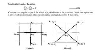
1. Solution for Laplace Equation
𝜕2𝑢
𝜕𝑥2 +
𝜕2𝑢
𝜕𝑦2 = 0 ----------(12)
Consider a rectangular region 𝑅 for which 𝑢(𝑥, 𝑦) is known at the boundary. Divide this region into
a network of square mesh of side ℎ (assuming that an exact division of 𝑅 is possible.
Figure-2. Figure-3.

2. Replacing the derivatives in (12) by their difference approximations, we have
1
ℎ2
𝑢𝑖+1,𝑗 − 2𝑢𝑖,𝑗 + 𝑢𝑖−1,𝑗 +
1
ℎ2
𝑢𝑖,𝑗+1 − 2𝑢𝑖,𝑗 + 𝑢𝑖,𝑗−1 = 0
Or 𝑢𝑖,𝑗 =
1
4
𝑢𝑖+1,𝑗 + 𝑢𝑖−1,𝑗 + 𝑢𝑖,𝑗+1 + 𝑢𝑖,𝑗−1 ----------(13)
This shows that the value of 𝑢 at any interior mesh point is the average of its values at four
neighboring points to the left, right, above and below. Equation (13) is called standard 5-point
formula as shown in figure-2.

3. Sometimes a formula similar to this is used which is given by,
𝑢𝑖,𝑗 =
1
4
(𝑢𝑖−1,𝑗+1 + 𝑢𝑖+1,𝑗−1 + 𝑢𝑖+1,𝑗+1 + 𝑢𝑖−1,𝑗−1) ----------(14)
Which shows that the value of 𝑢 at any interior mesh point is the average of its values at four
neighboring diagonal mesh points. Equation (14) is also called the diagonal 5-point formula as
shown in figure-3. Although this is less accurate than the standard 5-point formula, it is used in
getting a good approximation for the starting values at the mesh points.

4. By applying 5-point formula at each interior mesh point, we arrive at linear equations in the nodal
values 𝑢𝑖,𝑗. These equations can be solved by Jacobi’s iterative method or Gauss-Seidal iterative
method. The iterative methods are repeated till the difference between two consecutive iterates become
negligible.
1. Jacobi’s method: Denoting the 𝑛𝑡ℎ iterative value of 𝑢𝑖,𝑗 by 𝑢𝑖,𝑗
𝑛
, the iterative formula to solve is,
𝑢𝑖,𝑗
(𝑛+1)
=
1
4
𝑢𝑖+1,𝑗
(𝑛)
+ 𝑢𝑖−1,𝑗
(𝑛)
+ 𝑢𝑖,𝑗+1
(𝑛)
+ 𝑢𝑖,𝑗−1
(𝑛)
----------(15)
It gives improved values of 𝑢𝑖,𝑗 at the interior mesh points.
1. Gauss-Seidal method or Leibmann’s method: In this method, the iteration formula is,
𝑢𝑖,𝑗
(𝑛+1)
=
1
4
𝑢𝑖+1,𝑗
(𝑛)
+ 𝑢𝑖−1,𝑗
(𝑛+1)
+ 𝑢𝑖,𝑗+1
(𝑛+1)
+ 𝑢𝑖,𝑗−1
(𝑛)
----------(16)
This utilizes the latest iterative values available and evaluates the mesh points symmetrically from
left to right along successive rows.

5. Note:
 The accuracy of the calculations depends on the mesh-size i.e. smaller the 𝒉, better the
accuracy. But if 𝒉 is too small, it increases the computations.
 The error in solving Laplace and Poisson’s equations by finite-difference method is of the
order 𝒐 𝒉𝟐 .

6. Solution: Solution is symmetric about principal
diagonal as shown in figure. Using 5-point formula at
each of the unknown mesh points, we have,
4𝑎 = 𝑏 + 𝑑 + 2
4𝑏 = 2𝑎 + 4
4𝑑 = 2𝑎
Solving for unknowns,
𝑎 = 𝑐 = 1; 𝑏 = 1.5; 𝑑 = 0.5
Solved examples:
1. Solve
𝝏𝟐𝒖
𝝏𝒙𝟐 +
𝝏𝟐𝒖
𝝏𝒚𝟐 = 𝟎, with 𝒉 =
𝟏
𝟑
, 𝒖 𝒙, 𝟏 = 𝒖 𝟎, 𝒚 = 𝟎, 𝟎 < 𝒙, 𝒚 < 𝟏 and also 𝒖 𝒙, 𝟎 = 𝟗 𝒙 − 𝒙𝟐
,
𝒖 𝟏, 𝒚 = 𝟗 𝒚 − 𝒚𝟐 .

7. 2. Solve
𝝏𝟐𝒖
𝝏𝒙𝟐 +
𝝏𝟐𝒖
𝝏𝒚𝟐 = 𝟎, with 𝒉 =
𝟏
𝟒
, 𝒖 𝒙, 𝟎 = 𝒖 𝒙, 𝟏 = 𝟎, 𝟎 < 𝒙, 𝒚 < 𝟏 and also 𝒖 𝟎, 𝒚 =
𝟏𝟎𝟎, 𝒖 𝟏, 𝒚 = 𝟎 using Leibmann’s method.
Solution: With reference to the figure, we have equations
in 6 unknowns.
4𝑎 = 100 + 𝑏 + 𝑑
4𝑏 = 𝑎 + 𝑒 + 𝑐
4𝑐 = 𝑏 + 𝑓
4𝑑 = 100 + 2𝑎 + 𝑒
4𝑒 = 2𝑏 + 𝑑 + 𝑓
4𝑓 = 2𝑐 + 𝑒
Solving using Leibmann’s method or Gauss seidal
method(3 iterations),
𝑎 𝑏 𝑐 𝑑 𝑒 𝑓
0 0 0 0 0 0
25 6.25 1.5625 37.5 12.5 0.78125
35.9375 12.5 3.3203 46.09375 17.96875 6.1523 and so on.

8. Exercise problems:
1. Solve Laplace equation 𝛁𝟐
𝒖 = 𝟎, 𝟎 < 𝒙, 𝒚 < 𝟐, with 𝒉 =
𝟏
𝟐
, 𝒖 𝒙, 𝟎 = 𝟎, 𝒖 𝒙, 𝟐 = 𝟔,
𝒖 𝟎, 𝒚 = 𝟏, 𝒖 𝟐, 𝒚 = 𝟏.
2. Solve 𝛁𝟐𝒖 = 𝟎, 𝒙 < 𝟏, 𝒚 < 𝟏, 𝒉 =
𝟏
𝟐
. Also, 𝒖 ±𝟏, 𝒚 = 𝒚𝟐, 𝒖 𝒙, ±𝟏 = 𝒙𝟐.
3. Solve 𝛁𝟐
𝒖 = 𝟎, 𝟎 < 𝒙, 𝒚 < 𝟒, with 𝒉 = 𝟏,𝒖 𝒙, 𝟎 = 𝒙𝟐
+ 𝟐𝒙, 𝒖 𝟎, 𝒚 = −𝟐𝒚 − 𝒚𝟐
, 𝒖 𝟒, 𝒚 =
𝟐𝟒 − 𝒚𝟐 − 𝟐𝒚, 𝒖 𝒙, 𝟒 = 𝒙𝟐 + 𝟐𝒙 − 𝟐𝟒.
(Hint: Negative symmetry to be considered. Number of variables reduces to six.)

9. Poisson Equation
The Poisson equation is an elliptic partial differential equation that frequently
emerges when modeling electromagnetic systems. However, like many other partial
differential equations, exact solutions are difficult to obtain for complex
geometries. This motivates the use of numerical methods in order to provide
accurate results for real-world systems. One very simple algorithm is the Finite-
Difference Method (FDM), which works by replacing the continuous derivative
operators with approximate finite differences. Although the Finite-Difference
Method is one of the oldest methods ever devised, comprehensive information is
difficult to find compiled in a single reference.

10. • Poisson differential equation is
𝜕2𝑢
𝜕𝑥2 +
𝜕2𝑢
𝜕𝑦2 = 𝑓 𝑥, 𝑦 ---------- (1)
• Its method of solution is similar to that of Laplace equation. Here the
standard 5-point formula takes the form,
𝑢𝑖−1,𝑗 + 𝑢𝑖+1,𝑗 + 𝑢𝑖,𝑗+1 + 𝑢𝑖,𝑗−1 − 4𝑢𝑖,𝑗 = ℎ2𝑓(𝑖ℎ, 𝑗ℎ) ---------- (2)
By applying formula (2) at each interior mesh point, we arrive at linear
equations in the nodal values 𝑢𝑖,𝑗. These equations can be solved by
Gauss-Seidal iterative method. The iterative methods are repeated till the
difference between two consecutive iterates become negligible.

11. Examples:
1) With 𝒉 = 𝟏, solve
𝝏𝟐𝒖
𝝏𝒙𝟐 +
𝝏𝟐𝒖
𝝏𝒚𝟐 = −𝟏𝟎 𝒙𝟐
+ 𝒚𝟐
+ 𝟏𝟎 , 𝟎 < 𝒙, 𝒚 < 𝟑 and
𝒖 = 𝟎 on the boundary.
Solution: x 0 1 2 3
y 0 1 2 3
By five point formula,
𝑢1 =
1
4
𝑢2 + 𝑢3 + 150 −−−− − 1
𝑢2 =
1
4
𝑢1 + 𝑢4 + 180 −−−− −(2)
𝑢3=
1
4
𝑢1 + 𝑢4 + 120 −−−− − 3
𝑢4 =
1
4
𝑢2 + 𝑢3 + 150 −−−− −(4)

12. From equation (1) and (4), 𝑢1 = 𝑢4.
Hence equations becomes
4𝑢1 − 𝑢2 − 𝑢3 = 150, 4𝑢2 − 2𝑢1 = 180, 4𝑢3 − 2𝑢1 = 120.
By solving these equations we get,
𝑢1 = 𝑢4 = 75, 𝑢2 = 82.5, 𝑢3 = 67.5.

13. 2) Solve 𝛁𝟐𝒖 = −𝟖𝟏𝒙𝒚, 𝟎 < 𝒙, 𝒚 < 𝟏, 𝒉 =
𝟏
𝟑
. Also, 𝒖 𝟎, 𝒚 = 𝒖 𝒙, 𝟎 = 𝟎,
𝒖 𝟏, 𝒚 = 𝒖 𝒙, 𝟏 = 𝟏𝟎𝟎.
Solution:
x 0 1/3 2/3 1
y 0 1/3 2/3 1
By standard five point formula,
𝑢1 =
1
4
𝑢2 + 𝑢3 + 102 −−−− −(1)
𝑢2 =
1
4
𝑢1 + 𝑢4 + 204 −−−− −(2)
𝑢3=
1
4
𝑢1 + 𝑢4 + 1 −−−− − 3
𝑢4 =
1
4
𝑢2 + 𝑢3 + 102 −−−− −(4)

14. From equation (1) and (4), 𝑢1 = 𝑢4.
Hence equations are:
4𝑢1 − 𝑢2 − 𝑢3 = 102, 2𝑢1 − 4𝑢2 = −204, 2𝑢1 − 4𝑢3 = −1
Solving theses equations, we get 𝑢1 = 𝑢4 = 51, 𝑢2 = 76, 𝑢3 = 26.
• Exercise problems:
1) Solve 𝛻2𝑢 = −1, 𝑥 < 2, 𝑦 < 2, ℎ = 1.
Also, 𝑢 −2, 𝑦 = 𝑢 𝑥, 2 =𝑢 2, 𝑦 = 𝑢 𝑥, −2 = 0.
2) Solve 𝛻2𝑢 = −1, 𝑥 < 2, 𝑦 < 2, ℎ = 1.
Also, 𝑢 −2, 𝑦 = 𝑢 𝑥, 2 =𝑢 2, 𝑦 = 𝑢 𝑥, −2 = 0.
3) Solve 𝛻2𝑢 = −1, 𝑥 < 1, 𝑦 < 1, ℎ =
1
2
. Also, 𝑢 ±1, 𝑦 = 𝑢 𝑥, ±1 = 0.