The EM algorithm is an iterative method to find maximum likelihood estimates of parameters in probabilistic models with latent variables. It has two steps: E-step, where expectations of the latent variables are computed based on current estimates, and M-step, where parameters are re-estimated to maximize the expected complete-data log-likelihood found in the E-step. As an example, the EM algorithm is applied to estimate the parameters of a Gaussian mixture model, where the latent variables indicate component membership of each data point.

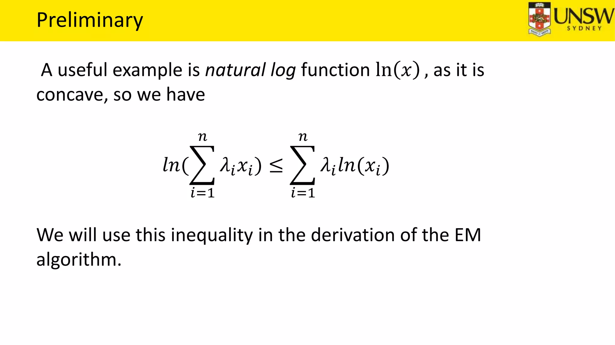
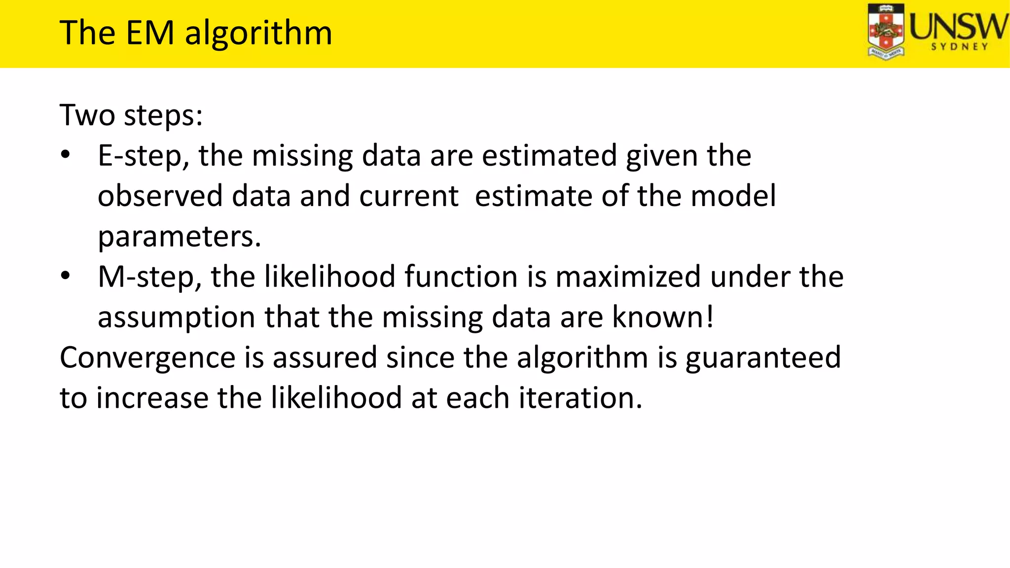
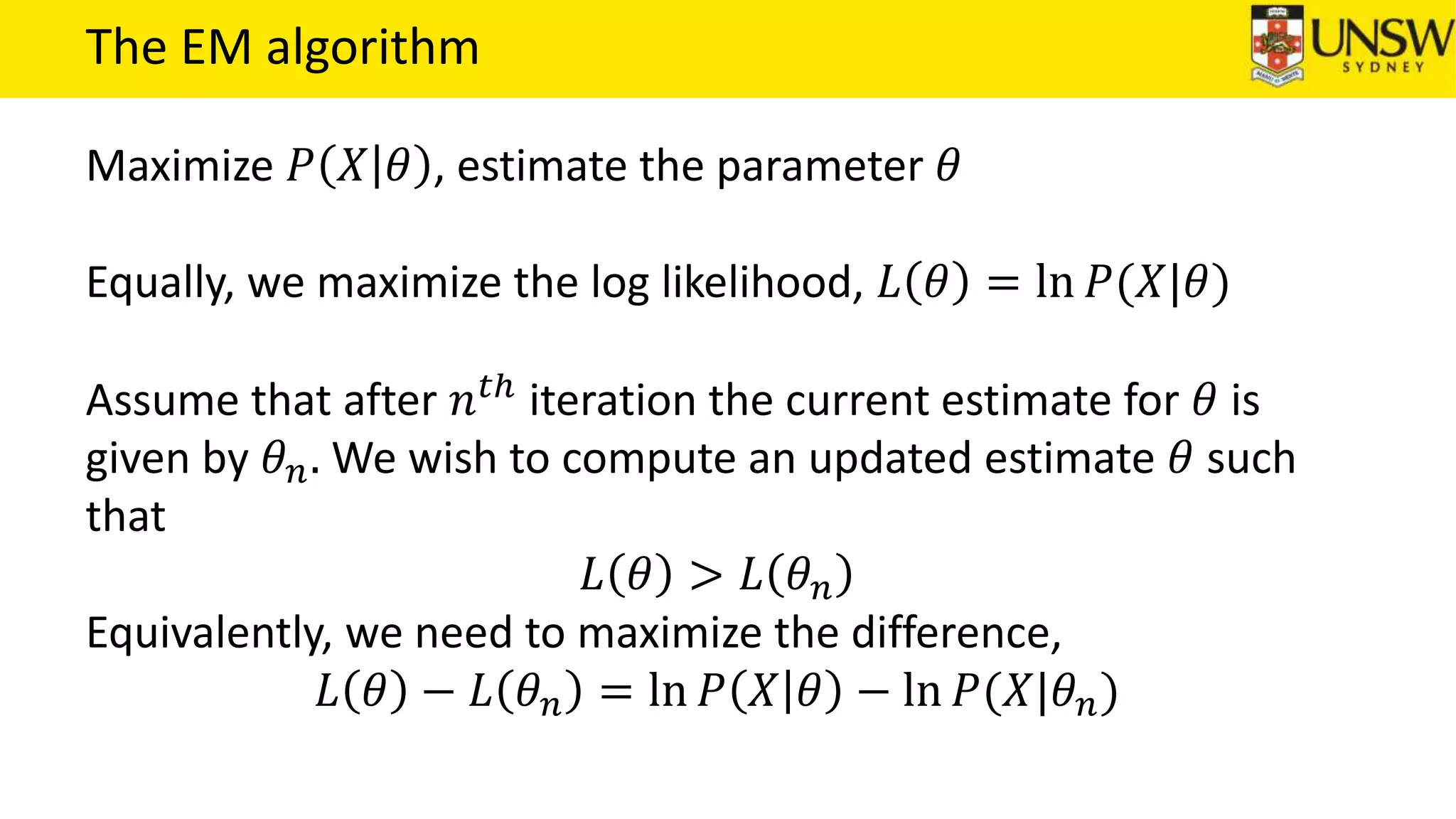
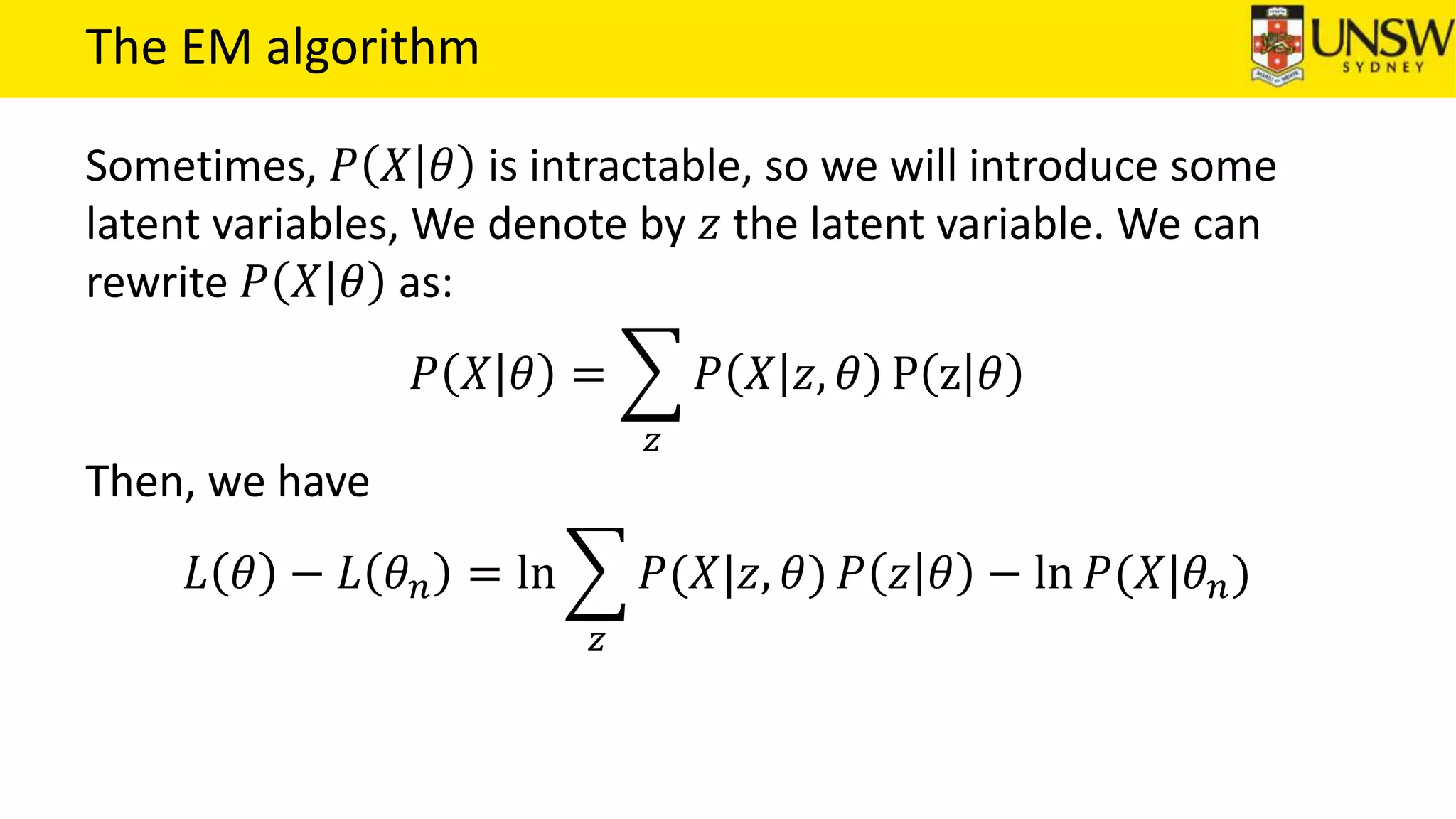
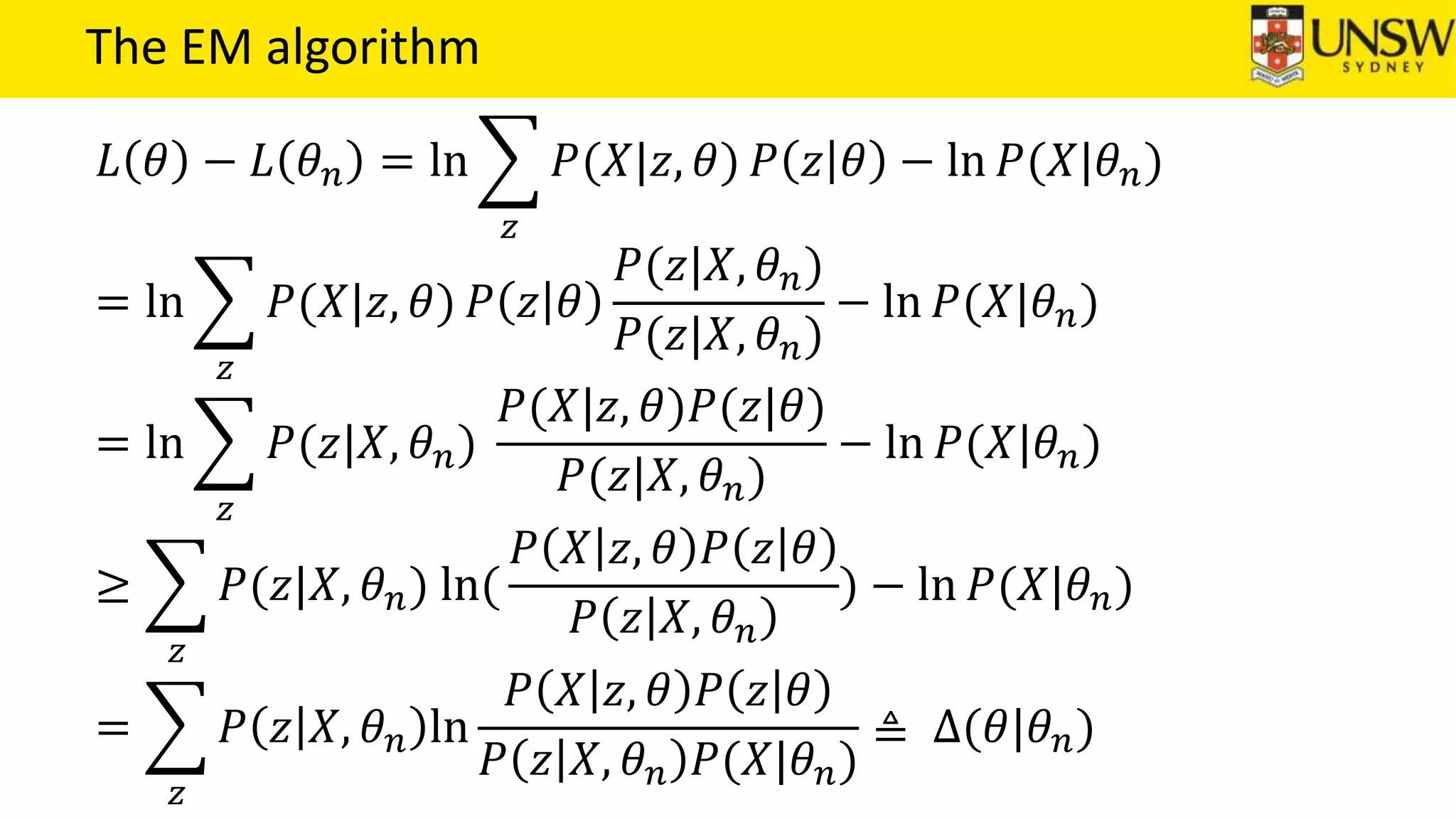
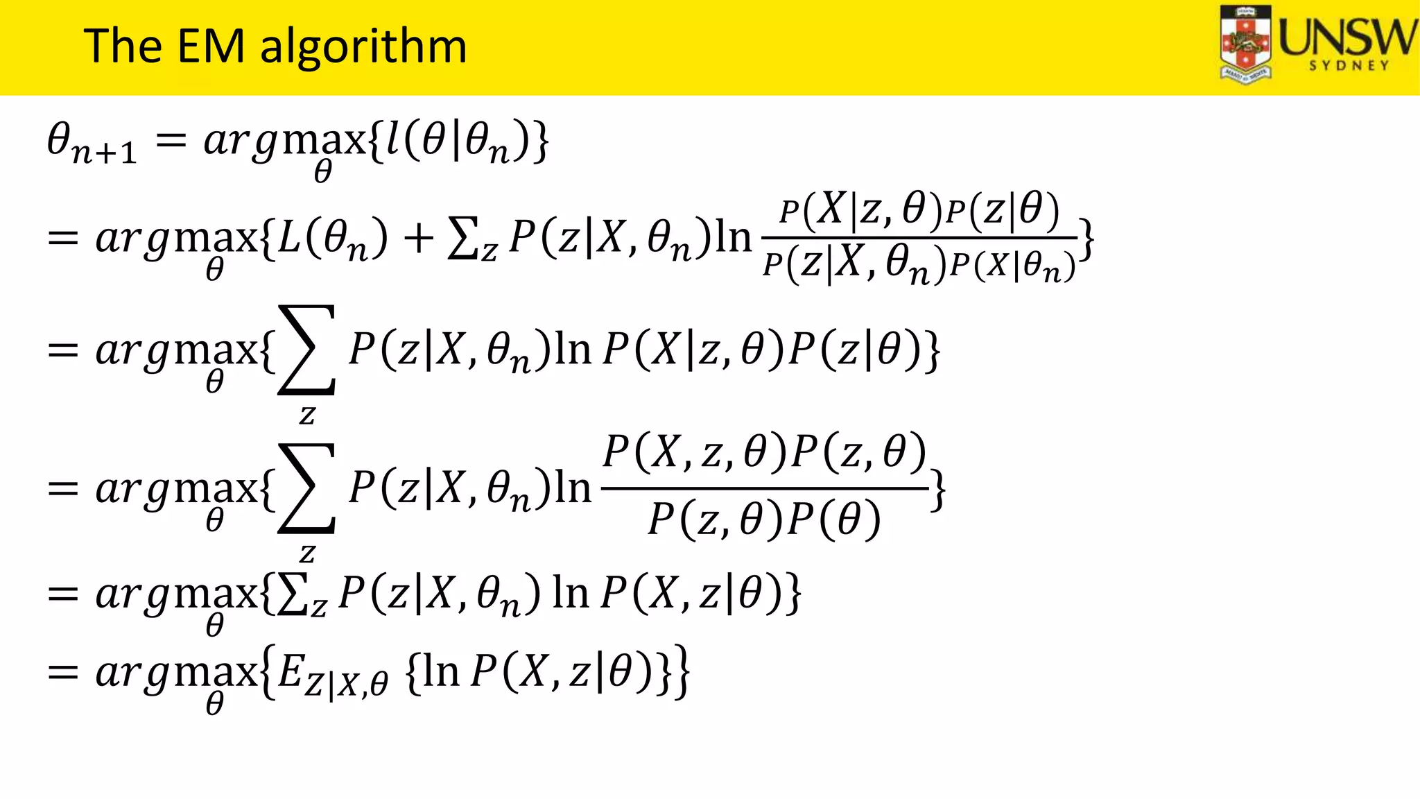
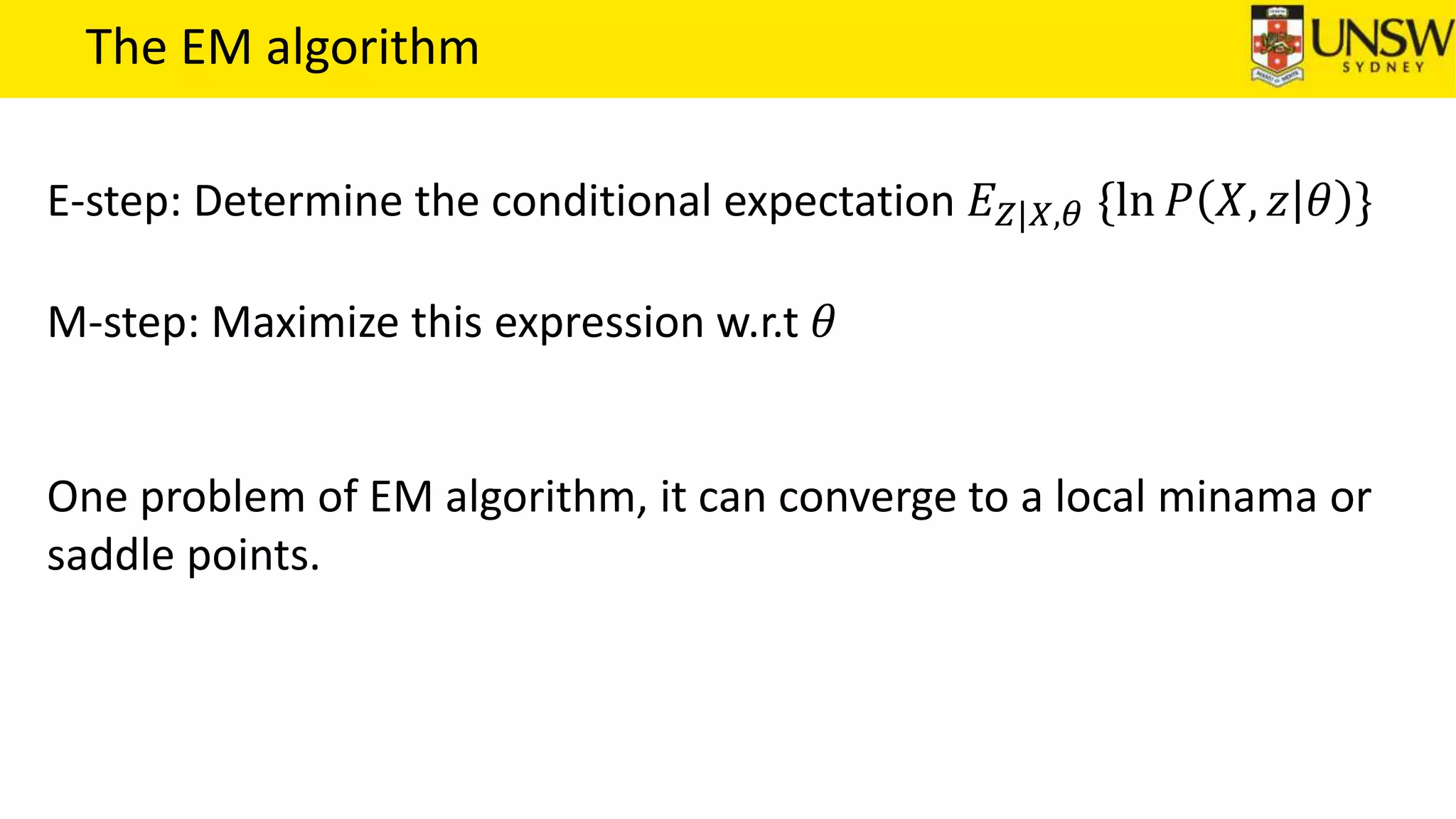
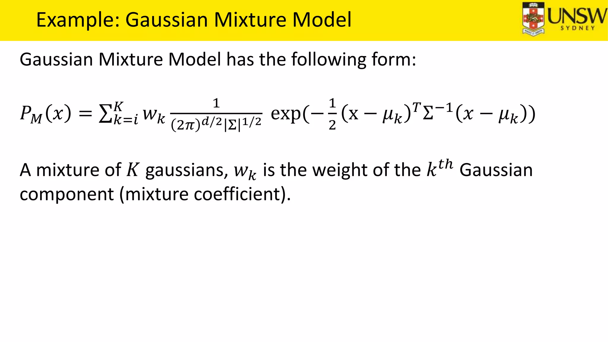
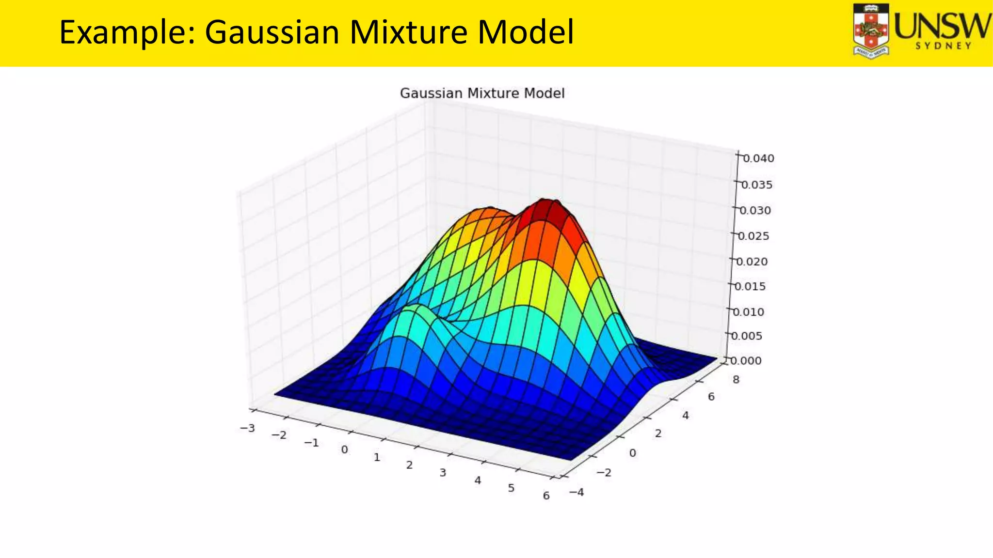
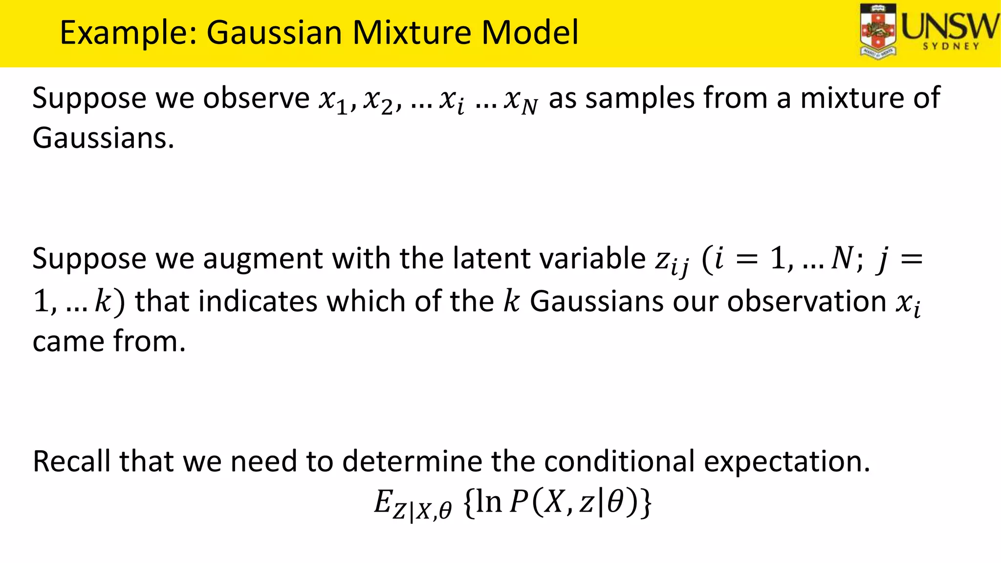
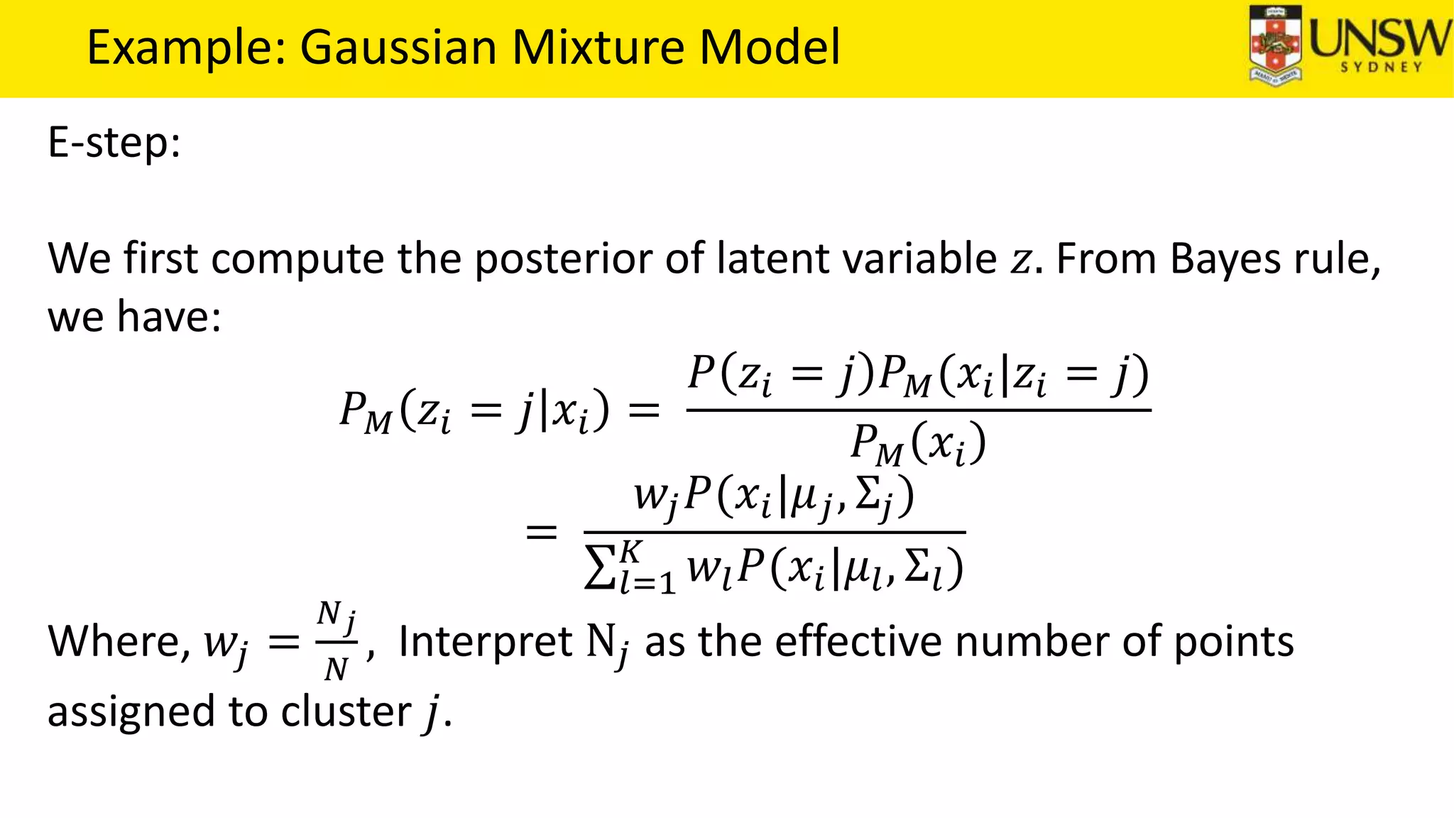
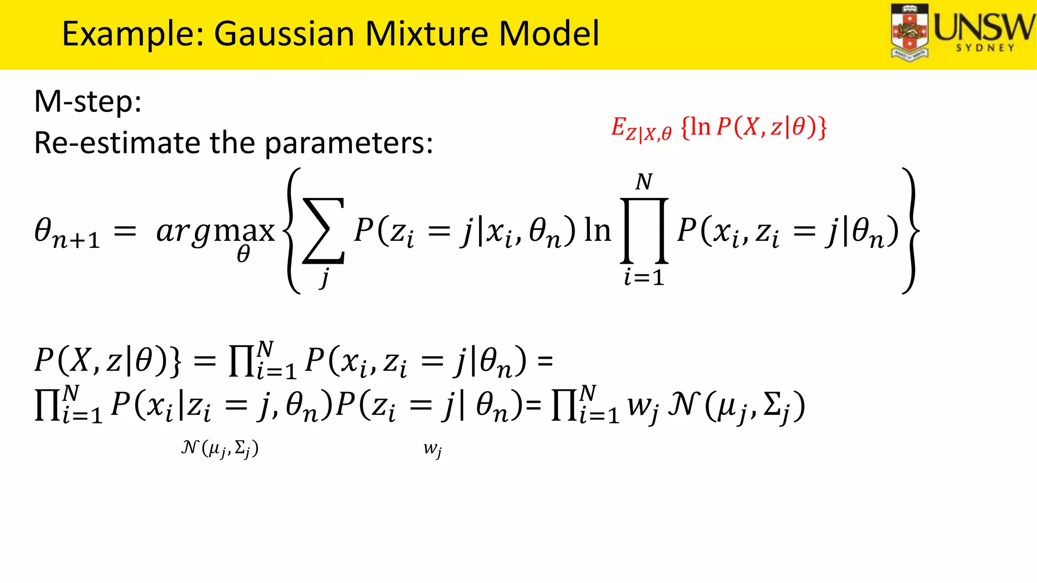
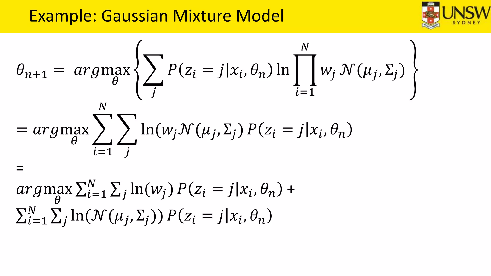
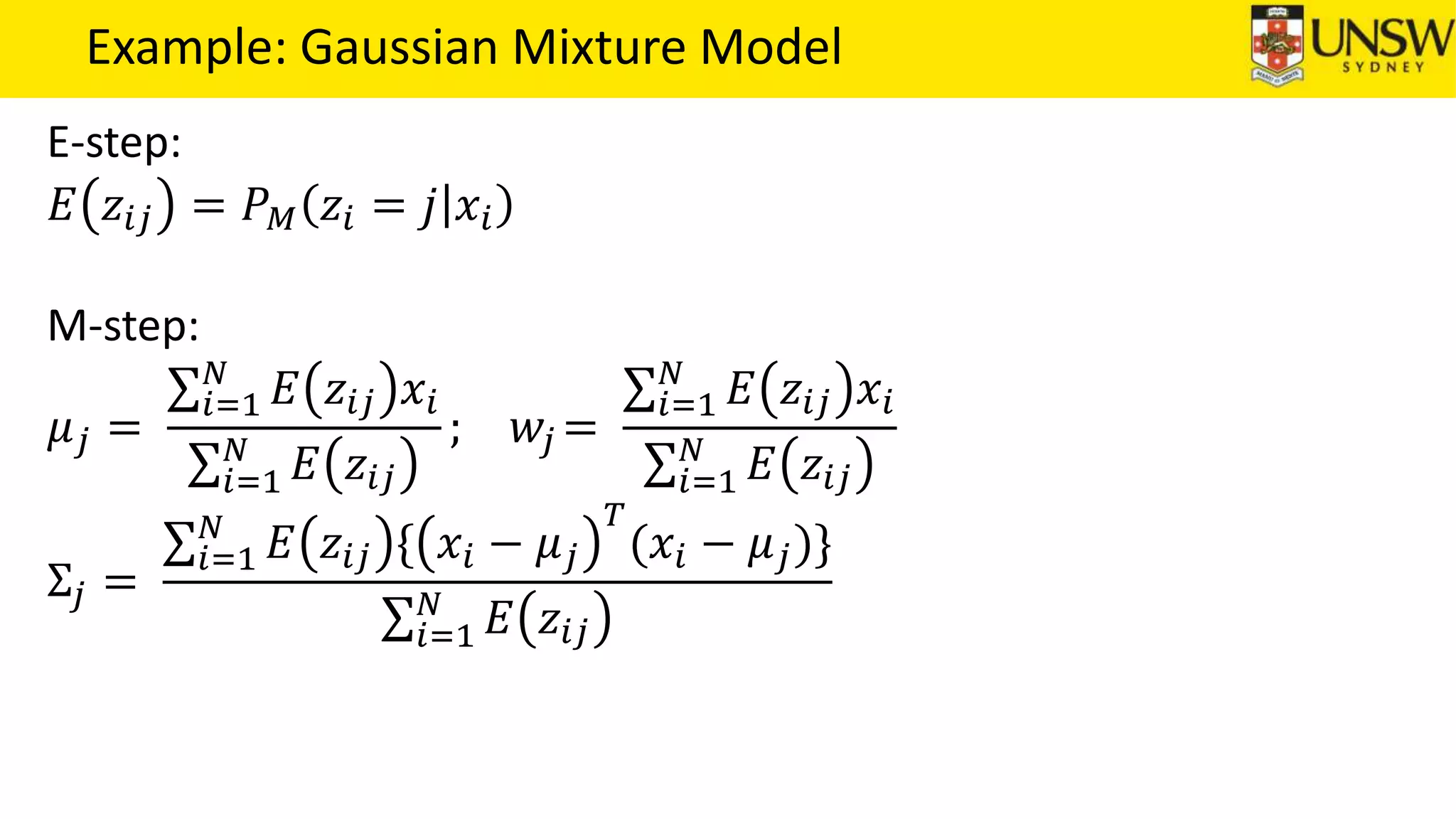
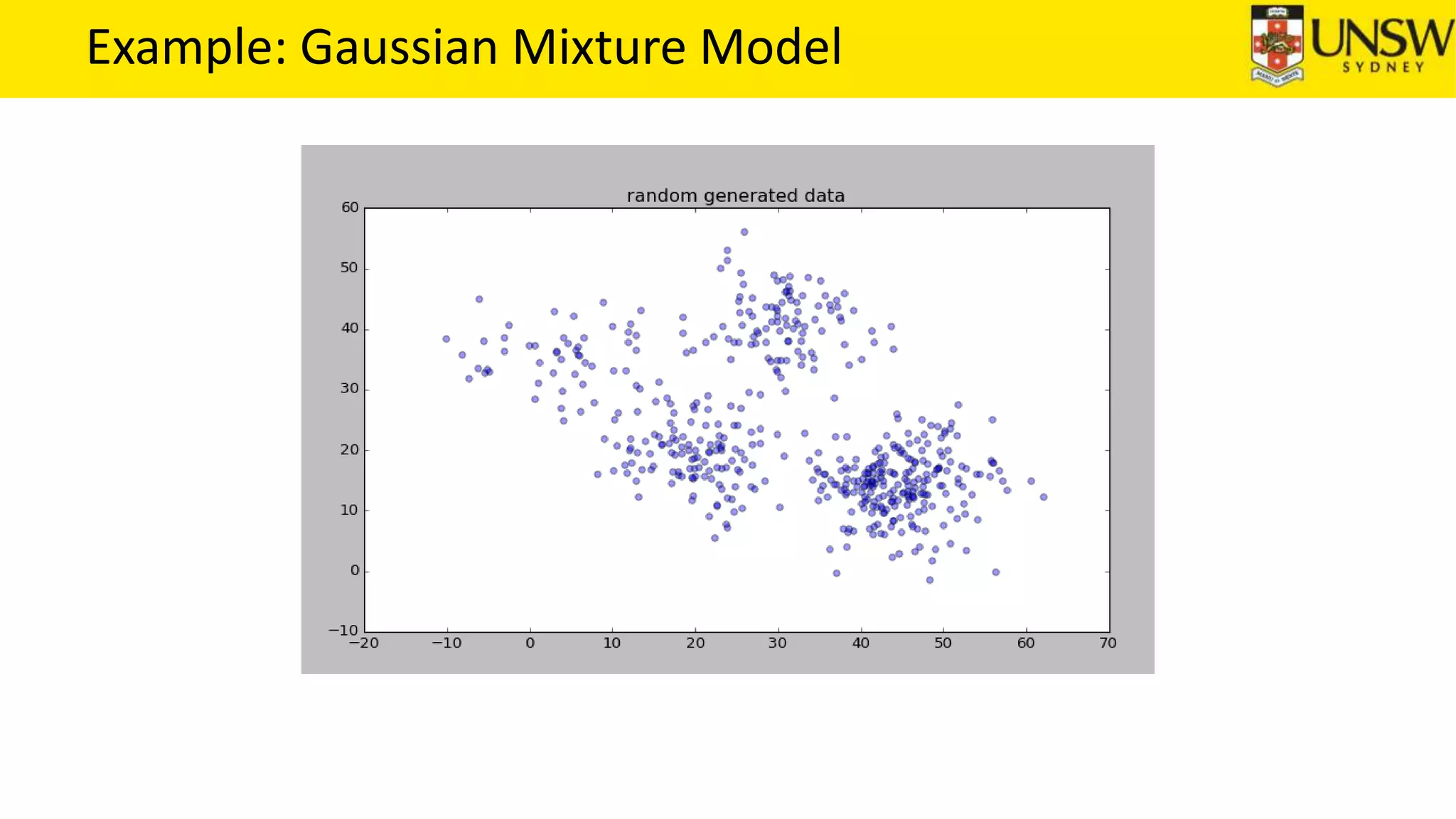
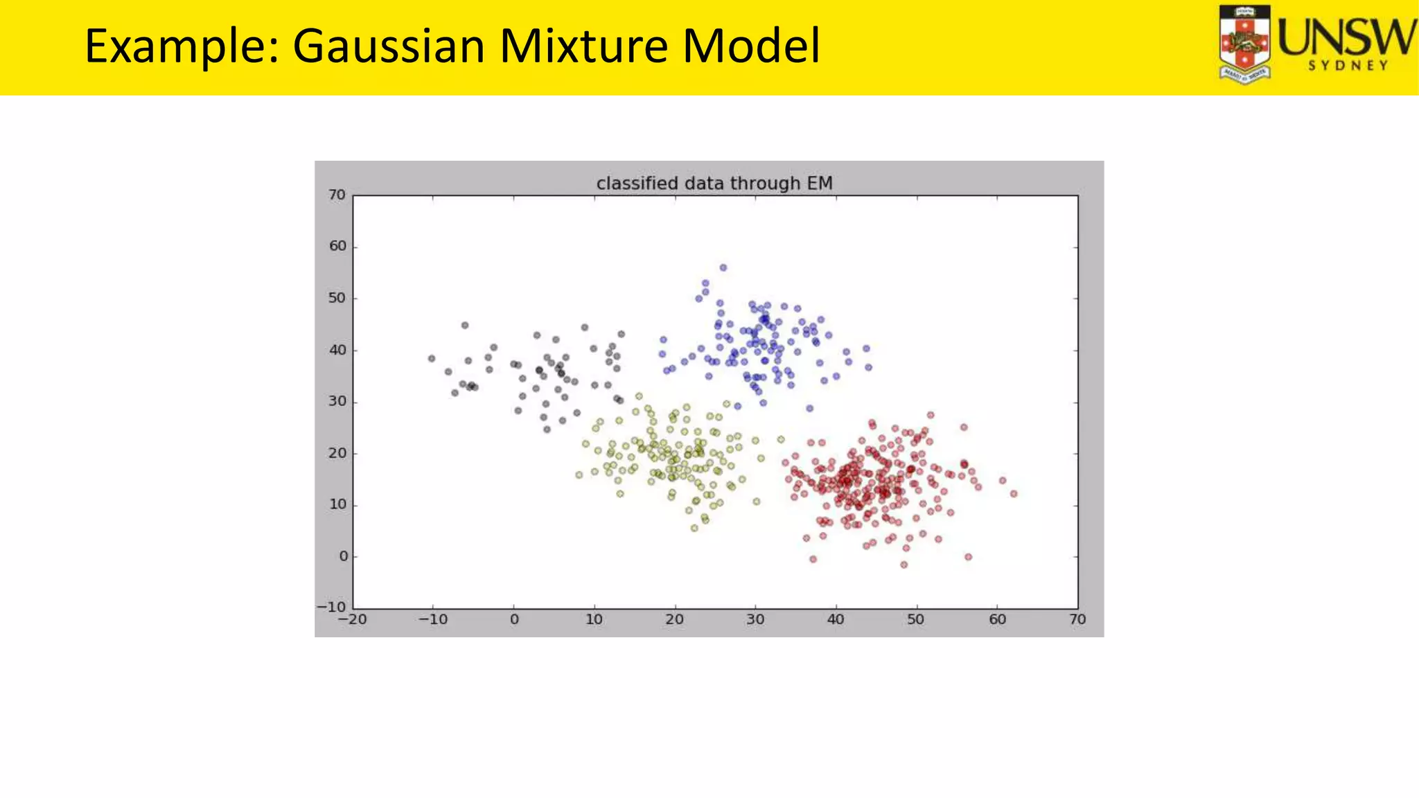
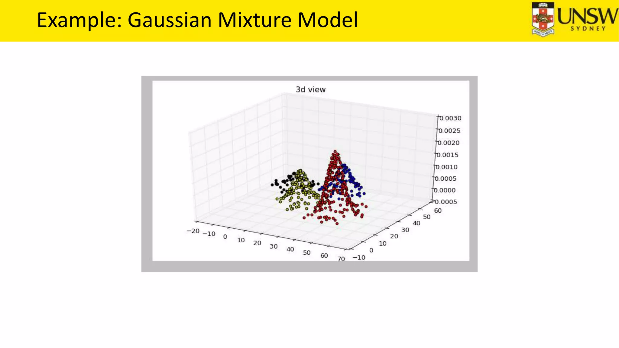
1. The Expectation Maximization
Algorithm
Presenter: Shuai Zhang, CSE, UNSW

2. Content
• Introduction
• Preliminary
• EM-Algorithm
• Example: Gaussian Mixture Model

3. Introduction
EM, is one of the top 10 data mining algorithms
The other nine are: C4.5, k-means, SVM, Apriori,
PageRank, AdaBoost, kNN, Naïve Bayes, and CART
It is a popular tool in statistical estimation problems
involving incomplete data, and mixture estimation .
The EM algorithm is an efficient iterative procedure to
compute the maximum likelihood (ML) estimate in the
presence of missing or hidden data.

4. Preliminary
Definition 1: Let 𝑓 be a real valued function defined on
an interval I ∈ 𝑎, 𝑏 , 𝑓 is said to be convex on 𝐼 if
∀𝑥1, 𝑥2 ∈ 𝐼, 𝜆 ∈ 0,1 ,
𝑓 𝜆𝑥1 + 1 − 𝜆 𝑥2 ≤ 𝜆𝑓 𝑥1 + 1 − 𝜆 𝑓 𝑥2
𝑓 is said to be strictly convex if the inequality is strict.

5. Preliminary
Intuitively, this definition
states that the function
falls below or is never
above the straight line
from points (𝑥1, 𝑓 𝑥1 to
(𝑥2, 𝑓 𝑥2

6. Preliminary
Definition 2: 𝑓 is concave if −𝑓 is convex
Definition 3: If 𝑓 x is twice differentiable on 𝑎, 𝑏 and
𝑓′′
𝑥 ≥ 0 on 𝑎, 𝑏 then 𝑓(𝑥) is convex on 𝑎, 𝑏 .

7. Preliminary
Definition 4: Jensen’s inequality, Let 𝑓 be a convex
function defined on an interval 𝐼. If 𝑥1, 𝑥2, … , 𝑥 𝑛 ∈
𝐼 𝑎𝑛𝑑 𝜆1, 𝜆2, … , 𝜆 𝑛 ≥ 0 𝑤𝑖𝑡ℎ 𝑖=1
𝑛
𝜆𝑖 = 1,
𝑓(
𝑖=1
𝑛
𝜆𝑖 𝑥𝑖) ≤
𝑖=1
𝑛
𝜆𝑖 𝑓(𝑥𝑖)
Proof: For 𝑛 = 1, this is trivial
For 𝑛 = 2, this corresponds to the definition of
convexity.
TBC…
Induction

8. Preliminary
Assume the theorem is true for some 𝑛 then, we need to
proof for 𝑛 + 1 this equation still holds.
We have 𝑖=1
𝑛+1
𝜆𝑖 = 1, this is important!
𝑓(
𝑖=1
𝑛+1
𝜆𝑖 𝑥𝑖) = 𝑓(𝜆 𝑛+1 𝑥 𝑛+1 +
𝑖=1
𝑛
𝜆𝑖 𝑥𝑖)
= 𝑓(𝜆 𝑛+1 𝑥 𝑛+1 + 1 − 𝜆 𝑛+1
1
1−𝜆 𝑛+1
𝑖=1
𝑛
𝜆𝑖 𝑥𝑖)
≤ 𝜆 𝑛+1 𝑓 𝑥 𝑛+1 + 1 − 𝜆 𝑛+1 𝑓(
1
1−𝜆 𝑛+1
𝑖=1
𝑛
𝜆𝑖 𝑥𝑖)
= 𝜆 𝑛+1 𝑓 𝑥 𝑛+1 + 1 − 𝜆 𝑛+1 𝑓( 𝑖=1
𝑛 𝜆 𝑖
1−𝜆 𝑛+1
𝑥𝑖)
TBC

9. Preliminary
≤ 𝜆 𝑛+1 𝑓 𝑥 𝑛+1 + 1 − 𝜆 𝑛+1 𝑖=1
𝑛 𝜆 𝑖
1−𝜆 𝑛+1
𝑓(𝑥𝑖)
= 𝜆 𝑛+1 𝑓 𝑥 𝑛+1 + 𝑖=1
𝑛
𝜆𝑖 𝑓(𝑥𝑖)
= 𝑖=1
𝑛+1
𝜆𝑖 𝑓(𝑥𝑖)
JE provides a simple proof that the arithmetic mean is
greater than or equal to the geometric mean.
Because
𝑖=1
𝑛 𝜆 𝑖
1−𝜆 𝑛+1
= 1,
we set 𝜆𝑖 =
𝜆 𝑖
1−𝜆 𝑛+1

10. Preliminary
A useful example is natural log function ln 𝑥 , as it is
concave, so we have
𝑙𝑛(
𝑖=1
𝑛
𝜆𝑖 𝑥𝑖) ≤
𝑖=1
𝑛
𝜆𝑖 𝑙𝑛(𝑥𝑖)
We will use this inequality in the derivation of the EM
algorithm.

11. The EM algorithm
Two steps:
• E-step, the missing data are estimated given the
observed data and current estimate of the model
parameters.
• M-step, the likelihood function is maximized under the
assumption that the missing data are known!
Convergence is assured since the algorithm is guaranteed
to increase the likelihood at each iteration.

12. The EM algorithm
Maximize 𝑃 𝑋 𝜃 , estimate the parameter 𝜃
Equally, we maximize the log likelihood, 𝐿 𝜃 = ln 𝑃(𝑋|𝜃)
Assume that after 𝑛 𝑡ℎ
iteration the current estimate for 𝜃 is
given by 𝜃 𝑛. We wish to compute an updated estimate 𝜃 such
that
𝐿 𝜃 > 𝐿 𝜃 𝑛
Equivalently, we need to maximize the difference,
𝐿 𝜃 − 𝐿 𝜃 𝑛 = ln 𝑃 𝑋 𝜃 − ln 𝑃(𝑋|𝜃 𝑛)

13. The EM algorithm
Sometimes, 𝑃 𝑋 𝜃 is intractable, so we will introduce some
latent variables, We denote by 𝑧 the latent variable. We can
rewrite 𝑃 𝑋 𝜃 as:
𝑃 𝑋 𝜃 =
𝑧
𝑃 𝑋 𝑧, 𝜃 P z 𝜃
Then, we have
𝐿 𝜃 − 𝐿 𝜃 𝑛 = ln
𝑧
𝑃(𝑋|𝑧, 𝜃) 𝑃 𝑧 𝜃 − ln 𝑃(𝑋|𝜃 𝑛)

14. The EM algorithm
𝐿 𝜃 − 𝐿 𝜃 𝑛 = ln
𝑧
𝑃(𝑋|𝑧, 𝜃) 𝑃 𝑧 𝜃 − ln 𝑃(𝑋|𝜃 𝑛)
= ln
𝑧
𝑃(𝑋|𝑧, 𝜃) 𝑃 𝑧 𝜃
𝑃(𝑧|𝑋, 𝜃 𝑛)
𝑃(𝑧|𝑋, 𝜃 𝑛)
− ln 𝑃(𝑋|𝜃 𝑛)
= ln
𝑧
𝑃(𝑧|𝑋, 𝜃 𝑛)
𝑃(𝑋|𝑧, 𝜃)𝑃(𝑧|𝜃)
𝑃(𝑧|𝑋, 𝜃 𝑛)
− ln 𝑃(𝑋|𝜃 𝑛)
≥
𝑧
𝑃(𝑧|𝑋, 𝜃 𝑛) ln(
𝑃 𝑋 𝑧, 𝜃 𝑃 𝑧 𝜃
𝑃 𝑧 𝑋, 𝜃 𝑛
) − ln 𝑃(𝑋|𝜃 𝑛)
=
𝑧
𝑃 𝑧 𝑋, 𝜃 𝑛 ln
𝑃 𝑋 𝑧, 𝜃 𝑃 𝑧 𝜃
𝑃 𝑧 𝑋, 𝜃 𝑛 𝑃(𝑋|𝜃 𝑛)
≜ ∆(𝜃|𝜃 𝑛)

15. The EM algorithm
So,
𝐿 𝜃 ≥ 𝐿 𝜃 𝑛 + ∆ 𝜃 𝜃 𝑛
For convenience, we define:
𝑙 𝜃 𝜃 𝑛 ≜ 𝐿 𝜃 + ∆ 𝜃 𝜃 𝑛
So we have,
𝐿 𝜃 ≥ 𝑙 𝜃 𝜃 𝑛

16. The EM algorithm
We also observe that,
𝑙 𝜃 𝑛 𝜃 𝑛 = 𝐿 𝜃 𝑛 + ∆ 𝜃 𝑛 𝜃 𝑛
= 𝐿 𝜃 𝑛 + 𝑧 𝑃 𝑧 𝑋, 𝜃 𝑛 ln
𝑃 𝑋 𝑧, 𝜃 𝑛 𝑃 𝑧 𝜃 𝑛
𝑃 𝑧 𝑋, 𝜃 𝑛 𝑃(𝑋|𝜃 𝑛)
= 𝐿 𝜃 𝑛 + 𝑧 𝑃 𝑧 𝑋, 𝜃 𝑛 ln
𝑃 𝑋, 𝑧 𝜃 𝑛
𝑃 𝑋, 𝑧 𝜃 𝑛
= 𝐿 𝜃 𝑛
For 𝜃 = 𝜃 𝑛, the function 𝑙 𝜃 𝜃 𝑛 and 𝐿 𝜃 are equal.

17. The EM algorithm
From the following two equations:
𝐿 𝜃 ≥ 𝑙 𝜃 𝜃 𝑛
𝑙 𝜃 𝑛 𝜃 𝑛 = 𝐿 𝜃 𝑛
Any 𝜃 which increases 𝑙 𝜃 𝜃 𝑛 will finally increase 𝐿 𝜃
The EM algorithm calls for selecting 𝜃 such that 𝑙 𝜃 𝜃 𝑛 is
maximized, we denote the update value as 𝜃 𝑛+1

18. The EM algorithm

19. The EM algorithm
𝜃 𝑛+1 = 𝑎𝑟𝑔max
𝜃
{𝑙 𝜃 𝜃 𝑛 }
= 𝑎𝑟𝑔max
𝜃
{𝐿 𝜃 𝑛 + 𝑧 𝑃 𝑧 𝑋, 𝜃 𝑛 ln
𝑃 𝑋 𝑧, 𝜃 𝑃 𝑧 𝜃
𝑃 𝑧 𝑋, 𝜃 𝑛 𝑃(𝑋|𝜃 𝑛)
}
= 𝑎𝑟𝑔max
𝜃
{
𝑧
𝑃 𝑧 𝑋, 𝜃 𝑛 ln 𝑃 𝑋 𝑧, 𝜃 𝑃 𝑧 𝜃 }
= 𝑎𝑟𝑔max
𝜃
{
𝑧
𝑃 𝑧 𝑋, 𝜃 𝑛 ln
𝑃 𝑋, 𝑧, 𝜃 𝑃 𝑧, 𝜃
𝑃 𝑧, 𝜃 𝑃 𝜃
}
= 𝑎𝑟𝑔max
𝜃
𝑧 𝑃 𝑧 𝑋, 𝜃 𝑛 ln 𝑃 𝑋, 𝑧 𝜃
= 𝑎𝑟𝑔max
𝜃
𝐸 𝑍|𝑋,𝜃 {ln 𝑃 𝑋, 𝑧 𝜃 }

20. The EM algorithm
E-step: Determine the conditional expectation 𝐸 𝑍|𝑋,𝜃 {ln 𝑃 𝑋, 𝑧 𝜃 }
M-step: Maximize this expression w.r.t 𝜃
One problem of EM algorithm, it can converge to a local minama or
saddle points.

21. Example: Gaussian Mixture Model
Gaussian Mixture Model has the following form:
𝑃 𝑀 𝑥 = 𝑘=𝑖
𝐾
𝑤 𝑘
1
2𝜋 𝑑/2 Σ 1/2 exp(−
1
2
x − 𝜇 𝑘
𝑇
Σ−1
𝑥 − 𝜇 𝑘 )
A mixture of 𝐾 gaussians, 𝑤 𝑘 is the weight of the 𝑘 𝑡ℎ
Gaussian
component (mixture coefficient).

22. Example: Gaussian Mixture Model

23. Example: Gaussian Mixture Model
Suppose we observe 𝑥1, 𝑥2, … 𝑥𝑖 … 𝑥 𝑁 as samples from a mixture of
Gaussians.
Suppose we augment with the latent variable 𝑧𝑖𝑗 (𝑖 = 1, … 𝑁; 𝑗 =
1, … 𝑘) that indicates which of the 𝑘 Gaussians our observation 𝑥𝑖
came from.
Recall that we need to determine the conditional expectation.
𝐸 𝑍|𝑋,𝜃 {ln 𝑃 𝑋, 𝑧 𝜃 }

24. Example: Gaussian Mixture Model
E-step:
We first compute the posterior of latent variable 𝑧. From Bayes rule,
we have:
𝑃 𝑀 𝑧𝑖 = 𝑗 𝑥𝑖 =
𝑃 𝑧𝑖 = 𝑗 𝑃 𝑀(𝑥𝑖|𝑧𝑖 = 𝑗)
𝑃 𝑀 𝑥𝑖
=
𝑤𝑗 𝑃(𝑥𝑖|𝜇 𝑗, Σ𝑗)
𝑙=1
𝐾
𝑤𝑙 𝑃(𝑥𝑖|𝜇𝑙, Σ𝑙)
Where, 𝑤𝑗 =
𝑁 𝑗
𝑁
, Interpret N𝑗 as the effective number of points
assigned to cluster 𝑗.

25. Example: Gaussian Mixture Model
M-step:
Re-estimate the parameters:
𝜃 𝑛+1 = 𝑎𝑟𝑔max
𝜃
𝑗
𝑃 𝑧𝑖 = 𝑗 𝑥𝑖, 𝜃 𝑛 ln
𝑖=1
𝑁
𝑃 𝑥𝑖, 𝑧𝑖 = 𝑗 𝜃 𝑛
𝑃 𝑋, 𝑧 𝜃 } = 𝑖=1
𝑁
𝑃 𝑥𝑖, 𝑧𝑖 = 𝑗 𝜃 𝑛 =
𝑖=1
𝑁
𝑃 𝑥𝑖 𝑧𝑖 = 𝑗, 𝜃 𝑛 𝑃 𝑧𝑖 = 𝑗 𝜃 𝑛 = 𝑖=1
𝑁
𝑤𝑗 𝒩(𝜇 𝑗, Σ𝑗)
𝐸 𝑍|𝑋,𝜃 {ln 𝑃 𝑋, 𝑧 𝜃 }
𝒩(𝜇 𝑗, Σ𝑗) 𝑤𝑗

26. Example: Gaussian Mixture Model
𝜃 𝑛+1 = 𝑎𝑟𝑔max
𝜃
𝑗
𝑃 𝑧𝑖 = 𝑗 𝑥𝑖, 𝜃 𝑛 ln
𝑖=1
𝑁
𝑤𝑗 𝒩(𝜇 𝑗, Σ𝑗)
= 𝑎𝑟𝑔max
𝜃
𝑖=1
𝑁
𝑗
ln(𝑤𝑗 𝒩(𝜇 𝑗, Σ𝑗) 𝑃 𝑧𝑖 = 𝑗 𝑥𝑖, 𝜃 𝑛
=
𝑎𝑟𝑔max
𝜃
𝑖=1
𝑁
𝑗 ln(𝑤𝑗) 𝑃 𝑧𝑖 = 𝑗 𝑥𝑖, 𝜃 𝑛 +
𝑖=1
𝑁
𝑗 ln(𝒩(𝜇 𝑗, Σ𝑗)) 𝑃 𝑧𝑖 = 𝑗 𝑥𝑖, 𝜃 𝑛

27. Example: Gaussian Mixture Model
E-step:
𝐸 𝑧𝑖𝑗 = 𝑃 𝑀 𝑧𝑖 = 𝑗 𝑥𝑖
M-step:
𝜇 𝑗 =
𝑖=1
𝑁
𝐸 𝑧𝑖𝑗 𝑥𝑖
𝑖=1
𝑁
𝐸 𝑧𝑖𝑗
; 𝑤𝑗 =
𝑖=1
𝑁
𝐸 𝑧𝑖𝑗 𝑥𝑖
𝑖=1
𝑁
𝐸 𝑧𝑖𝑗
Σ𝑗 =
𝑖=1
𝑁
𝐸 𝑧𝑖𝑗 { 𝑥𝑖 − 𝜇 𝑗
𝑇
(𝑥𝑖 − 𝜇 𝑗)}
𝑖=1
𝑁
𝐸 𝑧𝑖𝑗

28. Example: Gaussian Mixture Model

29. Example: Gaussian Mixture Model

30. Example: Gaussian Mixture Model

31. References
1. Wu, Xindong, et al. "Top 10 algorithms in data mining." Knowledge and information systems 14.1 (2008): 1-
37.
2. http://blog.csdn.net/u014157632/article/details/65442165
3. http://www.cse.iitm.ac.in/~vplab/courses/DVP/PDF/gmm.pdf
4. http://www-staff.it.uts.edu.au/~ydxu/ml_course/em.pdf
5. http://people.csail.mit.edu/dsontag/courses/ml12/slides/lecture21.pdf
6. https://www.cs.utah.edu/~piyush/teaching/EM_algorithm.pdf
7. Machine Learning, zhihua zhou

32. Thanks!

33. Last Week
• Implement the WRMF and Lrec under our framework with side information
• Our research goal is to investigate the efficacy of incorporating multi-faceted
side information with our framework
• There are a lot of ways to embed side information
• Do not have a sure answer yet if the side information can improve the original
model
• Deep learning for recommender systems, the magazine paper
• Prepare the learning group

34. This Week
• Adjust our model and conduct experiments
• The magazine paper
• Prepare for the slides for next week’s talk in RMIT (Mark Sanderson’s Group)