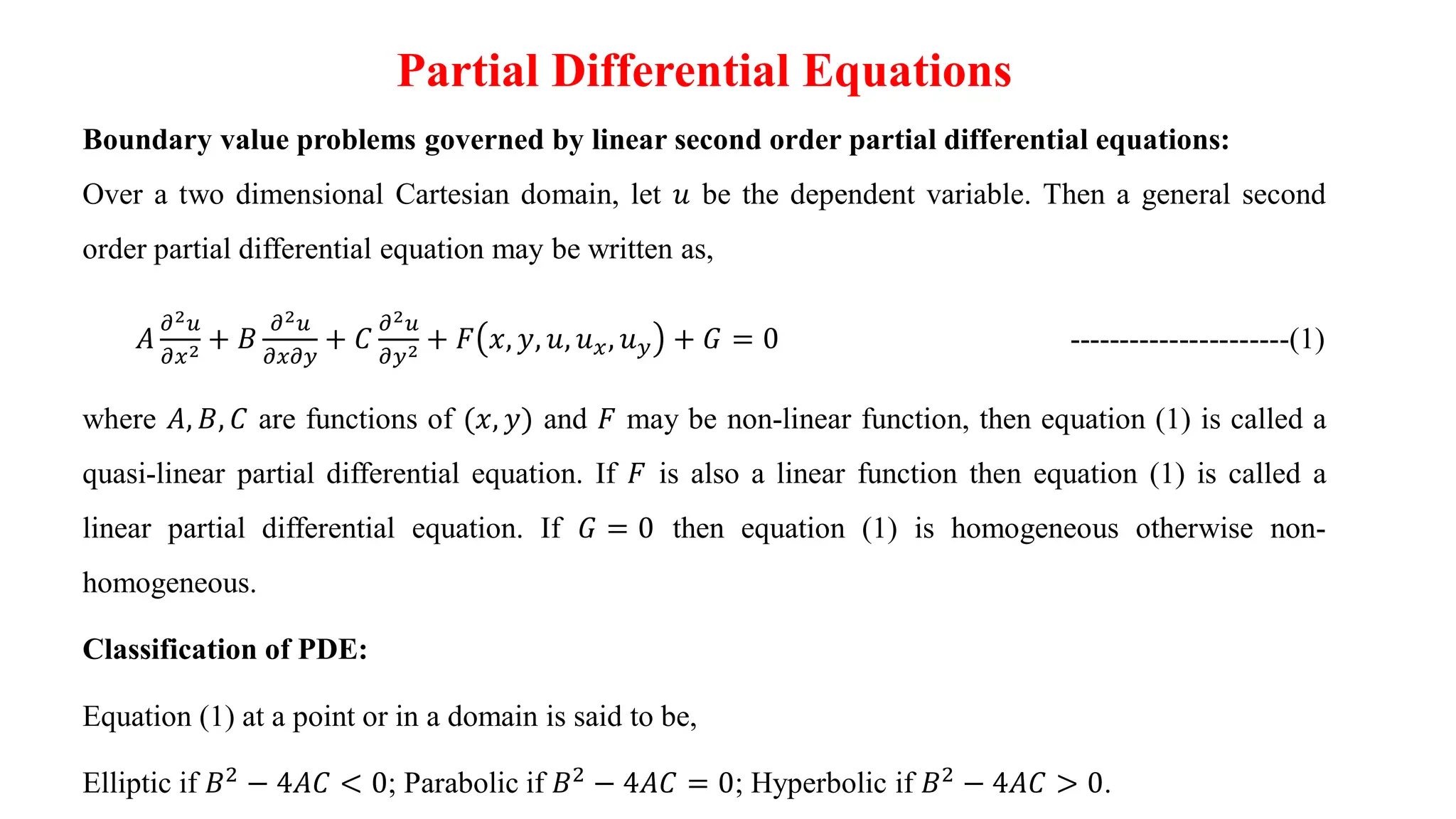
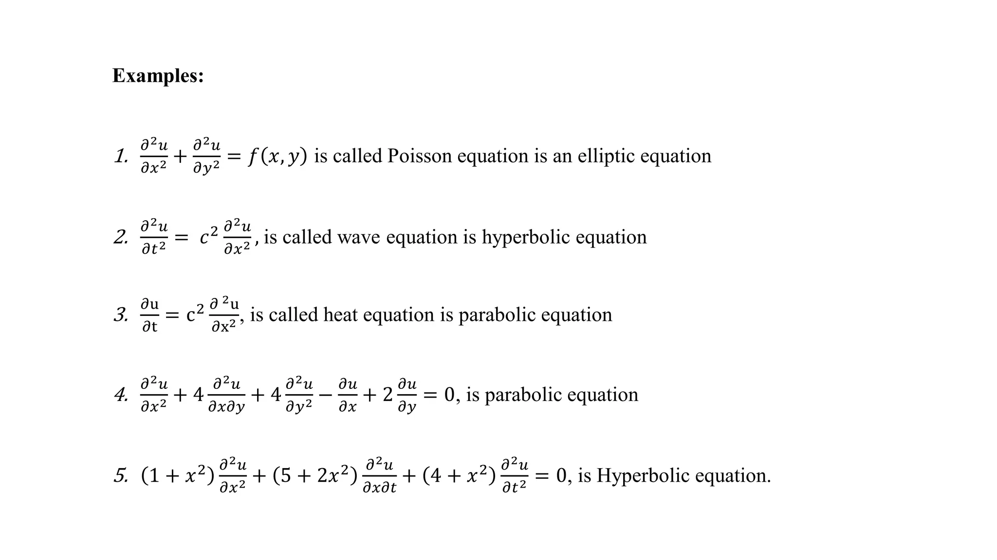
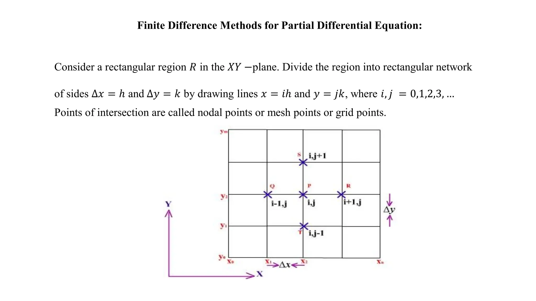
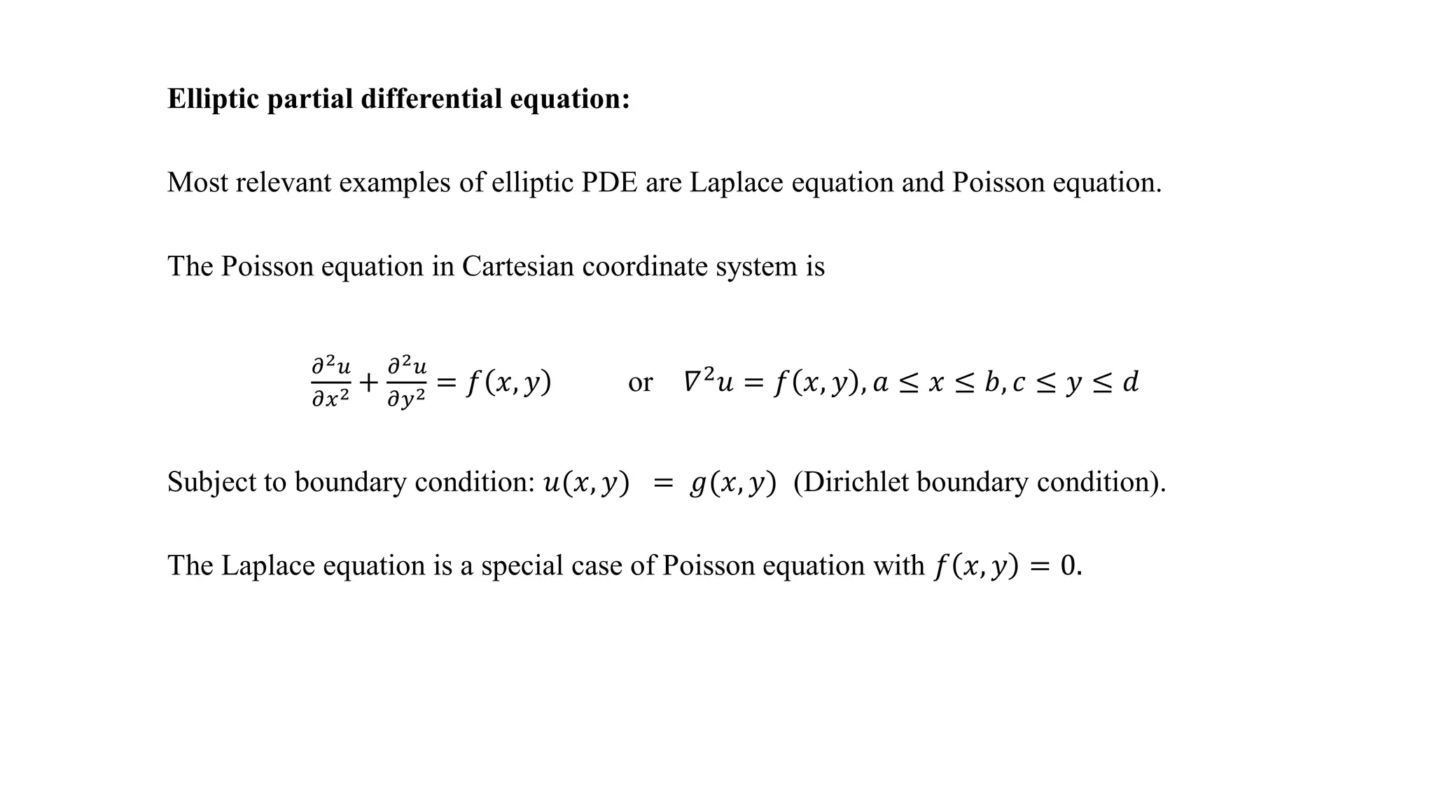
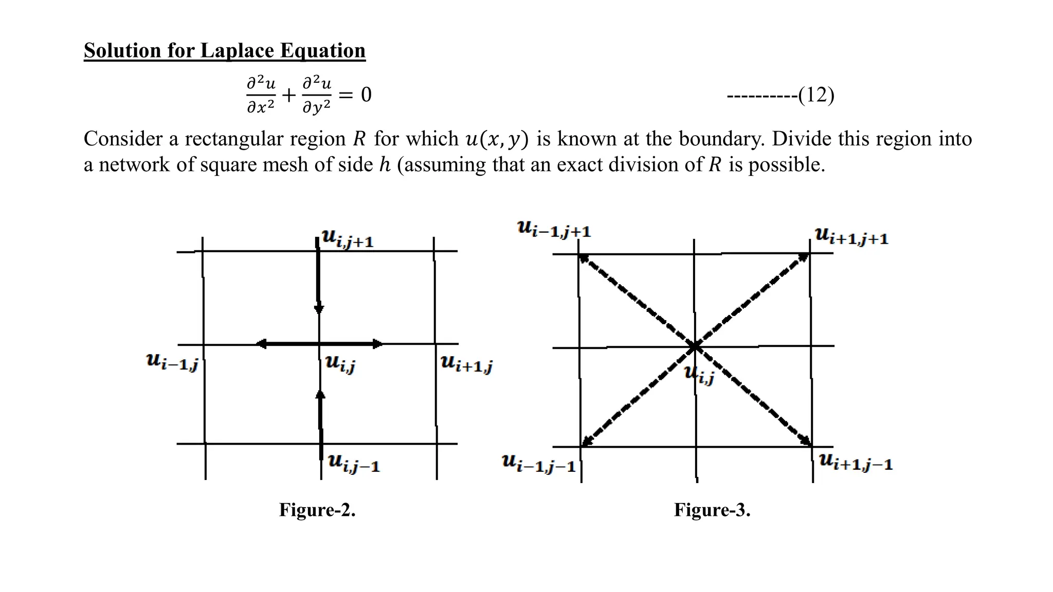
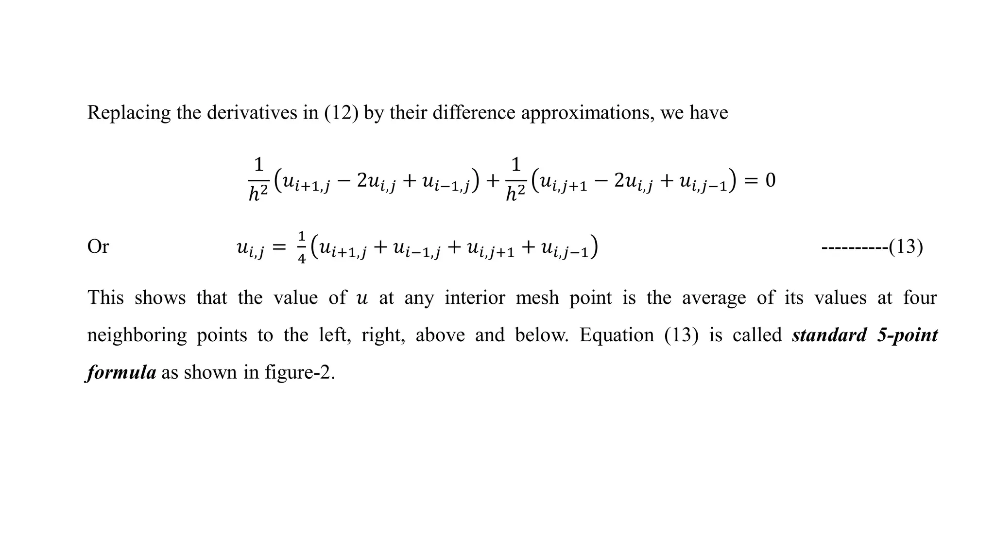
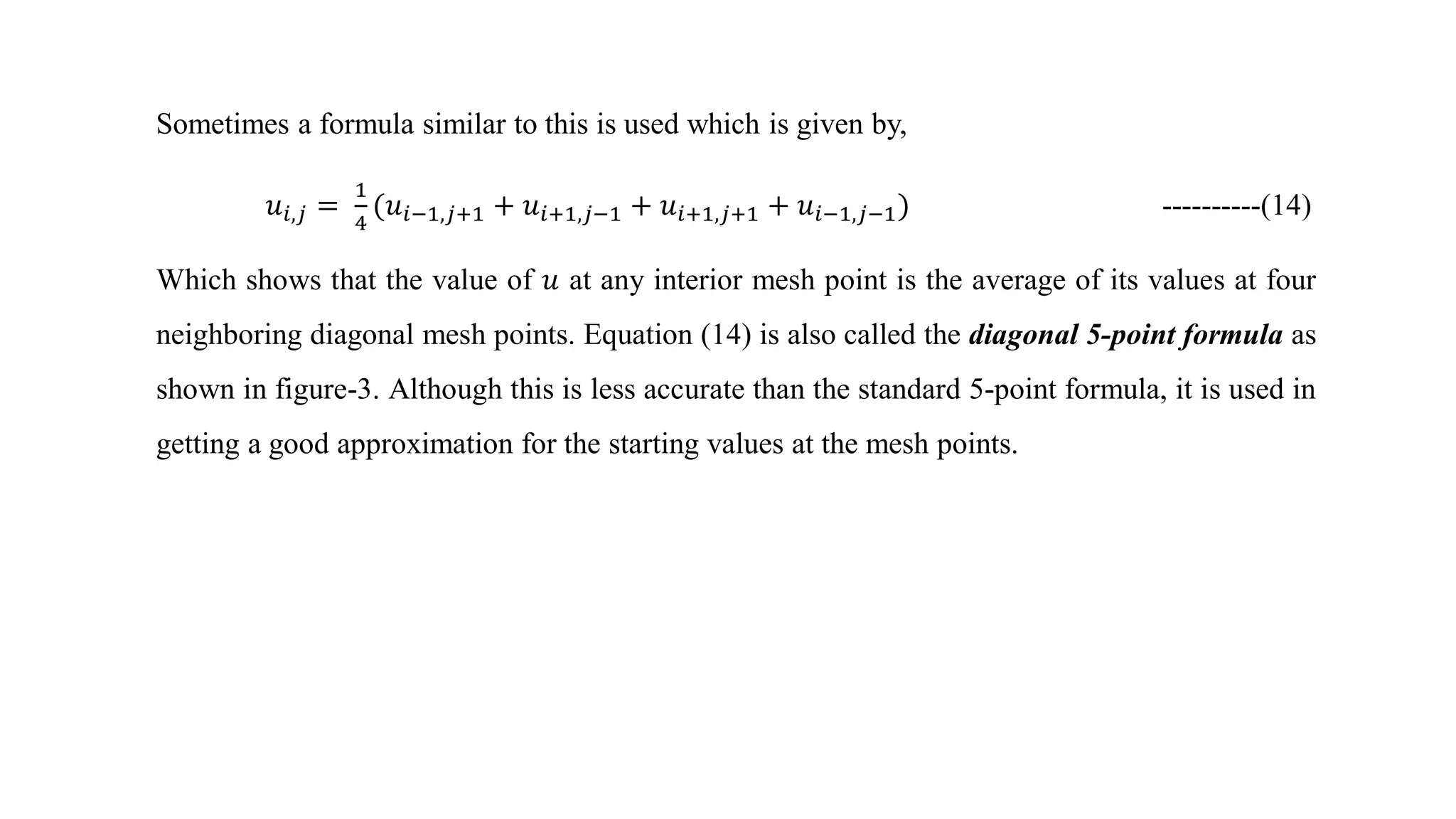
Partial Differential Equations
Boundary value problems governed by linear second order partial differential equations:
Over a two dimensional Cartesian domain, let 𝑢 be the dependent variable. Then a general second
order partial differential equation may be written as,
𝐴
𝜕2𝑢
𝜕𝑥2 + 𝐵
𝜕2𝑢
𝜕𝑥𝜕𝑦
+ 𝐶
𝜕2𝑢
𝜕𝑦2 + 𝐹 𝑥, 𝑦, 𝑢, 𝑢𝑥, 𝑢𝑦 + 𝐺 = 0 ----------------------(1)
where 𝐴, 𝐵, 𝐶 are functions of (𝑥, 𝑦) and 𝐹 may be non-linear function, then equation (1) is called a
quasi-linear partial differential equation. If 𝐹 is also a linear function then equation (1) is called a
linear partial differential equation. If 𝐺 = 0 then equation (1) is homogeneous otherwise non-
homogeneous.
Classification of PDE:
Equation (1) at a point or in a domain is said to be,
Elliptic if 𝐵2 − 4𝐴𝐶 < 0; Parabolic if 𝐵2 − 4𝐴𝐶 = 0; Hyperbolic if 𝐵2 − 4𝐴𝐶 > 0.
Examples:
1.
𝜕2𝑢
𝜕𝑥2 +
𝜕2𝑢
𝜕𝑦2 = 𝑓 𝑥, 𝑦 is called Poisson equation is an elliptic equation
2.
𝜕2𝑢
𝜕𝑡2 = 𝑐2 𝜕2𝑢
𝜕𝑥2 , is called wave equation is hyperbolic equation
3.
𝜕u
𝜕t
= c2 𝜕 2u
𝜕x2 , is called heat equation is parabolic equation
4.
𝜕2𝑢
𝜕𝑥2 + 4
𝜕2𝑢
𝜕𝑥𝜕𝑦
+ 4
𝜕2𝑢
𝜕𝑦2 −
𝜕𝑢
𝜕𝑥
+ 2
𝜕𝑢
𝜕𝑦
= 0, is parabolic equation
5. 1 + 𝑥2 𝜕2𝑢
𝜕𝑥2 + 5 + 2𝑥2 𝜕2𝑢
𝜕𝑥𝜕𝑡
+ 4 + 𝑥2 𝜕2𝑢
𝜕𝑡2 = 0, is Hyperbolic equation.
Finite Difference Methods for Partial Differential Equation:
Consider a rectangular region 𝑅 in the 𝑋𝑌 −plane. Divide the region into rectangular network
of sides Δ𝑥 = ℎ and Δ𝑦 = 𝑘 by drawing lines 𝑥 = 𝑖ℎ and 𝑦 = 𝑗𝑘, where 𝑖, 𝑗 = 0,1,2,3, …
Points of intersection are called nodal points or mesh points or grid points.
Writing 𝑢 𝑥, 𝑦 = 𝑢(𝑖ℎ, 𝑗𝑘) as simply 𝑢𝑖,𝑗, the finite difference approximations for the first order
partial derivatives can be derived using Taylor series expansion for 2 variables as follows.
We have, 𝑢 𝑥 + ℎ, 𝑦 = 𝑢𝑖+1,𝑗 = 𝑢 𝑥, 𝑦 + ℎ𝑢𝑥 𝑥, 𝑦 +
ℎ2
2!
𝑢𝑥𝑥 𝑥, 𝑦 + ⋯ -----------(2)
Thus, the forward difference formula can be written as,
𝜕𝑢
𝜕𝑥 𝑖,𝑗
=
1
ℎ
𝑢𝑖+1,𝑗 − 𝑢𝑖,𝑗 + 𝑂 ℎ -----------(3)
Similarly, 𝑢 𝑥 − ℎ, 𝑦 = 𝑢𝑖−1,𝑗 = 𝑢 𝑥, 𝑦 − ℎ𝑢𝑥 𝑥, 𝑦 +
ℎ2
2!
𝑢𝑥𝑥 𝑥, 𝑦 + ⋯ -----------(4)
Thus, the backward difference formula can be written as,
𝜕𝑢
𝜕𝑥 𝑖,𝑗
=
1
ℎ
𝑢𝑖,𝑗 − 𝑢𝑖−1,𝑗 + 𝑂 ℎ -----------(5)
The central difference formula can be obtained by Eq.(2) –Eq.(4) as,
𝜕𝑢
𝜕𝑥 𝑖,𝑗
=
1
2ℎ
𝑢𝑖+1,𝑗 − 𝑢𝑖−1,𝑗 + 𝑂 ℎ2 -----------(6)
The finite difference approximations for the second order partial derivatives can be obtained by adding
Eq.(2) and (4).
𝜕2𝑢
𝜕𝑥2
𝑖,𝑗
=
1
ℎ2 𝑢𝑖+1,𝑗 − 2𝑢𝑖,𝑗 + 𝑢𝑖−1,𝑗 + 𝑂 ℎ2 -----------(7)
Similarly,
Forward:
𝜕𝑢
𝜕𝑦 𝑖,𝑗
=
1
𝑘
𝑢𝑖,𝑗+1 − 𝑢𝑖,𝑗 + 𝑂(𝑘) -----------(8)
Backward:
𝜕𝑢
𝜕𝑦 𝑖,𝑗
=
1
𝑘
𝑢𝑖,𝑗 − 𝑢𝑖,𝑗−1 + 𝑂 𝑘 -----------(9)
Central:
𝜕𝑢
𝜕𝑦 𝑖,𝑗
=
1
2𝑘
𝑢𝑖,𝑗+1 − 𝑢𝑖,𝑗−1 + 𝑂 𝑘2 ----------(10)
And
𝜕2𝑢
𝜕𝑦2
𝑖,𝑗
=
1
𝑘2 𝑢𝑖,𝑗+1 − 2𝑢𝑖,𝑗 + 𝑢𝑖,𝑗−1 + 𝑂 𝑘2 ----------(11)
Replacing the derivatives in any partial differential equation by their corresponding difference
approximation, we obtain the finite-difference analogues of the given equation.
Elliptic partial differential equation:
Most relevant examples of elliptic PDE are Laplace equation and Poisson equation.
The Poisson equation in Cartesian coordinate system is
𝜕2𝑢
𝜕𝑥2 +
𝜕2𝑢
𝜕𝑦2 = 𝑓 𝑥, 𝑦 or 𝛻2𝑢 = 𝑓 𝑥, 𝑦 , 𝑎 ≤ 𝑥 ≤ 𝑏, 𝑐 ≤ 𝑦 ≤ 𝑑
Subject to boundary condition: 𝑢(𝑥, 𝑦) = 𝑔(𝑥, 𝑦) (Dirichlet boundary condition).
The Laplace equation is a special case of Poisson equation with 𝑓 𝑥, 𝑦 = 0.
Solution for Laplace Equation
𝜕2𝑢
𝜕𝑥2 +
𝜕2𝑢
𝜕𝑦2 = 0 ----------(12)
Consider a rectangular region 𝑅 for which 𝑢(𝑥, 𝑦) is known at the boundary. Divide this region into
a network of square mesh of side ℎ (assuming that an exact division of 𝑅 is possible.
Figure-2. Figure-3.
Replacing the derivatives in (12) by their difference approximations, we have
1
ℎ2
𝑢𝑖+1,𝑗 − 2𝑢𝑖,𝑗 + 𝑢𝑖−1,𝑗 +
1
ℎ2
𝑢𝑖,𝑗+1 − 2𝑢𝑖,𝑗 + 𝑢𝑖,𝑗−1 = 0
Or 𝑢𝑖,𝑗 =
1
4
𝑢𝑖+1,𝑗 + 𝑢𝑖−1,𝑗 + 𝑢𝑖,𝑗+1 + 𝑢𝑖,𝑗−1 ----------(13)
This shows that the value of 𝑢 at any interior mesh point is the average of its values at four
neighboring points to the left, right, above and below. Equation (13) is called standard 5-point
formula as shown in figure-2.
Sometimes a formula similar to this is used which is given by,
𝑢𝑖,𝑗 =
1
4
(𝑢𝑖−1,𝑗+1 + 𝑢𝑖+1,𝑗−1 + 𝑢𝑖+1,𝑗+1 + 𝑢𝑖−1,𝑗−1) ----------(14)
Which shows that the value of 𝑢 at any interior mesh point is the average of its values at four
neighboring diagonal mesh points. Equation (14) is also called the diagonal 5-point formula as
shown in figure-3. Although this is less accurate than the standard 5-point formula, it is used in
getting a good approximation for the starting values at the mesh points.
11

HK_Partial Differential Equations_Laplace equation.pdf

  • 1.
    Partial Differential Equations Boundaryvalue problems governed by linear second order partial differential equations: Over a two dimensional Cartesian domain, let 𝑢 be the dependent variable. Then a general second order partial differential equation may be written as, 𝐴 𝜕2𝑢 𝜕𝑥2 + 𝐵 𝜕2𝑢 𝜕𝑥𝜕𝑦 + 𝐶 𝜕2𝑢 𝜕𝑦2 + 𝐹 𝑥, 𝑦, 𝑢, 𝑢𝑥, 𝑢𝑦 + 𝐺 = 0 ----------------------(1) where 𝐴, 𝐵, 𝐶 are functions of (𝑥, 𝑦) and 𝐹 may be non-linear function, then equation (1) is called a quasi-linear partial differential equation. If 𝐹 is also a linear function then equation (1) is called a linear partial differential equation. If 𝐺 = 0 then equation (1) is homogeneous otherwise non- homogeneous. Classification of PDE: Equation (1) at a point or in a domain is said to be, Elliptic if 𝐵2 − 4𝐴𝐶 < 0; Parabolic if 𝐵2 − 4𝐴𝐶 = 0; Hyperbolic if 𝐵2 − 4𝐴𝐶 > 0.
  • 2.
    Examples: 1. 𝜕2𝑢 𝜕𝑥2 + 𝜕2𝑢 𝜕𝑦2 =𝑓 𝑥, 𝑦 is called Poisson equation is an elliptic equation 2. 𝜕2𝑢 𝜕𝑡2 = 𝑐2 𝜕2𝑢 𝜕𝑥2 , is called wave equation is hyperbolic equation 3. 𝜕u 𝜕t = c2 𝜕 2u 𝜕x2 , is called heat equation is parabolic equation 4. 𝜕2𝑢 𝜕𝑥2 + 4 𝜕2𝑢 𝜕𝑥𝜕𝑦 + 4 𝜕2𝑢 𝜕𝑦2 − 𝜕𝑢 𝜕𝑥 + 2 𝜕𝑢 𝜕𝑦 = 0, is parabolic equation 5. 1 + 𝑥2 𝜕2𝑢 𝜕𝑥2 + 5 + 2𝑥2 𝜕2𝑢 𝜕𝑥𝜕𝑡 + 4 + 𝑥2 𝜕2𝑢 𝜕𝑡2 = 0, is Hyperbolic equation.
  • 3.
    Finite Difference Methodsfor Partial Differential Equation: Consider a rectangular region 𝑅 in the 𝑋𝑌 −plane. Divide the region into rectangular network of sides Δ𝑥 = ℎ and Δ𝑦 = 𝑘 by drawing lines 𝑥 = 𝑖ℎ and 𝑦 = 𝑗𝑘, where 𝑖, 𝑗 = 0,1,2,3, … Points of intersection are called nodal points or mesh points or grid points.
  • 4.
    Writing 𝑢 𝑥,𝑦 = 𝑢(𝑖ℎ, 𝑗𝑘) as simply 𝑢𝑖,𝑗, the finite difference approximations for the first order partial derivatives can be derived using Taylor series expansion for 2 variables as follows. We have, 𝑢 𝑥 + ℎ, 𝑦 = 𝑢𝑖+1,𝑗 = 𝑢 𝑥, 𝑦 + ℎ𝑢𝑥 𝑥, 𝑦 + ℎ2 2! 𝑢𝑥𝑥 𝑥, 𝑦 + ⋯ -----------(2) Thus, the forward difference formula can be written as, 𝜕𝑢 𝜕𝑥 𝑖,𝑗 = 1 ℎ 𝑢𝑖+1,𝑗 − 𝑢𝑖,𝑗 + 𝑂 ℎ -----------(3)
  • 5.
    Similarly, 𝑢 𝑥− ℎ, 𝑦 = 𝑢𝑖−1,𝑗 = 𝑢 𝑥, 𝑦 − ℎ𝑢𝑥 𝑥, 𝑦 + ℎ2 2! 𝑢𝑥𝑥 𝑥, 𝑦 + ⋯ -----------(4) Thus, the backward difference formula can be written as, 𝜕𝑢 𝜕𝑥 𝑖,𝑗 = 1 ℎ 𝑢𝑖,𝑗 − 𝑢𝑖−1,𝑗 + 𝑂 ℎ -----------(5) The central difference formula can be obtained by Eq.(2) –Eq.(4) as, 𝜕𝑢 𝜕𝑥 𝑖,𝑗 = 1 2ℎ 𝑢𝑖+1,𝑗 − 𝑢𝑖−1,𝑗 + 𝑂 ℎ2 -----------(6)
  • 6.
    The finite differenceapproximations for the second order partial derivatives can be obtained by adding Eq.(2) and (4). 𝜕2𝑢 𝜕𝑥2 𝑖,𝑗 = 1 ℎ2 𝑢𝑖+1,𝑗 − 2𝑢𝑖,𝑗 + 𝑢𝑖−1,𝑗 + 𝑂 ℎ2 -----------(7) Similarly, Forward: 𝜕𝑢 𝜕𝑦 𝑖,𝑗 = 1 𝑘 𝑢𝑖,𝑗+1 − 𝑢𝑖,𝑗 + 𝑂(𝑘) -----------(8) Backward: 𝜕𝑢 𝜕𝑦 𝑖,𝑗 = 1 𝑘 𝑢𝑖,𝑗 − 𝑢𝑖,𝑗−1 + 𝑂 𝑘 -----------(9) Central: 𝜕𝑢 𝜕𝑦 𝑖,𝑗 = 1 2𝑘 𝑢𝑖,𝑗+1 − 𝑢𝑖,𝑗−1 + 𝑂 𝑘2 ----------(10) And 𝜕2𝑢 𝜕𝑦2 𝑖,𝑗 = 1 𝑘2 𝑢𝑖,𝑗+1 − 2𝑢𝑖,𝑗 + 𝑢𝑖,𝑗−1 + 𝑂 𝑘2 ----------(11) Replacing the derivatives in any partial differential equation by their corresponding difference approximation, we obtain the finite-difference analogues of the given equation.
  • 7.
    Elliptic partial differentialequation: Most relevant examples of elliptic PDE are Laplace equation and Poisson equation. The Poisson equation in Cartesian coordinate system is 𝜕2𝑢 𝜕𝑥2 + 𝜕2𝑢 𝜕𝑦2 = 𝑓 𝑥, 𝑦 or 𝛻2𝑢 = 𝑓 𝑥, 𝑦 , 𝑎 ≤ 𝑥 ≤ 𝑏, 𝑐 ≤ 𝑦 ≤ 𝑑 Subject to boundary condition: 𝑢(𝑥, 𝑦) = 𝑔(𝑥, 𝑦) (Dirichlet boundary condition). The Laplace equation is a special case of Poisson equation with 𝑓 𝑥, 𝑦 = 0.
  • 8.
    Solution for LaplaceEquation 𝜕2𝑢 𝜕𝑥2 + 𝜕2𝑢 𝜕𝑦2 = 0 ----------(12) Consider a rectangular region 𝑅 for which 𝑢(𝑥, 𝑦) is known at the boundary. Divide this region into a network of square mesh of side ℎ (assuming that an exact division of 𝑅 is possible. Figure-2. Figure-3.
  • 9.
    Replacing the derivativesin (12) by their difference approximations, we have 1 ℎ2 𝑢𝑖+1,𝑗 − 2𝑢𝑖,𝑗 + 𝑢𝑖−1,𝑗 + 1 ℎ2 𝑢𝑖,𝑗+1 − 2𝑢𝑖,𝑗 + 𝑢𝑖,𝑗−1 = 0 Or 𝑢𝑖,𝑗 = 1 4 𝑢𝑖+1,𝑗 + 𝑢𝑖−1,𝑗 + 𝑢𝑖,𝑗+1 + 𝑢𝑖,𝑗−1 ----------(13) This shows that the value of 𝑢 at any interior mesh point is the average of its values at four neighboring points to the left, right, above and below. Equation (13) is called standard 5-point formula as shown in figure-2.
  • 10.
    Sometimes a formulasimilar to this is used which is given by, 𝑢𝑖,𝑗 = 1 4 (𝑢𝑖−1,𝑗+1 + 𝑢𝑖+1,𝑗−1 + 𝑢𝑖+1,𝑗+1 + 𝑢𝑖−1,𝑗−1) ----------(14) Which shows that the value of 𝑢 at any interior mesh point is the average of its values at four neighboring diagonal mesh points. Equation (14) is also called the diagonal 5-point formula as shown in figure-3. Although this is less accurate than the standard 5-point formula, it is used in getting a good approximation for the starting values at the mesh points.
  • 11.