This document discusses control system performance and classification. It begins by classifying control systems based on the number of poles at the origin (type 0, 1, 2, etc.). Higher types improve accuracy but reduce stability. The document then examines steady state error for unity feedback systems, defining it as the error between the input and output signals as time approaches infinity. It introduces the concepts of static position, velocity, and acceleration error constants, and gives equations to calculate steady state error for different system types and input signals like steps, ramps, and parabolas. An example calculates these error constants for a specific system and finds the expected steady state errors.

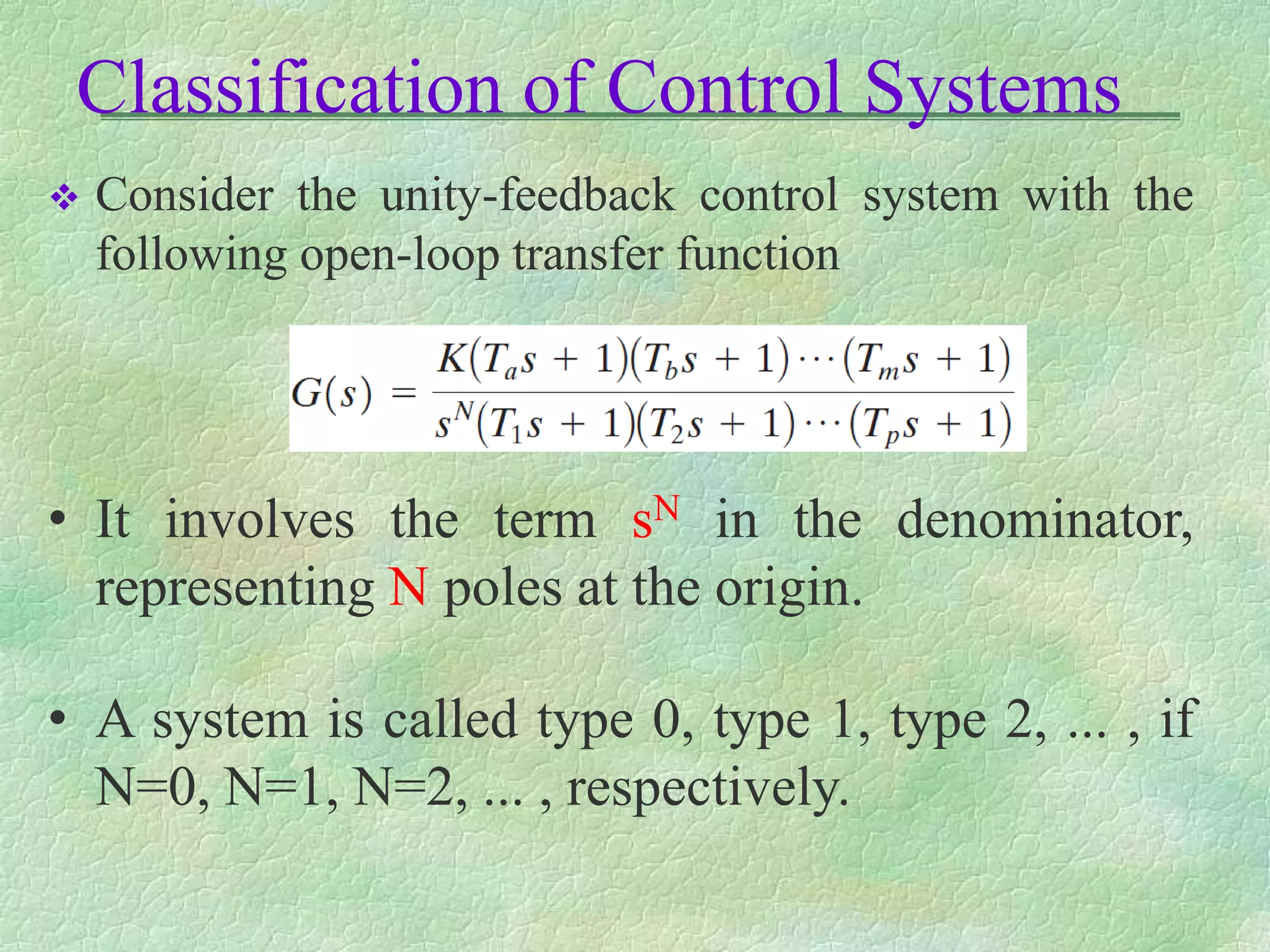
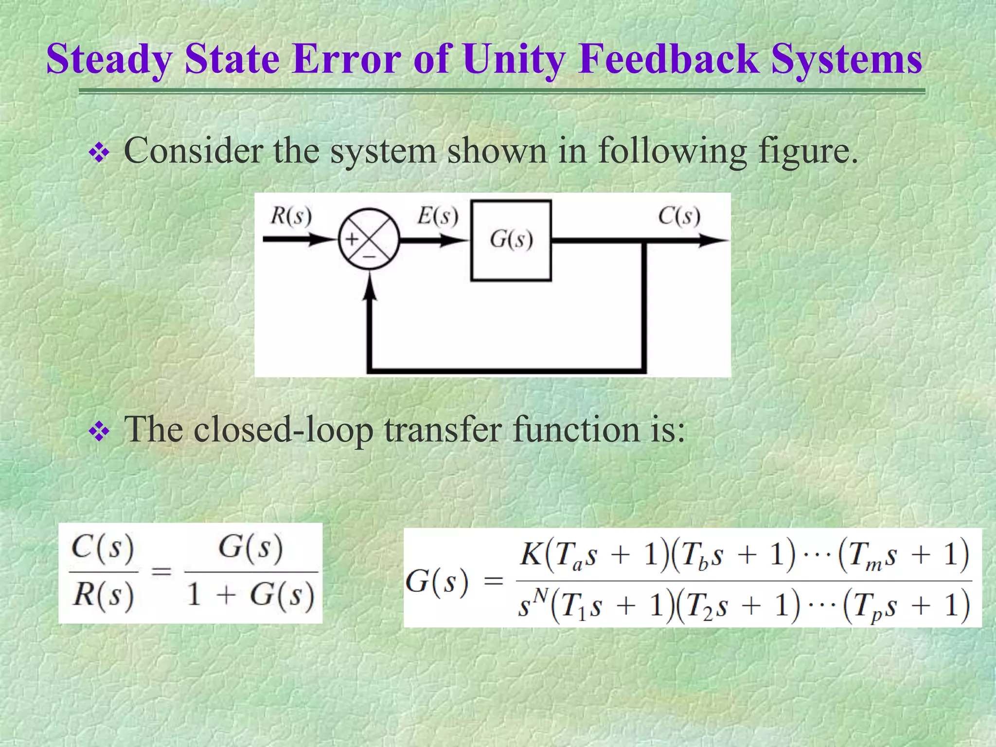
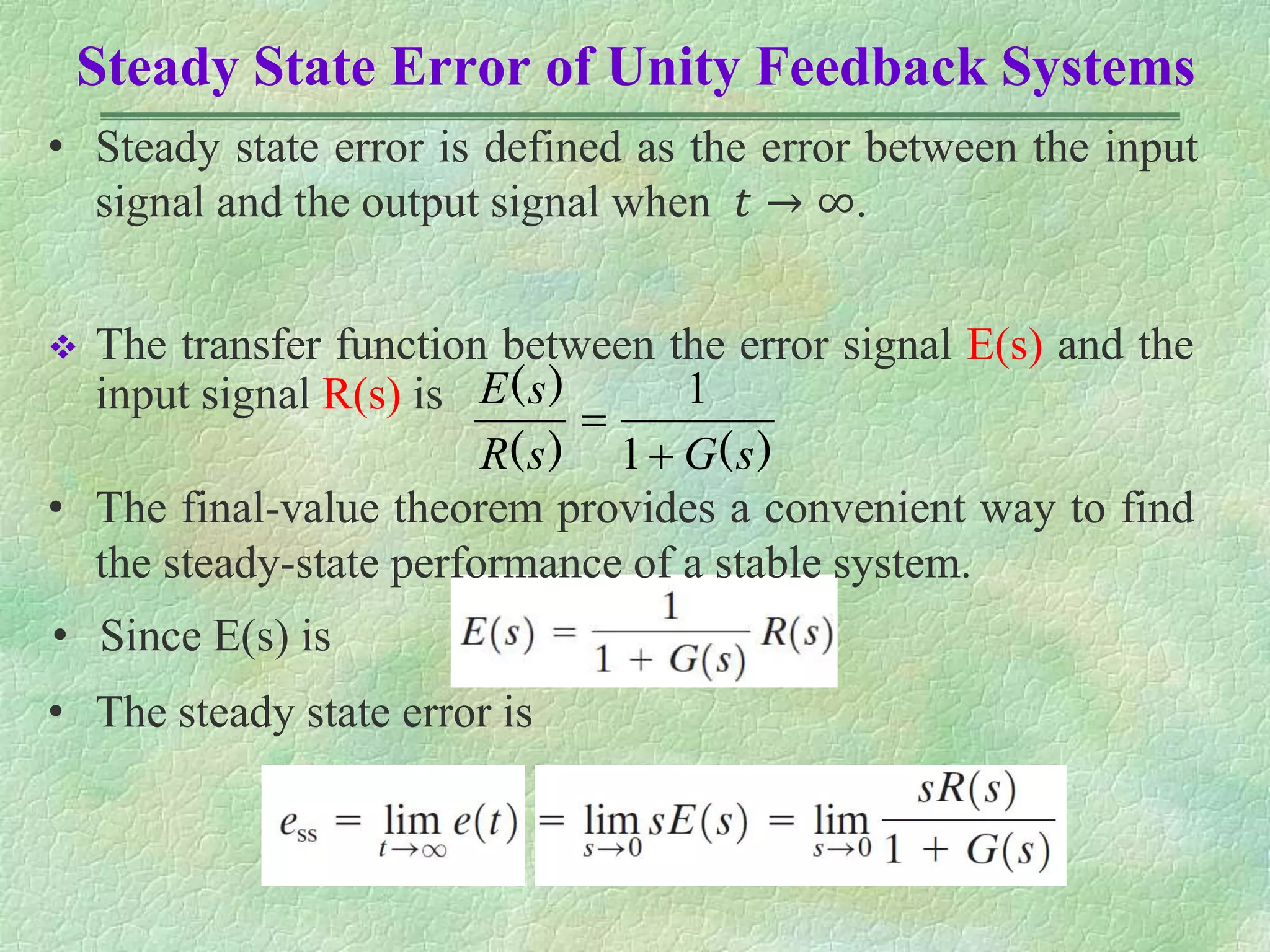
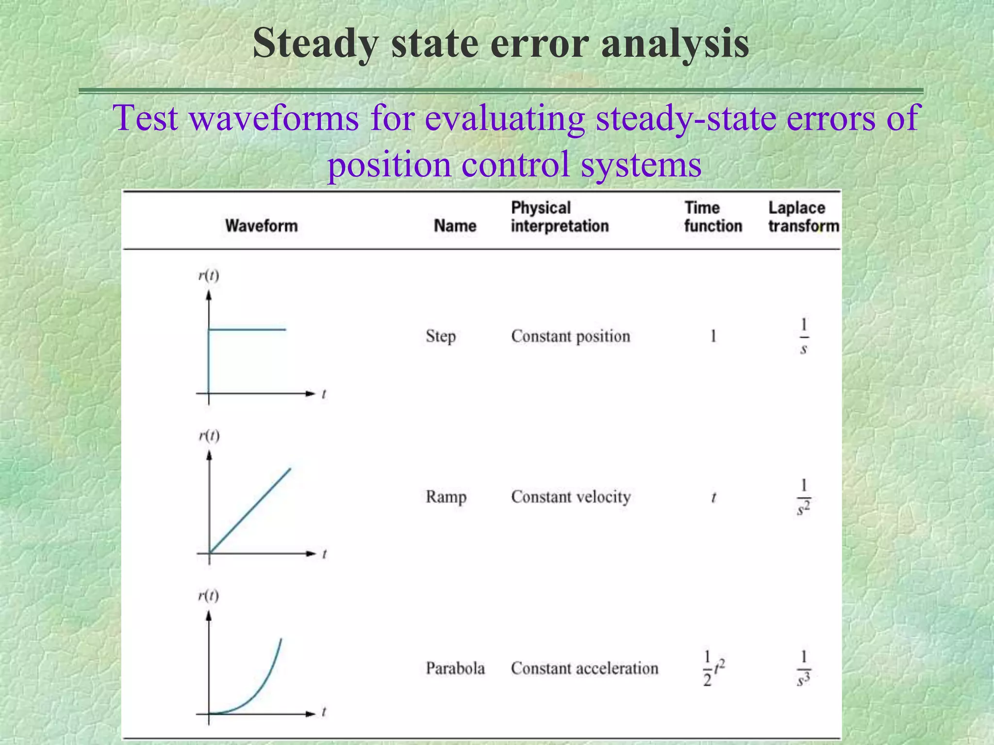
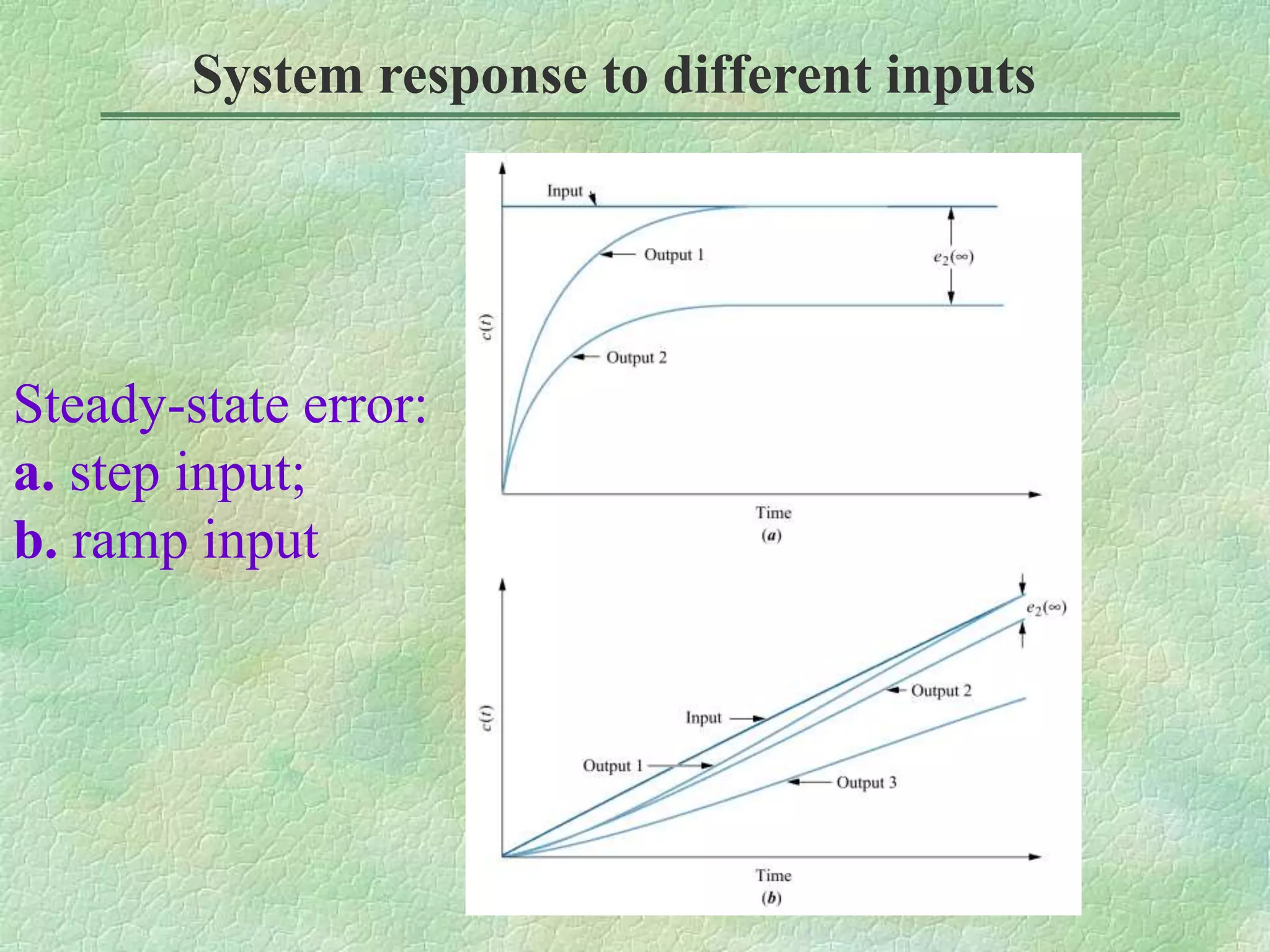
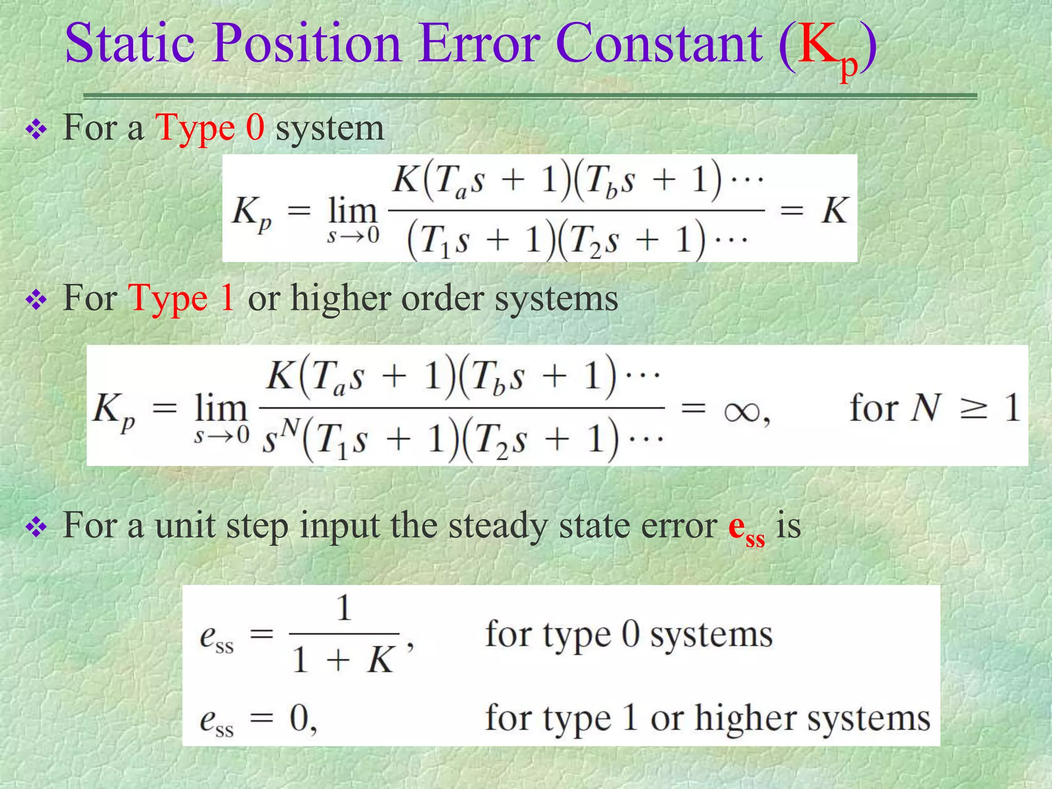
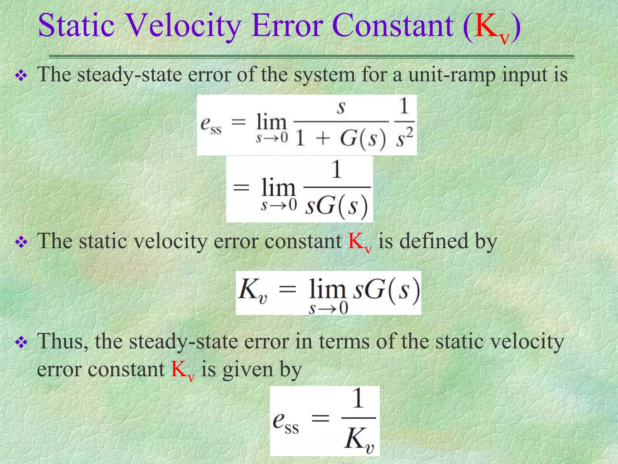
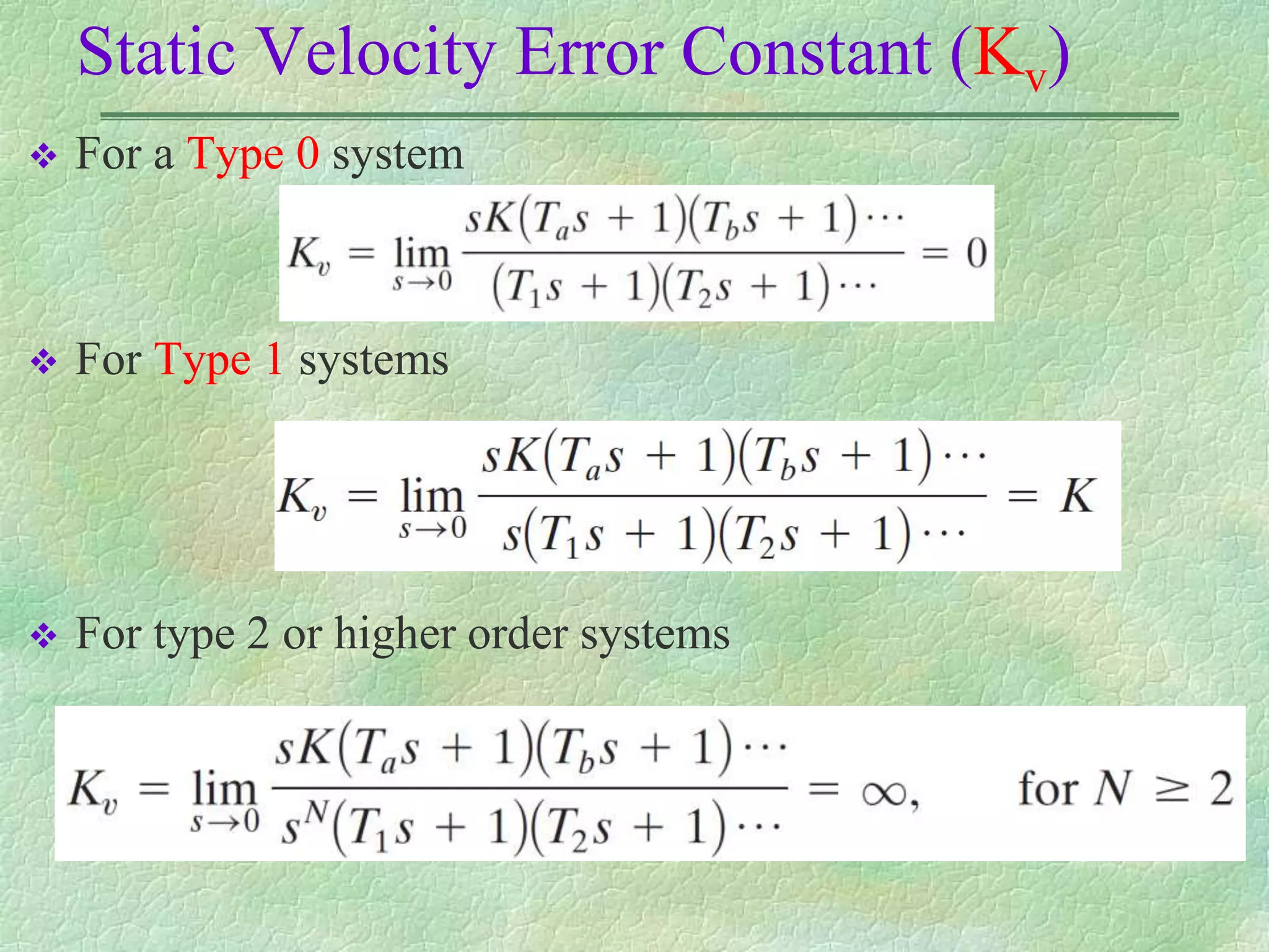
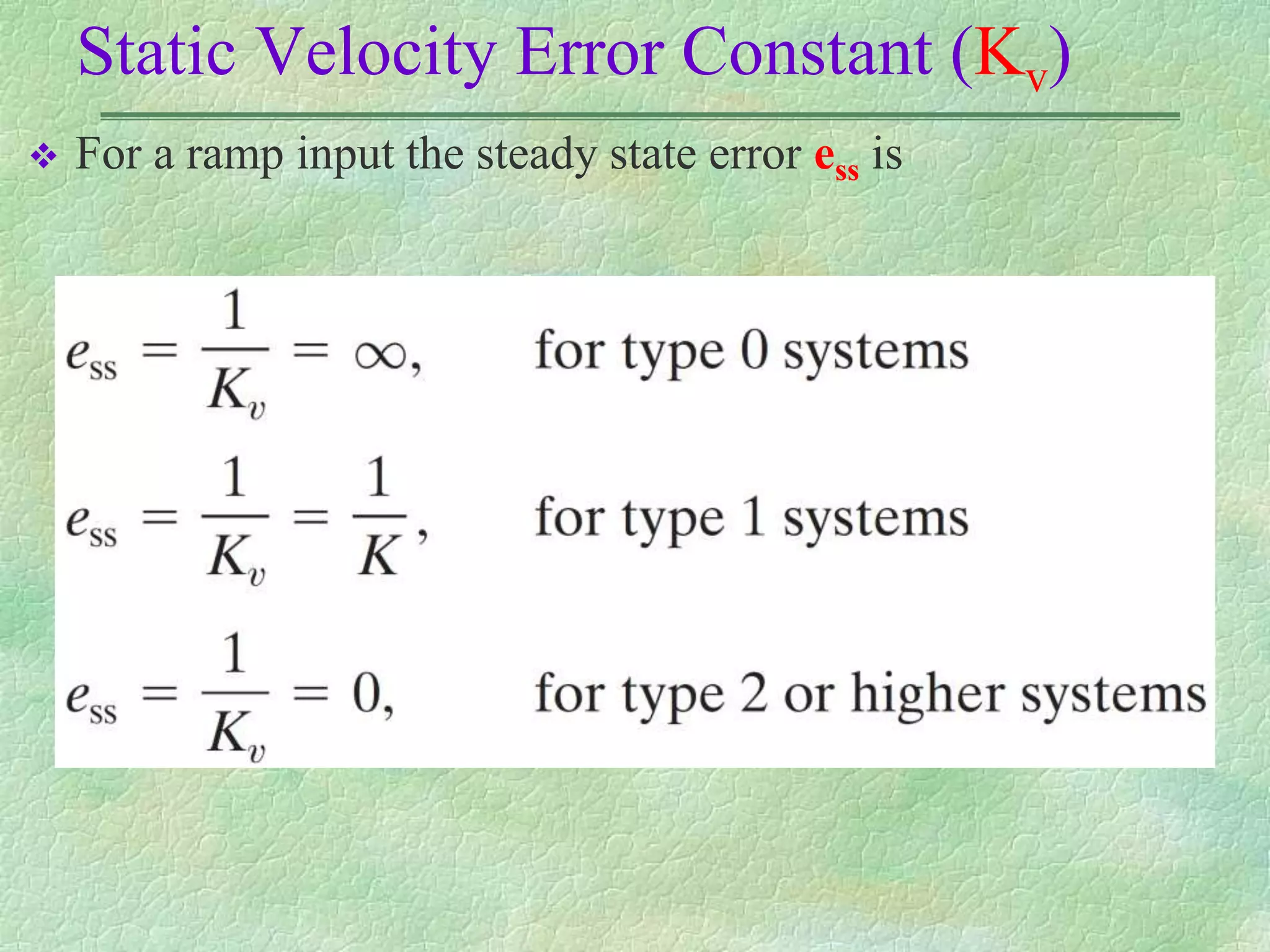
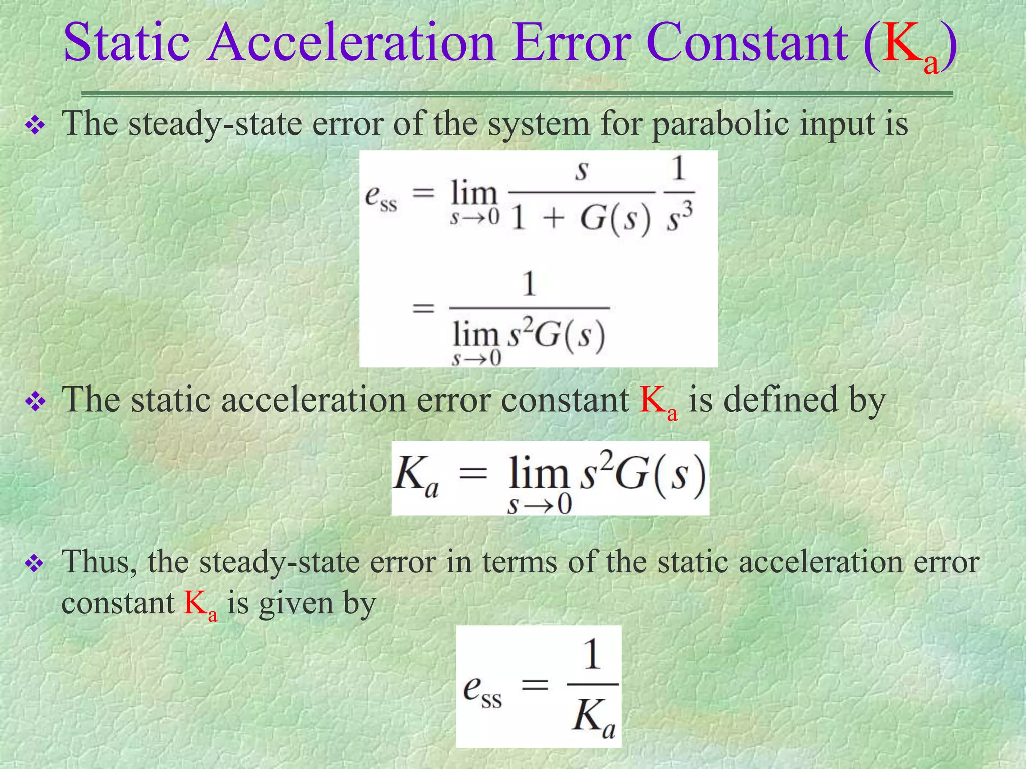
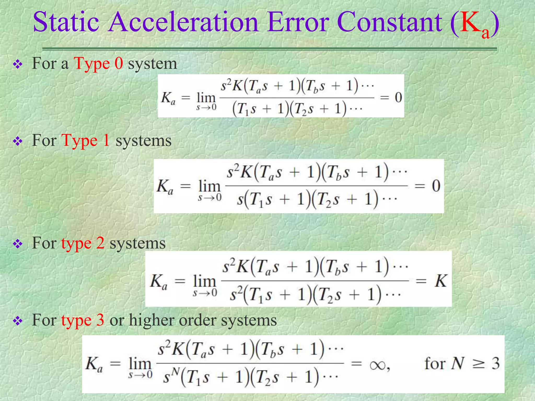
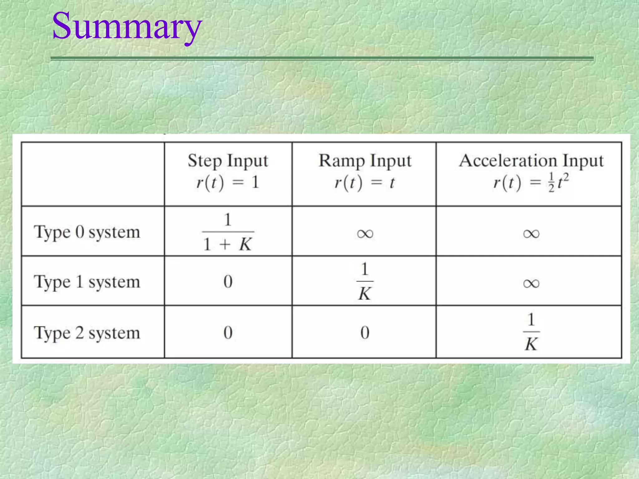
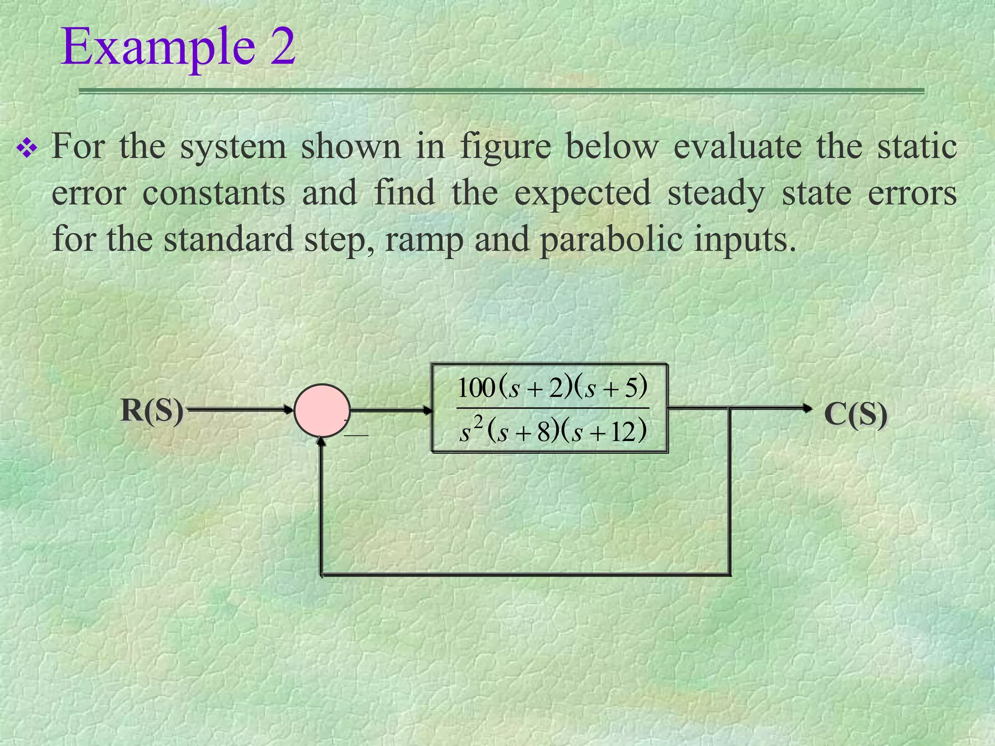
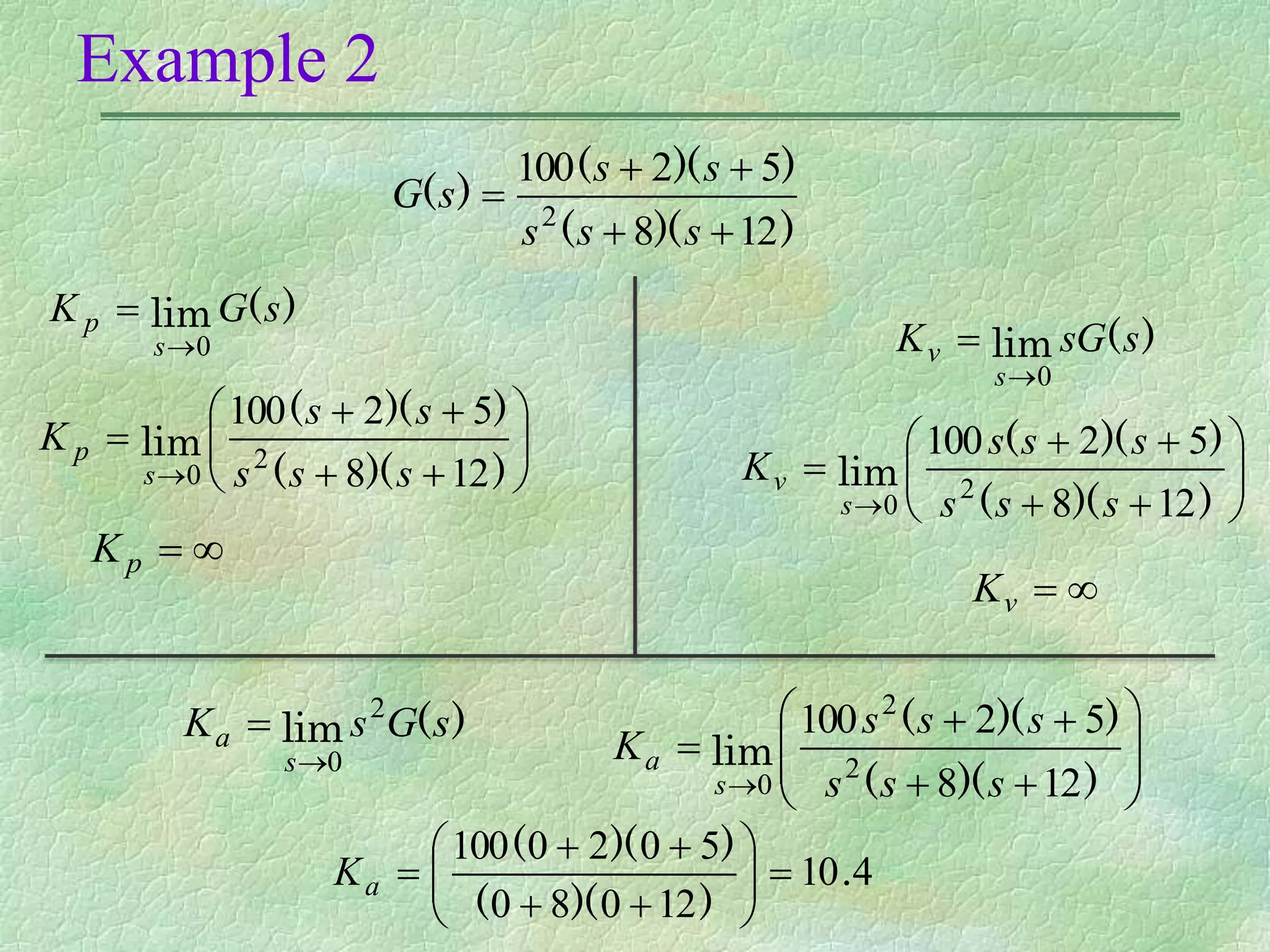
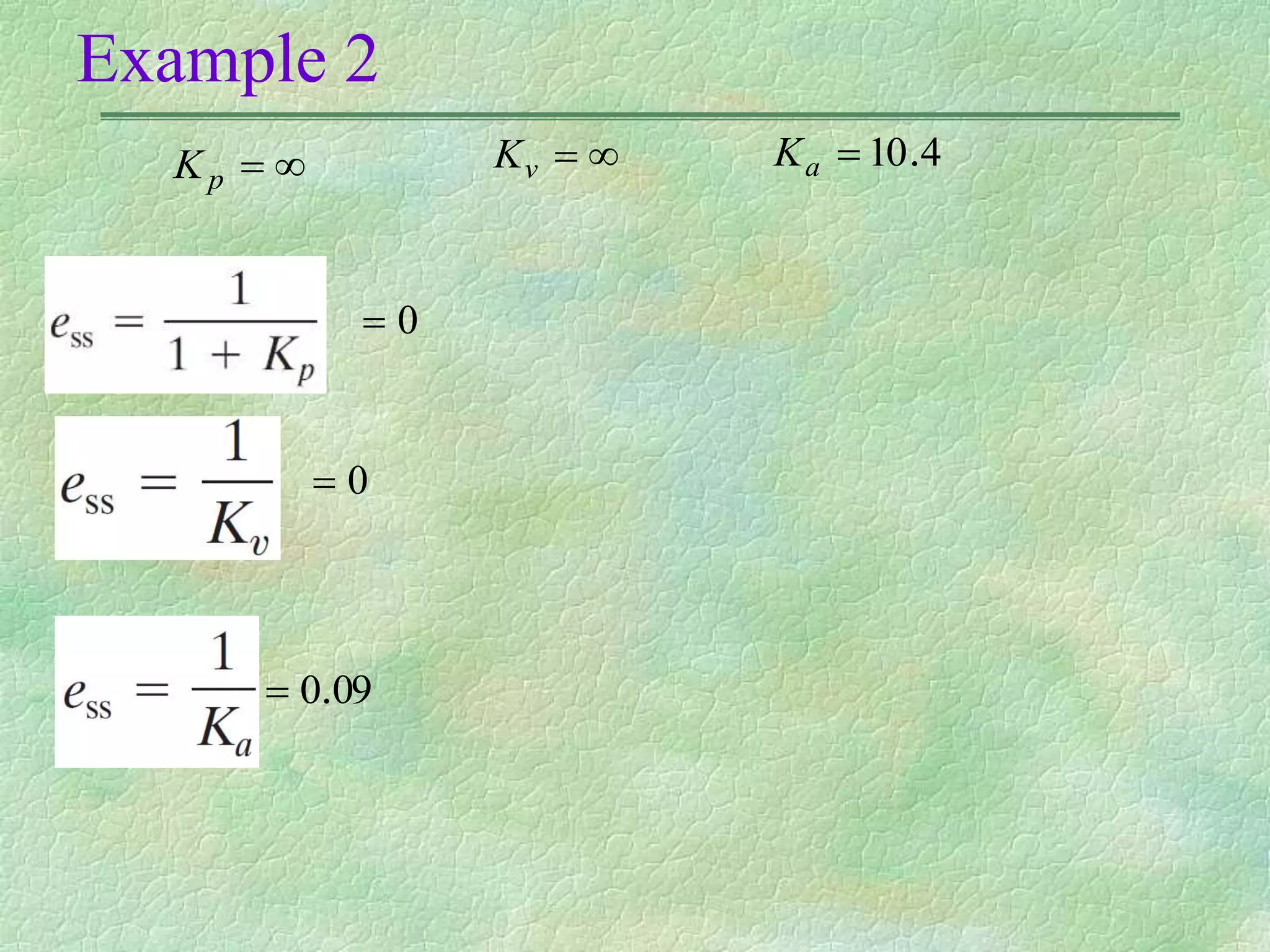
1. CONTROL SYSTEM
PRRFORMANCE
Dr.Ziad Saeed Alsaleem
2019-2020

2. Classification of Control Systems
 Consider the unity-feedback control system with the
following open-loop transfer function
• It involves the term sN in the denominator,
representing N poles at the origin.
• A system is called type 0, type 1, type 2, ... , if
N=0, N=1, N=2, ... , respectively.

3. Classification of Control Systems
 As the type number is increased, accuracy is improved.
 However, increasing the type number aggravates the
stability problem.
 A compromise between steady-state accuracy and
relative stability is always necessary.

4. Steady State Error of Unity Feedback Systems
 Consider the system shown in following figure.
 The closed-loop transfer function is:

5. Steady State Error of Unity Feedback Systems
 The transfer function between the error signal E(s) and the
input signal R(s) is
)
(
)
(
)
(
s
G
s
R
s
E


1
1
• The final-value theorem provides a convenient way to find
the steady-state performance of a stable system.
• Since E(s) is
• The steady state error is
• Steady state error is defined as the error between the input
signal and the output signal when 𝑡 → ∞.

6. Test waveforms for evaluating steady-state errors of
position control systems
Steady state error analysis

7. Steady-state error:
a. step input;
b. ramp input
System response to different inputs

8. Static Error Constants
 The static error constants are figures of merit of control
systems. The higher the constants, the smaller the steady-
state error.
 In a given system, the output may be the position,
velocity, pressure, temperature, or the like.
 Therefore, in what follows, we shall call the output
“position,” the rate of change of the output “velocity,”
and so on.
 This means that in a temperature control system
“position” represents the output temperature, “velocity”
represents the rate of change of the output temperature,
and so on.

9. Static Position Error Constant (Kp)
 For a Type 0 system
 For Type 1 or higher order systems
 For a unit step input the steady state error ess is

10.  The steady-state error of the system for a unit-ramp input is
 The static velocity error constant Kv is defined by
 Thus, the steady-state error in terms of the static velocity
error constant Kv is given by
Static Velocity Error Constant (Kv)

11. Static Velocity Error Constant (Kv)
 For a Type 0 system
 For Type 1 systems
 For type 2 or higher order systems

12. Static Velocity Error Constant (Kv)
 For a ramp input the steady state error ess is

13.  The steady-state error of the system for parabolic input is
 The static acceleration error constant Ka is defined by
 Thus, the steady-state error in terms of the static acceleration error
constant Ka is given by
Static Acceleration Error Constant (Ka)

14. Static Acceleration Error Constant (Ka)
 For a Type 0 system
 For Type 1 systems
 For type 2 systems
 For type 3 or higher order systems

15. Static Acceleration Error Constant (Ka)
 For a parabolic input the steady state error ess is

16. Summary

17. Example 2
 For the system shown in figure below evaluate the static
error constants and find the expected steady state errors
for the standard step, ramp and parabolic inputs.
C(S)
R(S) -
)
)(
(
)
)(
(
12
8
5
2
100
2




s
s
s
s
s

18. Example 2
)
)(
(
)
)(
(
)
(
12
8
5
2
100
2





s
s
s
s
s
s
G
)
(
lim s
G
K
s
p
0















 )
)(
(
)
)(
(
lim
12
8
5
2
100
2
0 s
s
s
s
s
K
s
p


p
K
)
(
lim s
sG
K
s
v
0















 )
)(
(
)
)(
(
lim
12
8
5
2
100
2
0 s
s
s
s
s
s
K
s
v


v
K
)
(
lim s
G
s
K
s
a
2
0















 )
)(
(
)
)(
(
lim
12
8
5
2
100
2
2
0 s
s
s
s
s
s
K
s
a
4
10
12
0
8
0
5
0
2
0
100
.
)
)(
(
)
)(
(














a
K

19. Example 2


p
K 

v
K 4
10.

a
K
0

0

09
0.
