This document provides a summary of a book on statistical signal processing and estimation theory. It discusses key topics covered in the book including minimum variance unbiased estimation, the Cramer-Rao lower bound, linear models, general minimum variance unbiased estimation, best linear unbiased estimation, maximum likelihood estimation, least squares estimation, the method of moments, Bayesian estimation approaches, linear Bayesian estimators such as Wiener filtering, Kalman filtering, and extensions for complex data and parameters. The book is intended as a textbook for graduate students in signal processing and provides both theoretical background and practical examples of parameter estimation techniques.
![xii PREFACE
and matrix algebra. This book can also be used for self-study and so should be useful
to the practicing engin.eer as well as the student.
The author would like to acknowledge the contributions of the many people who
over the years have provided stimulating discussions of research problems, opportuni-
ties to apply the results of that research, and support for conducting research. Thanks
are due to my colleagues L. Jackson, R. Kumaresan, L. Pakula, and D. Tufts of the
University of Rhode Island, and 1. Scharf of the University of Colorado. Exposure to
practical problems, leading to new research directions, has been provided by H. Wood-
sum of Sonetech, Bedford, New Hampshire, and by D. Mook, S. Lang, C. Myers, and
D. Morgan of Lockheed-Sanders, Nashua, New Hampshire. The opportunity to apply
estimation theory to sonar and the research support of J. Kelly of the Naval Under-
sea Warfare Center, Newport, Rhode Island, J. Salisbury of Analysis and Technology,
Middletown, Rhode Island (formerly of the Naval Undersea Warfare Center), and D.
Sheldon of th.e Naval Undersea Warfare Center, New London, Connecticut, are also
greatly appreciated. Thanks are due to J. Sjogren of the Air Force Office of Scientific
Research, whose continued support has allowed the author to investigate the field of
statistical estimation. A debt of gratitude is owed to all my current and former grad-
uate students. They have contributed to the final manuscript through many hours of
pedagogical and research discussions as well as by their specific comments and ques-
tions. In particular, P. Djuric of the State University of New York proofread much
of the manuscript, and V. Nagesha of the University of Rhode Island proofread the
manuscript and helped with the problem solutions.
Steven M. Kay
University of Rhode Island
Kingston, RI 02881
r
t
Chapter 1
Introduction
1.1 Estimation in Signal Processing
Modern estimation theory can be found at the heart of many electronic signal processing
systems designed to extract information. These systems include
1. Radar
2. Sonar
3. Speech
4. Image analysis
5. Biomedicine
6. Communications
7. Control
8. Seismology,
and all share the common problem of needing to estimate the values of a group of pa-
rameters. We briefly describe the first three of these systems. In radar we are mterested
in determining the position of an aircraft, as for example, in airport surveillance radar
[Skolnik 1980]. To determine the range R we transmit an electromagnetic pulse that is
reflected by the aircraft, causin an echo to be received b the antenna To seconds later~
as shown in igure 1.1a. The range is determined by the equation TO = 2R/c, where
c is the speed of electromagnetic propagation. Clearly, if the round trip delay To can
be measured, then so can the range. A typical transmit pulse and received waveform
a:e shown in Figure 1.1b. The received echo is decreased in amplitude due to propaga-
tIon losses and hence may be obscured by environmental nois~. Its onset may also be
perturbed by time delays introduced by the electronics of the receiver. Determination
of the round trip delay can therefore require more than just a means of detecting a
jump in the power level at the receiver. It is important to note that a typical modern
l](https://image.slidesharecdn.com/fundamentalsofstatisticalsignalprocessing-estimationtheory-kay-230513154707-1f7652e0/75/Fundamentals-Of-Statistical-Signal-Processing-Estimation-Theory-Kay-pdf-5-2048.jpg)
![2
Transmit/
receive
antenna
Transmit pulse
'-----+01 Radar processing
system
(a) Radar
....................... - - .................... -- ... -1
Received waveform
:---------_ ... -_... _-------,
TO ~--------- ... ------ .. -- __ ..!
CHAPTER 1. INTRODUCTION
Time
Time
(b) Transmit and received waveforms
Figure 1.1 Radar system
radar s!,stem will input the received continuous-time waveform into a digital computer
by takmg samples via an analog-to-digital convertor. Once the waveform has been
sampled, the data compose a time series. (See also Examples 3.13 and 7.15 for a more
detailed description of this problem and optimal estimation procedures.)
Another common application is in sonar, in which we are also interested in the
posi~ion of a target, such as a submarine [Knight et al. 1981, Burdic 1984] . A typical
passive sonar is shown in Figure 1.2a. The target radiates noise due to machiner:y
on board, propellor action, etc. This noise, which is actually the signal of interest,
propagates through the water and is received by an array of sensors. The sensor outputs
1.1. ESTIMATION IN SIGNAL PROCESSING 3
Sea surface
Towed array
Sea bottom
---------------~~---------------------------~
(a) Passive sonar
Sensor 1 output
~ Time
~'C7~ Time
Sensor 3 output
f ~ ~ / Time
(b) Received signals at array sensors
Figure 1.2 Passive sonar system
are then transmitted to a tow ship for input to a digital computer. Because of the
positions of the sensors relative to the arrival angle of the target signal, we receive
the signals shown in Figure 1.2b. By measuring TO, the delay between sensors, we can
determine the bearing f3 Z<!T t~e ~~ress.!.o~
(
eTO)
f3 = arccos d (1.1)
where c is the speed of sound in water and d is the distance between sensors (see
Examples 3.15 and 7.17 for a more detailed description). Again, however, the received](https://image.slidesharecdn.com/fundamentalsofstatisticalsignalprocessing-estimationtheory-kay-230513154707-1f7652e0/75/Fundamentals-Of-Statistical-Signal-Processing-Estimation-Theory-Kay-pdf-6-2048.jpg)
![4 CHAPTER 1. INTRODUCTION
-..... :~
<0
-.....
"&
0
.;, -1
-2
-3
0 2 4 6 8 10 12 14 16 18 20
Time (ms)
o 8 10 14
Time (ms)
Figure 1.3 Examples of speech sounds
waveforms are not "clean" as shown in Figure 1.2b but are embedded in noise, making,
the determination of To more difficult. The value of (3 obtained from (1.1) is then onli(
an estimate.
- Another application is in speech processing systems [Rabiner and Schafer 1978].
A particularly important problem is speech recognition, which is the recognition of
speech by a machine (digital computer). The simplest example of this is in recognizing
individual speech sounds or phonemes. Phonemes are the vowels, consonants, etc., or
the fundamental sounds of speech. As an example, the vowels /al and /e/ are shown
in Figure 1.3. Note that they are eriodic waveforms whose eriod is called the pitch.
To recognize whether a sound is an la or an lei the following simple strategy might
be employed. Have the person whose speech is to be recognized say each vowel three
times and store the waveforms. To reco nize the s oken vowel com are it to the
stored vowe s and choose the one that is closest to the spoken vowel or the one that
1.1. ESTIMATION IN SIGNAL PROCESSING
S
:s
-.....
<0
-.....
<0
....
.,
u
"
C.
"'
u.
p.. -10
...:l
"'0 -20
<=
:d
-30~
S
E !
!?!' -40-+
-0 !
c -50 I
.;::
" 0
p..
S
::=.. 30
1
-.....
'" 2°i
-.....
<0
t 10-+
u
::;
C.
0
'"
U
"- -10
...:l
"2 -20
id I
~ -30
1
i
500 1000 1500
Frequency (Hz)
2000
I
2500
~ -40-+
~ -50il--------~I--------_r1--------TI--------T-------~----
0:: 0 500 1000 1500 2000 2500
Frequency (Hz)
Figure 1.4 LPC spectral modeling
5
minimizes some distance measure. Difficulties arise if the itch of the speaker's voice
c anges from the time he or s e recor s the sounds (the training session) to the time
when the speech recognizer is used. This is a natural variability due to the nature of
human speech. In practice, attributes, other than the waveforms themselves, are used
to measure distance. Attributes are chosen that are less sllsceptible to variation. For
example, the spectral envelope will not change with pitch since the Fourier transform
of a periodic signal is a sampled version of the Fourier transform of one period of the
signal. The period affects only the spacing between frequency samples, not the values.
To extract the s ectral envelo e we em 10 a model of s eech called linear predictive
coding LPC). The parameters of the model determine the s ectral envelope. For the
speec soun SIll 19ure 1.3 the power spectrum (magnitude-squared Fourier transform
divided by the number of time samples) or periodogram and the estimated LPC spectral
envelope are shown in Figure 1.4. (See Examples 3.16 and 7.18 for a description of how](https://image.slidesharecdn.com/fundamentalsofstatisticalsignalprocessing-estimationtheory-kay-230513154707-1f7652e0/75/Fundamentals-Of-Statistical-Signal-Processing-Estimation-Theory-Kay-pdf-7-2048.jpg)
![6 CHAPTER 1. INTRODUCTION
the parameters of the model are estimated and used to find the spectral envelope.) It
is interesting that in this example a human interpreter can easily discern the spoken
vowel. The real problem then is to design a machine that is able to do the same. In
the radar/sonar problem a human interpreter would be unable to determine the target
position from the received waveforms, so that the machine acts as an indispensable
tool.
In all these systems we are faced with the problem of extracting values of parameters
bas~ on continuous-time waveforms. Due to the use of di ital com uters to sample
and store e contmuous-time wave orm, we have the equivalent problem of extractin
parameter values from a discrete-time waveform or a data set. at ematically, we have
the N-point data set {x[O], x[I], ... ,x[N -In which depends on an unknown parameter
(). We wish to determine () based on the data or to define an estimator
{J = g(x[O],x[I], ... ,x[N - 1]) (1.2)
where 9 is some function. This is the problem of pammeter estimation, which is the
subject of this book. Although electrical engineers at one time designed systems based
on analog signals and analog circuits, the current and future trend is based on discrete-
time signals or sequences and digital circuitry. With this transition the estimation
problem has evolved into one of estimating a parameter based on a time series, which
is just a discrete-time process. Furthermore, because the amount of data is necessarily
finite, we are faced with the determination of 9 as in (1.2). Therefore, our problem has
now evolved into one which has a long and glorious history, dating back to Gauss who
in 1795 used least squares data analysis to predict planetary m(Wements [Gauss 1963
(English translation)]. All the theory and techniques of statisti~al estimation are at
our disposal [Cox and Hinkley 1974, Kendall and Stuart 1976-1979, Rao 1973, Zacks
1981].
Before concluding our discussion of application areas we complete the previous list.
4. Image analysis - Elstimate the position and orientation of an object from a camera
image, necessary when using a robot to pick up an object [Jain 1989]
5. Biomedicine - estimate the heart rate of a fetu~ [Widrow and Stearns 1985]
6. Communications - estimate the carrier frequency of a signal so that the signal can
be demodulated to baseband [Proakis 1983]
1. Control - estimate the position of a powerboat so that corrective navigational
action can be taken, as in a LORAN system [Dabbous 1988]
8. Seismology - estimate the underground distance of an oil deposit based on SOUD&
reflections dueto the different densities of oil and rock layers [Justice 1985].
Finally, the multitude of applications stemming from analysis of data from physical
experiments, economics, etc., should also be mentioned [Box and Jenkins 1970, Holm
and Hovem 1979, Schuster 1898, Taylor 1986].
1.2. THE MATHEMATICAL ESTIMATION PROBLEM 7
x[O]
Figure 1.5 Dependence of PDF on unknown parameter
1.2 The Mathematical Estimation Problem
In determining good .estimators the first step is to mathematically model the data.
~ecause the data are mherently random, we describe it by it§, probability density func-
tion (PDF) 01:" p(x[O], x[I], ... ,x[N - 1]; ()). The PDF is parameterized by the unknown
l2arameter ()J I.e., we have a class of PDFs where each one is different due to a different
value of (). We will use a semicolon to denote this dependence. As an example, if N = 1
and () denotes the mean, then the PDF of the data might be
p(x[O]; ()) = .:-." exp [__I_(x[O] _ ())2]
v 27rO'2 20'2
which is shown in Figure 1.5 for various values of (). It should be intuitively clear that
because the value of () affects the probability of xiO], we should be able to infer the value
of () from the observed value of x[OL For example, if the value of x[O] is negative, it is
doubtful tha~ () =:'.()2' :rhe value. (). = ()l might be more reasonable, This specification
of th~ PDF IS cntlcal m determmmg a good estima~. In an actual problem we are
not glv~n a PDF but .must choose one that is not only consistent with the problem
~onstramts and any pnor knowledge, but one that is also mathematically tractable. To
~llus~rate the appr~ach consider the hypothetical Dow-Jones industrial average shown
IP. FIgure 1.6. It. mIght be conjectured that this data, although appearing to fluctuate
WIldly, actually IS "on the average" increasing. To determine if this is true we could
assume that the data actually consist of a straight line embedded in random noise or
x[n] =A+Bn+w[n] n = 0, 1, ... ,N - 1.
~ reasonable model for the noise is that win] is white Gaussian noise (WGN) or each
sample of win] has the PDF N(0,O'2
) (denotes a Gaussian distribution with a mean
of 0 and a variance of 0'2) and is uncorrelated with all the other samples. Then, the
unknown parameters are A and B, which arranged as a vector become the vector
parameter 9 = [A Bf. Letting x = [x[O] x[I] ... x[N - lW, the PDF is
1 [1 N-l ]
p(x; 9) = (27rO'2)~ exp - 20'2 ~ (x[n]- A - Bn)2 . (1.3)
The choice of a straight line for the signal component is consistent with the knowledge
that the Dow-Jones average is hovering around 3000 (A models this) and the conjecture](https://image.slidesharecdn.com/fundamentalsofstatisticalsignalprocessing-estimationtheory-kay-230513154707-1f7652e0/75/Fundamentals-Of-Statistical-Signal-Processing-Estimation-Theory-Kay-pdf-8-2048.jpg)
![8 CHAPTER 1. INTRODUCTION
3200
3150
~
<'$
3100
...
" 3050
~
'Il
3000
"
~
0
.-, 2950
~
0
2900
0
2850
2800
0 10 20 30 40 50 60 70 80 90 100
Day number
Figure 1.6 Hypothetical Dow-Jones average
that it is increasing (B > 0 models this). The assumption of WGN is justified by the
need to formulate a mathematically tractable model so that closed form estimators can
be found. Also, it is reasonable unless there is strong evidence to the contrary, such as
highly correlated noise. Of course, the performance of any estimator obtained will be
critically dependent on the PDF assum tions. We can onl hope the estimator obtained
is robust, in that slight changes in the PDF do not severely affect t per ormance of the
estimator. More conservative approaches utilize robust statistical procedures [Huber
1981J.
Estimation based on PDFs such as (1.3) is termed classical estimation in that the
parameters of interest are assumed to be deterministic but unknown. In the Dow-Jo~
average example we know a priori that the mean is somewhere around 3000. It seems
inconsistent with reality, then, to choose an estimator of A that can result in values as
low as 2000 or as high as 4000. We might be more willing to constrain the estimator
to produce values of A in the range [2800, 3200J. To incorporate this prior knowledge
we can assume that A is no Ion er deterministic but a random variable and assign it a
DF, possibly uni orm over the [2800, 3200J interval. Then, any subsequent estImator
will yield values in this range. Such an approach is termed Bayesian estimation. The
parameter we are attem tin to estimate is then viewed as a realization of the randQ;
, the data are described by the joint PDF
p(x,9) =p(xI9)p(9)
1.3. ASSESSING ESTIMATOR PERFORMANCE
3.0
i
2.5-+
1.0
"F.
fl 0.5
0.0
-1.0
-1.5
-{)'5~
-2.0-r--'I--il--il--il--il--II--II__"1'I__-+1----<1
o ill W ~ ~ M W m W 00 ~
n
Figure 1.7 Realization of DC level in noise
Once the PDF has been specified the problem becomes one f d t ..
" . ' 0 e ermmmg an
optImal estImator or functlOn of the data as in (1 2) Note that t' t
' . . an es Ima or may
depend on other par~meters, but only if they are known. An estimator may be thought
of as a rule that ~Sl ns a value to 9 for each realization of x. The estimate of 9 is
the va ue o. 9 obtal~ed .for a given realization of x. This distinction is analogous to a
random vanable (whIch IS a f~nction defined on the sample space) and the value it takes
on. Althoug~ some authors dIstinguish between the two by using capital and lowercase
letters, we WIll not do so. The meaning will, hopefully, be clear from the context.
1.3 Assessing Estimator Performance
Consider.the data set shown in Figure 1.7. From a cursory inspection it appears that
x[n] conslst~ of.a DC.level A in noise. (The use of the term DC is in reference to direct
current, whIch IS eqUlvalent to the constant function.) We could model the data as
x[nJ =A +wIn]
;~re w n denotes so~e zero ~ean noise ro~~ss. B~ed on the data set {x[O], x[1], .. .,
(
[[ .l]), we would .hke to estImate A. IntUltlvely, smce A is the average level of x[nJ
w nJ IS zero mean), It would be reasonable to estimate A as
I N-l
.4= N Lx[nJ
n=O
or by the sample mean of the data. Several questions come to mind:
I 1. How close will .4 be to A?
' 2. Are there better estimators than the sample mean?
9](https://image.slidesharecdn.com/fundamentalsofstatisticalsignalprocessing-estimationtheory-kay-230513154707-1f7652e0/75/Fundamentals-Of-Statistical-Signal-Processing-Estimation-Theory-Kay-pdf-9-2048.jpg)
![10 CHAPTER 1. INTRODUCTION
For the data set in Figure 1.7 it turns out that .1= 0.9, which is close to the true value
of A = 1. Another estimator might be
A=x[o].
Intuitively, we would not expect this estimator to perform as well since it does not
make use of all the data. There is no averaging to reduce the noise effects. However,
for the data set in Figure 1.7, A = 0.95, which is closer to the true value of A than
the sample mean estimate. Can we conclude that A is a better estimator than A?
The answer is of course no. Because an estimator is a function of the data, which
are random variables, it too is a random variable, subject to many possible outcomes.
The fact that A is closer to the true value only means that for the given realization of
data, as shown in Figure 1.7, the estimate A = 0.95 (or realization of A) is closer to
the true value than the estimate .1= 0.9 (or realization of A). To assess performance
we must do so statistically. One possibility would be to repeat the experiment that
generated the data and apply each estimator to every data set. Then, we could ask
which estimator produces a better estimate in the majority of the cases. Suppose we
repeat the experiment by fixing A =1 and adding different noise realizations of win] to
generate an ensemble of realizations of x[n]. Then, we determine the values of the two
estimators for each data set and finally plot the histograms. (A histogram describes the
number of times the estimator produces a given range of values and is an approximation
to the PDF.) For 100 realizations the histograms are shown in Figure 1.8. It should
now be evident that A is a better estimator than A because the values obtained are
more concentrated about the true value of A =1. Hence, Awill uliWl-lly produce a value
closer to the true one than A. The skeptic, however, might argue-that if we repeat the
experiment 1000 times instead, then the histogram of A will be more concentrated. To
dispel this notion, we cannot repeat the experiment 1000 times, for surely the skeptic
would then reassert his or her conjecture for 10,000 experiments. To prove that A is
better we could establish that the variance is less. The modeling assumptions that we
must employ are that the w[n]'s, in addition to being zero mean, are uncorrelated and
have equal variance u 2
. Then, we first show that the mean of each estimator is the true
value or
(
1 N-l )
E(A) E N ~ x[nJ
1 N-l
= N L E(x[n])
n=O
A
E(A) E(x[O])
A
so that on the average the estimators produce the true value. Second, the variances are
(
1 N-l )
var(A) = var N ~ x[nJ
1.3. ASSESSING ESTIMATOR PERFORMANCE
30
r
'" 25j
'0 15
lil
1
20
j
r:~i------rl- r - I------;--------1~JI~m---r---I_
-3 -2 -1 0 2 ~
-1
Sample mean value, A
o
'I
1
i
I
First sample value, A
2 3
Figure 1.8 Histograms for sample mean and first sample estimator
1 N-l
N2 L var(x[nJ)
n=O
1 2
N2
Nu
u2
N
since the w[nJ's are uncorrelated and thus
var(A) var(x[OJ)
u2
> var(A).
11](https://image.slidesharecdn.com/fundamentalsofstatisticalsignalprocessing-estimationtheory-kay-230513154707-1f7652e0/75/Fundamentals-Of-Statistical-Signal-Processing-Estimation-Theory-Kay-pdf-10-2048.jpg)
![12 CHAPTER 1. INTRODUCTION
Furthermore, if we could assume that w[n] is Gaussian, we could also conclude that the
probability of a given magnitude error is less for A. than for A (see Problem 2.7).
ISeveral important points are illustrated by the previous example, which should
always be ept in mind.
1. An estimator is a random variable. As such, its erformance can onl be com-
pletely descri e statistical y or by its PDF.
2. The use of computer simulations for assessing estimation performance, although
quite valuable for gaiiiing insight and motivating conjectures, is never conclusive.
At best, the true performance may be obtained to the desired degree of accuracy.
At worst, for an insufficient number of experiments and/or errors in the simulation
techniques employed, erroneous results may be obtained (see Appendix 7A for a
further discussion of Monte Carlo computer techniques).
Another theme that we will repeatedly encounter is the tradeoff between perfor:
mance and computational complexity. As in the previous example, even though A
has better performance, it also requires more computation. We will see that QPtimal
estimators can sometimes be difficult to implement, requiring a multidimensional opti-
mization or inte ration. In these situations, alternative estimators that are suboptimal,
but which can be implemented on a igita computer, may be preferred. For any par-
ticular application, the user must determine whether the loss in performance is offset
by the reduced computational complexity of a suboptimal estimator.
1.4 Some Notes to the Reader
Our philosophy in presenting a theory of estimation is to provide the user with the
main ideas necessary for determining optimal estimator.§. We have included results
that we deem to be most useful in practice, omitting some important theoretical issues.
The latter can be found in many books on statistical estimation theory which have
been written from a more theoretical viewpoint [Cox and Hinkley 1974, Kendall and
Stuart 1976--1979, Rao 1973, Zacks 1981]. As mentioned previously, our goal is t<;)
obtain an 0 timal estimator, and we resort to a subo timal one if the former cannot
be found or is not implementa ~. The sequence of chapters in this book follows this
approach, so that optimal estimators are discussed first, followed by approximately
optimal estimators, and finally suboptimal estimators. In Chapter 14 a "road map" for
finding a good estimator is presented along with a summary of the various estimators
and their properties. The reader may wish to read this chapter first to obtain an
overview.
We have tried to maximize insight by including many examples and minimizing
long mathematical expositions, although much of the tedious algebra and proofs have
been included as appendices. The DC level in noise described earlier will serve as a
standard example in introducing almost all the estimation approaches. It is hoped
that in doing so the reader will be able to develop his or her own intuition by building
upon previously assimilated concepts. Also, where possible, the scalar estimator is
REFERENCES 13
presented first followed by the vector estimator. This approach reduces the tendency
of vector/matrix algebra to obscure the main ideas. Finally, classical estimation is
described first, followed by Bayesian estimation, again in the interest of not obscuring
the main issues. The estimators obtained using the two approaches, although similar
in appearance, are fundamentally different.
The mathematical notation for all common symbols is summarized in Appendix 2.
The distinction between a continuous-time waveform and a discrete-time waveform or
sequence is made through the symbolism x(t) for continuous-time and x[n] for discrete-
time. Plots of x[n], however, appear continuous in time, the points having been con-
nected by straight lines for easier viewing. All vectors and matrices are boldface with
all vectors being column vectors. All other symbolism is defined within the context of
the discussion.
References
Box, G.E.P., G.M. Jenkins, Time Series Analysis: Forecasting and Contro~ Holden-Day, San
Francisco, 1970.
Burdic, W.S., Underwater Acoustic System Analysis, Prentice-Hall, Englewood Cliffs, N.J., 1984.
Cox, D.R., D.V. Hinkley, Theoretical Statistics, Chapman and Hall, New York, 1974.
Dabbous, T.E., N.U. Ahmed. J.C. McMillan, D.F. Liang, "Filtering of Discontinuous Processes
Arising in Marine Integrated Navigation," IEEE Trans. Aerosp. Electron. Syst., Vol. 24,
pp. 85-100, 1988.
Gauss, K.G., Theory of Motion of Heavenly Bodies, Dover, New York, 1963.
Holm, S., J.M. Hovem, "Estimation of Scalar Ocean Wave Spectra by the Maximum Entropy
Method," IEEE J. Ocean Eng., Vol. 4, pp. 76-83, 1979.
Huber, P.J., Robust Statistics, J. Wiley, ~ew York, 1981.
Jain, A.K., Fundamentals of Digital Image ProceSSing, Prentice-Hall, Englewood Cliffs, N.J., 1989.
Justice, J.H.. "Array Processing in Exploration Seismology," in Array Signal Processing, S. Haykin,
ed., Prentice-HaU, Englewood Cliffs, N.J., 1985.
Kendall, Sir M., A. Stuart, The Advanced Theory of Statistics, Vols. 1-3, Macmillan, New York,
1976--1979.
Knight, W.S., RG. Pridham, S.M. Kay, "Digital Signal Processing for Sonar," Proc. IEEE, Vol.
69, pp. 1451-1506. Nov. 1981.
Proakis, J.G., Digital Communications, McGraw-Hill, New York, 1983.
Rabiner, L.R., RW. Schafer, Digital Processing of Speech Signals, Prentice-Hall, Englewood Cliffs,
N.J., 1978.
Rao, C.R, Linear Statistical Inference and Its Applications, J. Wiley, New York, 1973.
Schuster, !," "On the Investigation of Hidden Periodicities with Application to a Supposed 26 Day
.PerIod of Meterological Phenomena," Terrestrial Magnetism, Vol. 3, pp. 13-41, March 1898.
Skolmk, M.L, Introduction to Radar Systems, McGraw-Hill, ~ew York, 1980.
Taylor, S., Modeling Financial Time Series, J. Wiley, New York, 1986.
Widrow, B., Stearns, S.D., Adaptive Signal Processing, Prentice-Hall, Englewood Cliffs, N.J., 1985.
Zacks, S., Parametric Statistical Inference, Pergamon, New York, 1981.](https://image.slidesharecdn.com/fundamentalsofstatisticalsignalprocessing-estimationtheory-kay-230513154707-1f7652e0/75/Fundamentals-Of-Statistical-Signal-Processing-Estimation-Theory-Kay-pdf-11-2048.jpg)
![14
Problems
CHAPTER 1. INTRODUCTION
1. In a radar system an estimator of round trip delay To has the PDF To ~ N(To, (J~a)"
where 7< is the true value. If the range is to be estimated, propose an estimator R
and find its PDF. Next determine the standard deviation (J-ra so that 99% of th~
time the range estimate will be within 100 m of the true value. Use c = 3 x 10
mls for the speed of electromagnetic propagation.
2. An unknown parameter fJ influences the outcome of an experiment which is mod-
eled by the random variable x. The PDF of x is
p(x; fJ) = vkexp [-~(X -fJ?) .
A series of experiments is performed, and x is found to always be in the interval
[97, 103]. As a result, the investigator concludes that fJ must have been 100. Is
this assertion correct?
3. Let x = fJ +w, where w is a random variable with PDF Pw(w)..IfbfJ is (a dfJet)er~in~
istic parameter, find the PDF of x in terms of pw and denote It y P x; ... ex
assume that fJ is a random variable independent of wand find the condltlO?al
PDF p(xlfJ). Finally, do not assume that eand ware independent and determme
p(xlfJ). What can you say about p(x; fJ) versus p(xlfJ)?
4. It is desired to estimate the value of a DC level A in WGN or
x[n] = A +w[n] n = 0,1, ... , N - C
where w[n] is zero mean and uncorrelated, and each sample has variance (J2 = l.
Consider the two estimators
1 N-I
N 2:: x[n]
n=O
A =
A _1_ (2X[0] +~ x[n] +2x[N - 1]) .
N + 2 n=1
Which one is better? Does it depend on the value of A?
5. For the same data set as in Problem 1.4 the following estimator is proposed:
{
x [0]
A= ~'~x[n] A2 = A2 < 1000.
.,.2 -
The rationale for this estimator is that for a high enough signal-to-noise ratio
(SNR) or A2/(J2, we do not need to reduce the effect of.noise by averaging and
hence can avoid the added computation. Comment on thiS approach.
Chapter 2
Minimum Variance Unbiased
Estimation
2.1 Introduction
In this chapter we will be in our search for good estimators of unknown deterministic
parame ers. e will restrict our attention to estimators which on the average yield
the true parameter value. Then, within this class of estimators the goal will be to find
the one that exhibits the least variability. Hopefully, the estimator thus obtained will
produce values close to the true value most of the time. The notion of a minimum
variance unbiased estimator is examined within this chapter, but the means to find it
will require some more theory. Succeeding chapters will provide that theory as well as
apply it to many of the typical problems encountered in signal processing.
2.2 Summary
An unbiased estimator is defined by (2.1), with the important proviso that this holds for
all possible values of the unknown parameter. Within this class of estimators the one
with the minimum variance is sought. The unbiased constraint is shown by example
to be desirable from a practical viewpoint since the more natural error criterion, the
minimum mean square error, defined in (2.5), generally leads to unrealizable estimators.
Minimum variance unbiased estimators do not, in eneral, exist. When they do, several
methods can be used to find them. The methods reI on the Cramer-Rao ower oun
and the concept of a sufficient statistic. If a minimum variance unbiase estimator
does not exist or if both of the previous two approaches fail, a further constraint on the
estimator, to being linear in the data, leads to an easily implemented, but suboptimal,
estimato!,;
15](https://image.slidesharecdn.com/fundamentalsofstatisticalsignalprocessing-estimationtheory-kay-230513154707-1f7652e0/75/Fundamentals-Of-Statistical-Signal-Processing-Estimation-Theory-Kay-pdf-12-2048.jpg)
![16 CHAPTER 2. MINIMUM VARIANCE UNBIASED ESTIMATION
2.3 Unbiased Estimators
For an estimator to be unbiased we mean that on the average the estimator will yield
the true value of the unknown parameter. Since the parameter value may in general be
anywhere in the interval a < 8 < b, unbiasedness asserts that no matter what the true
value of 8, our estimator will yield it on the average. Mathematically, an estimator i~
~~~il •
E(iJ) = 8 (2.1)
where (a,b) denotes the range of possible values of 8.
Example 2.1 - Unbiased Estimator for DC Level in White Gaussian Noise
Consider the observatioJ!s
x[n) = A +w[n) n = 0, 1, ... ,N - 1
where A is the parameter to be estimated and w[n] is WGN. The parameter A can
take on any value in the interval -00 < A < 00. Then, a reasonable estimator for the
average value of x[n] is
or the sample mean. Due to the linearity properties of the expectation operator
[
1 N-1 ]
E(A.) = E N ~ x[n)
1 N-1
N L E(x[nJ)
n=O
N-1
~LA
n=O
= A
for all A. The sample mean estimator is therefore unbiased.
(2.2)
<>
In this example A can take on any value, although in general the values of an unknown
parameter may be restricted by physical considerations. Estimating the resistance R
of an unknown resistor, for example, would necessitate an interval 0 < R < 00.
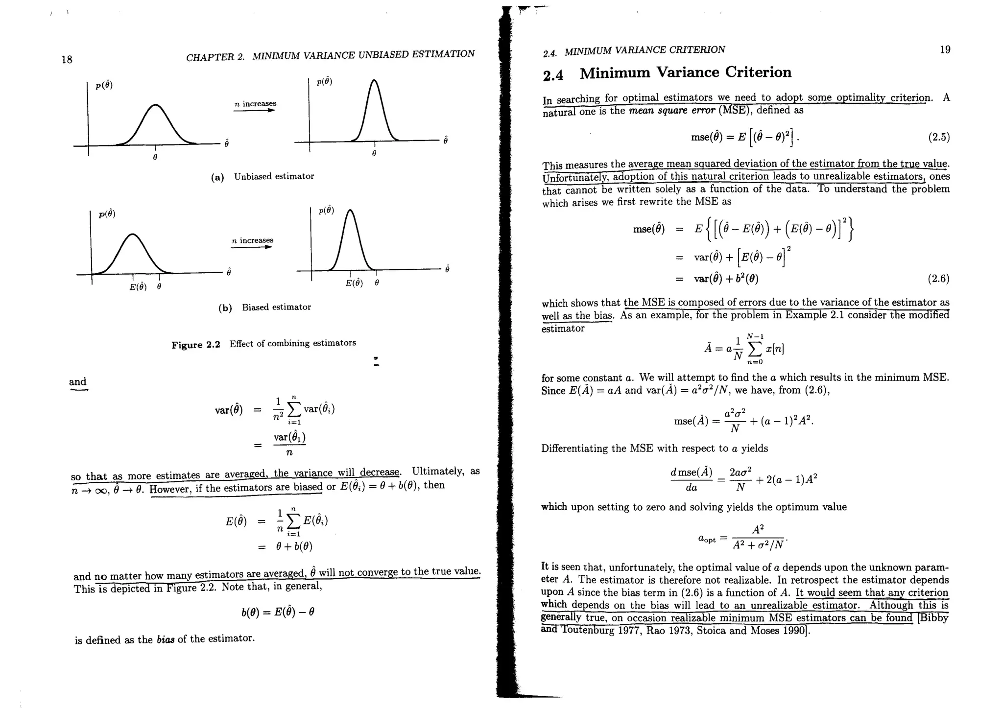
Unbiased estimators tend to have symmetric PDFs centered about the true value of
8, although this is not necessary (see Problem 2.5). For Example 2.1 the PDF is shown
in Figure 2.1 and is easily shown to be N(A, (72/N) (see Problem 2.3).
The restriction that E(iJ) =8 for all 8 is an important one. Lettin iJ =
x = [x 0 x , it asserts that
E(iJ) = Jg(x)p(x; 8) dx = 8 for all 8. (2.3)
2.3. UNBIASED ESTIMATORS 17
A
Figure 2.1 Probability density function for sample mean estimator
It is possible, however, that (2.3) may hold for some values of 8 and not others as the
next example illustrates. '
Example 2.2 - Biased Estimator for DC Level in White Noise
Consider again Example 2.1 but with the modified sample mean estimator
Then,
_ 1 N-1
A= 2N Lx[n].
E(A)
n=O
~A
2
A if A=O
# A if A # o.
It is seen that (2.3) holds for the modified estimator only for A = o. Clearly, A is a
biased estimator. <>
That an estimator is unbiased does not necessarily mean that it is a good estimator.
It only guarantees that on the average it will attain the true value. On the other hand
biased estimators are ones that are characterized by a systematic error, which presum~
ably should not be present. A persistent bias will always result in a poor estimator.
As an example, the unbiased property has an important implication when several es-
timators are combined (see Problem 2.4). ~t s?metimes occurs that multiple estimates
~th~ same paran:eter ar.e available, i.e., {81, 82 , •.. , 8n }. A reasonable procedure is to
combme these estimates mto, hopefully, a better one by averaging them to form
. 1 ~.
8=- ~8i.
n i=l
(2.4)
Assuming the estimators are unbiased, with the same variance, and uncorrelated with
each other,
E(iJ) = 8](https://image.slidesharecdn.com/fundamentalsofstatisticalsignalprocessing-estimationtheory-kay-230513154707-1f7652e0/75/Fundamentals-Of-Statistical-Signal-Processing-Estimation-Theory-Kay-pdf-13-2048.jpg)
![X[~] ~ N (f)/ 1 )
X [1] -'?- f'I C~, 1) , &;; 0 I
') N (f), 2) ) 9-.( 0 (
i1" ~ [X[,1+ x[l] )
'2
O
2 > !.. ('2. Xfr,J + X[11)
q,
ry 1"
tt;:; [~1 ~2 ~ -- &p 1
~= [9~~~.~Sp]" I
-----.• _-_........_. ..
f. (~);: @'1' Qi 1. ~. <(. J L i £. p -=>
' 1 '9t I - t
GJ-~')~D-.-----:-===:====---:::::--~-...------:;-----====--
'- tlt¥;0: 0'"" J:, ~ e, l : r I (!. ~~,_
f J.!.*
~il ;! ,1
-I '" '>1 ( 1 'v H 1
'" ,". [J
!:'
tJ )"7. "'A J IJ ~~ Ju Z.
~ k<(-' :r&; - ~ ?: t .1
1; ~ 9. .f C J~ L~( I
N ,=, tV '>1 1~' )/'J 1:" 1
~@( ' ")2 .. Q. ~ ~ '" ~ ("'--1 .J -1 1 J 1~ ~ ~I-
" 1: -=., i ~i - -::; E Z&i . t :c9i i- -; to ?:Sr: .
~ '<I N '''-' ,tl IJ ,.,
~ .(}oJ A)1 ~ (t ) IV A ~Z r ~ 1fI A ~ ). JJ ;
;, -;- t "[: @,: - - E. L 1)1 = - t (L" e
i
_ E [~
IV ,. I /VZ ,-., N' ;., I ,<I
~ ~~9~~: _t f-(e~-E~e~n ;t(l;~e/~_E1S
i ~2)
q ~ I ,., .... I .. -.~~ 1 .=: I
/ ~ ')
i; ~~6/(..(li~/~ E
~t~~i~ f~~J'1?~it~914
tl"~tt~&.~ i~-ks--J> 1~0; ~~C ~&j ~"t, { G1 ~_](https://image.slidesharecdn.com/fundamentalsofstatisticalsignalprocessing-estimationtheory-kay-230513154707-1f7652e0/75/Fundamentals-Of-Statistical-Signal-Processing-Estimation-Theory-Kay-pdf-14-2048.jpg)
![20 CHAPTER 2. MINIMUM VARIANCE UNBIASED ESTIMATION
var(8)
_ iii
-+-----
-4-------- 8
2
-1_____--- 83 = MVU estimator
--~------------------- 9
(a)
var(8)
_+-__----- 81
- - 82
03
NoMVU
estimator
--+-----~~----------- 9
90
(b)
Figure 2.3 Possible dependence of estimator variance with (J
From a practical view oint the minimum MSE estimator needs to be abandoned.
An alternative approach is to constrain t e bias to be zero and find the estimator which
minimizes the variance. Such an estimator is termed the minimum variance unbiased
(MVU) estimator. Note that from (2.6) that the MSE of an unbiased estimator is just
the variance.
Minimizing the variance of an unbiased estimator also has the effect of concentrating
the PDF of the estimation error, 0- B, about zero (see Problem 2.7). The estimatiw
error Will therefore be less likely to be large.
2.5 Existence of the Minimum Variance Unbiased
Estimator
The uestion arises as to whether a MVU estimator exists Le., an unbiased estimator
wit minimum variance for all B. Two possible situations are describe in Figure ..
If there are three unbiased estimators that exist and whose variances are shown in
Figure 2.3a, then clearly 03 is the MVU estimator. If the situation in Figure 2.3b
exists, however, then there is no MVU estimator since for B < Bo, O
2 is better, while
for iJ > Bo, 03 is better. In the former case 03 is sometimes referred to as the uniformly
minimum variance unbiased estimator to emphasize that the variance is smallest for
all B. In general, the MVU estimator does not always exist, as the following example
illustrates. .
Example 2.3 - Counterexample to Existence of MVU Estimator
Ifthe form ofthe PDF changes with B, then it would be expected that the best estimator
would also change with B. Assume that we have two independent observations x[Q] and
x[l] with PDF
x [0]
x[l]
N(B,l)
{
N(B,l)
N(B,2)
if B~ Q
if B< O.
••7F."'F'~· __ ·_ _
' ' ' ' '. . . . ._ _ _ _- _ _
:"'$
FINDING THE MVU ESTIMATOR
2.6.
var(ii)
_------"127
/
36
•••••••••.••.•.••••·2·ciiji :~!~?.................. ii2
21
18/36 01
__---------t--------------- 9
Figure 2.4 Illustration of nonex-
istence of minimum variance unbi-
ased estimator
The two estimators
1
- (x[Q] + x[l])
2
2 1
-x[Q] + -x[l]
3 3
can easily be shown to be unbiased. To compute the variances we have that
so that
and
1
- (var(x[O]) +var(x[l]))
4
4 1
-var(x[O]) + -var(x[l])
9 9
¥s if B< O.
The variances are shown in Figure 2.4. Clearly, between these two esti~~tors no M:'U
estimator exists. It is shown in Problem 3.6 that for B ~ 0 the mInimum possible
variance of an unbiased estimator is 18/36, while that for B < 0 is 24/36. Hence, no
single estimator can have a variance uniformly less than or equal to the minima shown
in Figure 2.4. 0
To conclude our discussion of existence we should note that it is also possible that there
may not exist even a single unbiased estima.!2E (see Problem 2.11). In this case any
search for a MVU estimator is fruitless.
2.6 Finding the Minimum Variance
Unbiased Estimator
Even if a MVU estimator exists, we may not be able to find it.
urn-t e-crank" procedure which will always produce the estimator.
chapters we shall discuss several possible approaches. They are:
is no known
In the next few](https://image.slidesharecdn.com/fundamentalsofstatisticalsignalprocessing-estimationtheory-kay-230513154707-1f7652e0/75/Fundamentals-Of-Statistical-Signal-Processing-Estimation-Theory-Kay-pdf-16-2048.jpg)
![22 CHAPTER 2. MINIMUM VARIANCE UNBIASED ESTIMATION
var(O)
............ •••••••••••••••····CRLB Figure 2.5 Cramer-Rao
----------------r-------------------- 9 lower bound on variance of unbiased
estimator
1. Determine the Cramer-Rao lower bound CRLB and check to see if some estimator
satisfies it Chapters 3 and 4).
2. Apply the Rao-Blackwell-Lehmann-Scheffe (RBLS) theorem (Chapter 5).
3. Further restrict the class of estimators to be not only unbiased but also linear. Then,
find the minimum variance estimator within this restricted class (Chapte~ 6).
Approaches 1 and 2 may produce the MVU estimator, while 3 will yield it only if the
MVU estimator is linear III the data.
The CRLB allows us to determine that for any unbiased estimator the variance
must be greater than or equal to a given value, as shown in Figure 2.5. If an estimator
exists whose variance equals the CRLB for each value of (), then it must be the MVU
estimator. In this case, the theory of the CRLB immediately yields the estimator. It
may happen that no estimator exists whose variance equals the bound. Yet, a MV~
estimator may still exist, as for instance in the case of ()! in Figure 2.5. Then, we
must resort to the Rao-Blackwell-Lehmann-Scheffe theorem. Thts procedure first find;
a su czen s atistic, one whic uses a the data efficient! and then nds a unction
of the su dent statistic which is an unbiased estimator oL(}. With a slight restriction
of the PDF of the data this procedure will then be guaranteed to produce the MVU
estimator. The third approach requires the estimator to be linear, a sometimes severe
restriction, and chooses the best linear estimator. Of course, only for particular data
sets can this approach produce the MVU estimator.
.
2.7 Extension to a Vector Parameter
If 8 = [(}l (}2 •.. (}"jT is a vector of unknown parameter~, then we say that an estimator
, A A 'T •
8 = [(}1 (}2 •.• (},,] is unbiase~j,f
ai < (}i < b; (2.7)
for i = 1,2, ... ,p. By defining
REFERENCES 23
we can equivalently define an unbiased estimator to have the property
E(8) = 8
for every 8 contained wjthjn the space defined in (2.7). A MVU estimator has the
~ditional property that var(Bi) for i = 1,2, ... ,p is minimum among all unbiased
estimators.
References
Bibbv, J .. H. Toutenburg, Prediction and Improved Estimation in Linear Models, J. Wiley, New
. York, 1977.
Rao, C.R., Linear Statistical Inference and Its Applications, J. Wiley, New York, 1973.
Stoica, P., R. Moses, "On Biased Estimators and the Unbiased Cramer-Rao Lower Bound," Signal
Process., Vol. 21, pp. 349-350, 1990.
Problems
2.1 The data {x[O], x[I], ... ,x[N - I]} are observed where the x[n]'s are independent
and identically distributed (lID) as N(0,a2
). We wish to estimate the variance
a2
as
Is this an unbiased estimator? Find the variance of ;2 and examine what happens
as N -t 00.
2.2 Consider the data {x[O],x[I], ... ,x[N -l]}, where each sample is distributed as
U[O, ()] and the samples are lID. Can you find an unbiased estimator for ()? The
range of () is 0 < () < 00.
2.3 Prove that the PDF of Agiven in Example 2.1 is N(A, a2
IN).
2.4 The heart rate h of a patient is automatically recorded by a computer every 100 ms.
In 1 s the measurements {hI, h2 , ••• , hlO } are averaged to obtain h. If E(h;) = ah
for some constant a and var(hi) = 1 for each i, determine whether averaging
improves the estimator if a = 1 and a = 1/2. Assume each measurement is
uncorrelated.
2.5 Two samples {x[0], x[l]} are independently observed from a N(O, a2 ) distribution.
The estimator
A 1
a2
= 2'(x2
[0] + x2
[1])
is unbiased. Find the PDF of ;2 to determine if it is symmetric about a2 •](https://image.slidesharecdn.com/fundamentalsofstatisticalsignalprocessing-estimationtheory-kay-230513154707-1f7652e0/75/Fundamentals-Of-Statistical-Signal-Processing-Estimation-Theory-Kay-pdf-17-2048.jpg)
![24
CHAPTER 2. MINIMUM VARIANCE UNBIASED ESTIMATION
2.6 For the problem described in Example 2.1 the more general estimator
.v-I
A = L anx[n]
n=O
is proposed. Find the an's so that the estimator is unbiased and the variance is
minimized. Hint: Use Lagrangian mUltipliers with unbiasedness as the constraint
equation.
2.7 Two unbiased estimators are proposed whose variances satisfy var(O) < var(B). If
both estimators are Gaussian, prove that
for any f: > O. This says that the estimator with less variance is to be preferred
since its PDF is more concentrated about the true value.
2.8 For the problem described in Example 2.1 show that as N -t 00, A-t A by using
the results of Problem 2.3. To do so prove that
lim Pr {IA - AI> f:} = 0
N-+oo
for any f: > O. In this case the estimator A is said to be consistent. Investigate
what happens if the alternative estimator A = 2~ L::OI x[n] is used instead.
2.9 This problem illustrates what happens to an unbiased est!1nator when it undergoes
a nonlinear transformation. In Example 2.1, if we choose to estimate the unknown
parameter () = A2 by
0= (~ ~Ix[n]r,
can we say that the estimator is unbiased? What happens as N -t oo?
2.10 In Example 2.1 assume now that in addition to A, the value of 172 is also unknown.
We wish to estimate the vector parameter
Is the estimator
, N Lx[n]
A n=O
[
1 N-I ]
[,;,1~ N ~1 ~(x[n] - A)'
unbiased?
PROBLEMS 25
. I bservation x[O] from the distribution Ufo, 1/(}], it is desired to
2.11 Given a sm
g
r e. 0 d that () > O. Show that for an estimator 0= g(x[O]) to
estimate (). t IS assume
be unbiased we must have
1#g(u)du = l.
. that a function 9 cannot be found to satisfy this condition for all () > O.
Next prove](https://image.slidesharecdn.com/fundamentalsofstatisticalsignalprocessing-estimationtheory-kay-230513154707-1f7652e0/75/Fundamentals-Of-Statistical-Signal-Processing-Estimation-Theory-Kay-pdf-18-2048.jpg)
![Chapter 3
Cramer-Rao Lower Bound
3.1 Introduction
Being able to place a lower bound on the variance of any unbiased estimator proves
to be extremely useful in practice. At best, it allows us to assert that an estimator is
the MVU estimator. This will be the case if the estimator attains the bound for all
values of the unknown parameter. At worst, it provides a benchmark against which we
can compare the performance of any unbiased estimator. Furthermore, it alerts us to
the physical impossibility of finding an unbiased estimator whose variance is less than
the bound. The latter is often useful in signal processing feasibility studies. Although
many such variance bounds exist [McAulay and Hofstetter 1971, Kendall and Stuart
1979, Seidman 1970, Ziv and Zakai 1969], the Cramer-Rao lower bound (CRLB) is by
far the easiest to determine. Also, the theory allows us to immediately determine if
an estimator exists that attains the bound. If no such estimator exists, then all is not
lost since estimators can be found that attain the bound in an approximate sense, as
described in Chapter 7. For these reasons we restrict our discussion to the CRLB.
3.2 Summary
The CRLB for a scalar parameter is given by (3.6). If the condition (3.7) is satisfied,
then the bound will be attained and the estimator that attains it is readily found.
An alternative means of determining the CRLB is given by (3.12). For a signal with
an unknown parameter in WGN, (3.14) provides a convenient means to evaluate the
bound. When a function of a parameter is to be estimated, the CRLB is given by
(3.16). Even though an efficient estimator may exist for (), in general there will not be
one for a function of () (unless the function is linear). For a vector parameter the CRLB
is determined using (3.20) and (3.21). As in the scalar parameter case, if condition
(3.25) holds, then the bound is attained and the estimator that attains the bound is
easily found. For a function of a vector parameter (3.30) provides the bound. A general
formula for the Fisher information matrix (used to determine the vector CRLB) for a
multivariate Gaussian PDF is given by (3.31). Finally, if the data set comes from a
27](https://image.slidesharecdn.com/fundamentalsofstatisticalsignalprocessing-estimationtheory-kay-230513154707-1f7652e0/75/Fundamentals-Of-Statistical-Signal-Processing-Estimation-Theory-Kay-pdf-19-2048.jpg)
![28
CHAPTER 3. CRAMER-RAO LOWER BOUND
PI (x[0] =3; A)
p2(X[0] = 3; A)
__r--r__~-r--~-r--r-------- A
2 3 4 5 6
2 3 4 5 6
(a) <11 = 1/3 (b) <12 = 1
Figure 3.1 PDF dependence on unknown parameter
WSS Gaussian random process, then an approximate CRLB, that depends on the PSD,
is given by (3.34). It is valid asymptotically or as the data record length becomes large.
3.3 Estimator Accuracy Considerations
Before stating the CRLB theorem, it is worthwhile to expose the hidden factors that
determine how well we can estimate a parameter. Since all our information is embodied
in the observed data and the underlying PDF for that data it is not sur risin that the
estimation accuracy depen s uect Yon the PDF. For instance, we should not expect
to be able to estimate a parameter with any degree of accuracy if the PDF depends
only weakly upon that parameter, or in the extreme case, i!.the PDF does not depend
on it at all. In general, the more the PDF is influenced by the unknown parameter, the
better we shou e a e to estimate it.
Example 3.1 _ PDF Dependence on Unknown Parameter
If a single sample is observed as
x[O] = A + w[O]
where w[O] '" N(O, 0-2 ), and it is desired to estimate A, then we expect a better estimate
if 0-2 is small. Indeed, a good unbiased estimator is A. = x[O]. The variance is, of course,
just 0-2, so that the estimator accuracy improves as 0-
2
decreases. An alternative way
of viewing this is shown in Figure 3.1, where the PDFs for two different variances are
shown. They are
Pi(X[O]; A) =.)21 2 exp r- 21 2 (x[O] - A)21
21rO-i l o-i
for i = 1,2. The PDF has been plotted versus the unknown parameter A for a given
value of x[O]. If o-~ < o-~, then we should be able to estimate A more accurately based
on PI (x[O]; A). We may interpret this result by referring to Figure 3.1. If x[O] = 3 and
al = 1/3, then as shown in Figure 3.1a, the values of A> 4 are highly unlikely. To see
3.3. ESTIMATOR ACCURACY CONSIDERATIONS 29
this we determine the probability of observing x[O] in the interval [ [ ]-
[3 _ J/2, 3 +J/2] when A takes on a given value or x 0 J/2, x[0]+J/2] =
{ J J} r3+~
Pr 3 - 2" :::; x[O] :::; 3 + 2" = J3-~ Pi(U; A) du
2
which for J small is Pi (x[O] = 3; A)J. But PI (x[O] = 3' A = 4)J - .
3; A = 3)J = 1.20J. The probability of observing x[O] 'in a l~ O.OlJ, while PI (x [0] =
x[O] = 3 when A = 4 is small with respect to that h S;=- ~nterval centered about
A > 4 can be eliminated from consideration. It mthte~ - . Hence, the values ?f
the interval 3 ± 3a l = [2,4] are viable candidates ~or t~ea~~ed. tha~ values of A III
is a much weaker dependence on A. Here our . b'l d'd Fill. Figure 3.1b there
interval 3 ± 3a2 = [0,6]. via e can I ates are III the much wider
o
When the PDF is viewed as a function of th k
it is termed the likelihood function. Two exam l:su~f ~~w~ paramete: (with x fixed),
in Figure 3.1. Intuitively, the "sharpness" of &e likelih~h~o~d fu.nctlOns we:e shown
accurately we can estimate the unknown t T 0 unctIOn determllles how
ha h parame er 0 quantify thi f b
t t t e sharpness is effectively measured b th . . s no Ion 0 serve
the logarithm of the likelihood function at i~s :a~eg;t~~e .of the second derivative of
likelihood function. In Example 3 1 if .P
d ·h IS IS the curvature of the log-
., we consI er t e natural logarithm of the PDF
Inp(x[O]; A) = -In v'21ra2 - _l_(x[O]_ A)2
2a2
then the first derivative is
81np(x[0]; A) 1
8A = 0-2 (x[O] - A) (3.2)
and the negative of the second derivative becomes
_ 82
1np(x[0];A) 1
8A2 -a2 '
(3.3)
'1;.'he curvature increases as a2
decreases Since
A =x[O] has variance a2 then cor thO . 1 we already know that the estimator
, l' IS examp e
var(A.) = 1
82lnp(x[0]; A) (3.4)
8A2
and the variance decreases as the curvat .
second derivative does not depend on x[O u~~ Illcrease~. ~lthough in this example the
~easure of curvature is ], general It Will. Thus, a more appropriate
_ E [82
1np(x[O]; A)]
8A2 (3.5)](https://image.slidesharecdn.com/fundamentalsofstatisticalsignalprocessing-estimationtheory-kay-230513154707-1f7652e0/75/Fundamentals-Of-Statistical-Signal-Processing-Estimation-Theory-Kay-pdf-20-2048.jpg)
![30 CHAPTER 3. CRAMER-RAO LOWER BOUND
which measures the avemge curvature of the log-likelihood function. The expectation
is taken with respect to p(x[O]; A), resultin in a function of A onl . The expectation
ac nowe ges the fact that t e i elihood function, which depends on x[O], is itself a
random variable. The larger the quantity in (3.5), the smaller the variance of the
estimator.
3.4 Cramer-Rao Lower Bound
We are now ready to state the CRLB theorem.
Theorem 3.1 (Cramer-Rao Lower Bound - Scalar Parameter) It is assumed
that the PDF p(x; 9) satisfies the "regularity" condition
E[81n~~X;9)] =0 for all 9
where the expectation is taken with respect to p(X; 9). Then, the variance of any unbiased
estimator {) must satisfy
var(8) > _~,.....1---:-~-=
-_ [82
Inp(X;9)]
E 892
(3.6)
where the derivative is evaluated at the true value of 9 and the expectation is taken with
respect to p(X; 9). Furthermore, an unbiased estimator may be found that attains the
bound for all 9 if and only if •
8Inp(x;6} =I(9)(g(x) _ 9}
89
(3.7)
for some functions 9 and I. That estimator which is the MVU estimator is {) = x),
and the minimum variance is 1 1(9).
The expectation in (3.6) is explicitly given by
E [8
2
1n p(X; 9}] = J8
2
1np(x; 9) ( . 9) d
892 892 P X, X
since the second derivative is a random variable dependent on x. Also, the bound will
depend on 9 in general, so that it is displayed as in Figure 2.5 (dashed curve). An
example of a PDF that does not satisfy the regularity condition is given in Problem
3.1. For a proof of the theorem see Appendix 3A.
Some examples are now given to illustrate the evaluation of the CRLB.
Example 3.2 - CRLB for Example 3.1
For Example 3.1 we see that from (3.3) and (3.6)
for all A.
3.4. CRAMER-RAO LOWER BOUND 31
Thus, no unbiased estimator can exist wpose variance is lower than a2 for even a single
value of A. But III fa~t we know tha~ if A - x[O], then var(A} = a2 for all A. Since x[O]
is unbiasea and attaIns the CRLB, It must therefore be the MVU estimator. Had we
been unable to guess that x[O] would be a good estimator, we could have used (3.7).
From (3.2) and (3.7) we make the identification
9
I(9}
g(x[O])
A
1
a2
= x[O)
so that (3.7) is satisfied. Hence, A= g(x[O]) = x[O] is the MVU estimator. Also, note
that var(A) = a2
= 1/1(9), so that according to (3.6) we must have
We will return to this after the next example. See also Problem 3.2 for a generalization
to the non-Gaussian case. <>
Example 3.3 - DC Level in White Gaussian Noise
Generalizing Example 3.1, consider the multiple observations
x[n) = A +w[n) n = 0, 1, ... ,N - 1
where w[n] is WGN with variance a2
. To determine the CRLB for A
p(x; A)
Taking the first derivative
8lnp(x;A)
8A
N-l 1 [1 ]
11V2rra2 exp - 2a2 (x[n]- A?
1 [1 N-l ]
(2rra2)~ exp - 2a2 ~ (x[n]- A)2 .
8 [ 1 N-l ]
- -In[(2rra2)~]- - "(x[n]- A)2
8A 2a2 L..
n=O
1 N-l
2' L(x[n]- A)
a n=O
N
= -(x-A)
a2 (3.8)](https://image.slidesharecdn.com/fundamentalsofstatisticalsignalprocessing-estimationtheory-kay-230513154707-1f7652e0/75/Fundamentals-Of-Statistical-Signal-Processing-Estimation-Theory-Kay-pdf-21-2048.jpg)
![32 CHAPTER 3. CRAMER-RAO LOWER BOUND
where x is the sample mean. Differentiating again
82
Inp(x;A) N
8A2 =- q2
and noting that the second derivative is a constant, ~ from (3.6)
(3.9)
as the CRLB. Also, by comparing (3.7) and (3.8) we see that the sample mean estimator
attains the bound and must therefore be the MVU estimator. Also, once again the
minimum variance is given by the reciprocal of the constant N/q2 in (3.8). (See also
Problems 3.3-3.5 for variations on this example.) <>
We now prove that when the CRLB is attained
where
. 1
var(8) = /(8)
From (3.6) and (3.7)
and
var(9) __-..".-."...,--1-,..---:-:-:-
-_ [82Inp(X; 0)]
E 802
8Inp(x; 0) = /(0)(9 _ 0).
88
Differentiating the latter produces
8
2
Inp(x; 0) = 8/(0) ({) _ 0) _ /(0)
802
80
and taking the negative expected value yields
and therefore
-E [82
In p(X; 0)]
802
- 8/(0) [E(9) - 0] + /(0)
80
/(0)
A 1
var(O) = /(0)'
In the next example we will see that the CRLB is not always satisfied.
(3.10)
3.4. CRAMER-RAO LOWER BOUND
Example 3.4 - Phase Estimation
Assume that we wish to estimate the phase ¢ of a sinusoid embedded in WGN or
x[n] =Acos(21lJon +¢) + wIn] n = 0, 1, ... , N - 1.
33
The ampiitude A and fre uenc 0 are assumed known (see Example 3.14 for the case
when t ey are unknown). The PDF is
1 {I N-l }
p(x; ¢) = Ii. exp --2
2 E [x[n]- Acos(21lJon +4»f .
(27rq2) 2 q n=O
Differentiating the log-likelihood function produces
and
-
8Inp(x; ¢)
84>
1 .'-1
-2 E [x[n]- Acos(27rfon + cP)]Asin(27rfon +¢)
q n=O
A N-l A
- q2 E [x[n]sin(27rfon +4» - "2 sin(47rfon + 24»]
n=O
821 (¢) A N-l
n;2
X
; = -2 E [x[n] cos(27rfon +¢) - Acos(47rfon + 2¢)].
¢ q n=O
Upon taking the negative expected value we have
A N-l
2 E [Acos2
(27rfon + ¢) - A cos(47rfon + 2¢)]
q n=O
A2N-l[11 ]
2" E -+ - cos(47rfon + 2¢) - cos(47rfon +2¢)
q n=O 2 2
NA2
2q2
since
1 N-l
N E cos(47rfon + 2¢) ~ 0
n=O
for 10 not near 0 or 1/2 (see Problem 3.7). Therefore,
In this example the condition for the bound to hold is not satisfied. Hence, a phase
estimator does not eXIst whIch IS unbiased and attains the CRLB. It is still possible,
however, that an MVU estimator may exist. At this point we do not know how to](https://image.slidesharecdn.com/fundamentalsofstatisticalsignalprocessing-estimationtheory-kay-230513154707-1f7652e0/75/Fundamentals-Of-Statistical-Signal-Processing-Estimation-Theory-Kay-pdf-22-2048.jpg)
![34
................ _...........
93
................
•• 91 and CRLB
-------4--------------------- 0
(a) (h efficient and MVU
CHAPTER 3. CRAMER-RAO LOWER BOUND
var(9)
..............................
-------+-------------------- e
(b) 81 MVU but not efficient
Figure 3.2 Efficiency VB. minimum variance
determine whether an MVU estimator exists, and if it does, how to find it. The theory
of sufficient statistics presented in Chapter 5 will allow us to answer these questions.
o
An estimator which is unbiased and attains the CRLB, as the sample mean estimator
in Example 3.3 does, IS said to be efficient in that it efficiently uses the data. An MVU
estimator rna or may not be efficient. For instance, in Figure 3.2 the variances of all
possible estimators or purposes of illustration there are three unbiased estimators)
are displayed. In Figure 3.2a, 81 is efficient in that it attains the CRLB. Therefore, it
is also the MVU estimator. On the other hand, in Figure 3.2b, 81 does not attain the
CRLB, and hence it is not efficient. However, since its varianoe is uniformly less than
that of all other unbiased estimators, it is the MVU estimator.-
The CRLB given by (3.6) may also be expressed in a slightly different form. Al-
though (3.6) is usually more convenient for evaluation, the alternative form is sometimes
useful for theoretical work. It follows from the identity (see Appendix 3A)
(3.11)
so that
(3.12)
(see Problem 3.8).
The denominator in (3.6) is referred to as the Fisher information /(8) for the data
x or
(3.13)
As we saw previously, when the CRLB is attained, the variance is the reciprocal of the
Fisher information. Int"iirtrvely, the more information, the lower the bound. It has the
essentiaI properties of an information measure in that it is
3.5. GENERAL CRLB FOR SIGNALS IN WGN 35
1. nonnegative due to (3.11)
2. additive for independent observations.
The latter property leads to the result that the CRLB for N lID observations is 1 N
times t a, or one 0 servation. To verify this, note that for independent observations
N-I
lnp(x; 8) = L lnp(x[n]; 8).
n==O
This results in
-E [fJ2 lnp(x; 8)] = _ .~I E [fJ2ln p(x[n];8)]
[)82 L., [)82
n=O
and finally for identically distributed observations
/(8) = Ni(8)
where
i(8) = -E [[)2In~~[n];8)]
is the Fisher information for one sam Ie. For nonindependent samples we might expect
!!J.at the in ormation will be less than Ni(8), as Problem 3.9 illustrates. For completely
dependent samples, as for example, x[O] = x[l] = ... = x[N-1], we will have /(8) = i(8)
(see also Problem 3.9). Therefore, additional observations carry no information, and
the CRLB will not decrease with increasing data record length.
3.5 General CRLB for Signals
in White Gaussian Noise
Since it is common to assume white Gaussian noise, it is worthwhile to derive the
CRLB for this case. Later, we will extend this to nonwhite Gaussian noise and a vector
parameter as given by (3.31). Assume that a deterministic signal with an unknown
p'arameter 8 is observed in WGN as
x[n] = s[nj 8] +w[n] n = 0, 1, ... ,N - 1.
The dependence of the signal on 8 is explicitly noted. The likelihood function is
p(x; 8) = N exp - - L (x[n] - s[nj 8])2 .
1 {I N-I }
(211"172).. 2172 n=O
Differentiating once produces
[)lnp(xj8) = ~ ~I( [ ]_ [ . ll]) [)s[nj 8]
[)8 172 L., X n s n, u [)8
n=O](https://image.slidesharecdn.com/fundamentalsofstatisticalsignalprocessing-estimationtheory-kay-230513154707-1f7652e0/75/Fundamentals-Of-Statistical-Signal-Processing-Estimation-Theory-Kay-pdf-23-2048.jpg)
![36 CHAPTER 3. CRAMER-RAO LOWER BOUND
and a second differentiation results in
02lnp(x;(J) =2- ~l{( []_ [.(J])8
2
s[n;(J]_ (8S[n;(J])2}.
8(J2 (12 L...J x n s n, 8(J2 8(J
n=O
Taking the expected value yields
E (82
Inp(x; (J)) = _2- ~ (8s[n; 0]) 2
802 (12 L...J 80
n=O
so that finally
(3.14)
The form of the bound demonstrates the importance of the si nal de endence on O.
Signals that c ange rapidly as t e un nown parameter changes result in accurate esti-
mators. A simple application of (3.14) to Example 3.3, in which s[n; 0] = 0, produces
a CRLB of (12/N. The reader should also verify the results of Example 3.4. As a final
example we examine the problem of frequency estimation.
Example 3.5 - Sinusoidal Frequency Estimation
We assume that the signal is sinusoidal and is represented as
s[n; fo] =A cos(271Ion + cP)
1
0< fo < 2
where-the amplitude and phase are known (see Example 3.14 for the case when they
are unknown). From (3.14) the CRLB becomes
(12
var(jo) ~ -N---l------- (3.15)
A2 L [21Tnsin(21Tfon + cP)]2
n=O
The CRLB is plotted in Figure 3.3 Vf>TSUS frequency for an SNR of A2
/(l2 = 1, a data
record length of N = 10, and a phase of cP = O. It is interesting to note that there
appea.r to be preferred frequencies (see also Example 3.14) for an approximation to
(3.15)). Also, as fo -+ 0, the CRLB goes to infinity. This is because for fo close to zero
a slight change in frequency will not alter the signal significantly. 0
3.6. TRANSFORMATION OF PARAMETERS
5.0-:-
-g 4.5-+
j 4.0~
~ 3.5~
Ja 3.0~
~ I
~ 2.5-+
~ 2.0~
'"
...
C) 1.5-+
I
1.o-l.
1
~'>Lr----r---r---r-----t----''---r---r---r:>.L----t--
0.00 0.05 0.10 0.15 0.20 0.25 0.30 0.35 0.40 0.45 0.50
Frequency
Figure 3.3 Cramer-Rao lower bound for sinusoidal frequency estimation
3.6 Transformation of Parameters
37
It fre uentl occurs in practice that the parameter we wish to estimate is a function
o some more fun amenta parameter. or mstance, in Example 3.3 we may not be
interested in the sign of A but instead may wish to estimate A2 or the power of the
signal. Knowing the CRLB for A, we can easily obtain it for A2 or in general for ~
function of A. As shown in Appendix 3A, if it is desired to estimate ex = g(0), then the
CRLBi§
(3.16)
For the present example this becomes ~ = g(A) = A2 and
(A
2) > (2A)2 = 4A2(12
var - N/(l2 N' (3.17)
Note that in using (3.16) the CRLB is expressed in terms of O.
We saw in Example 3.3 that the sample mean estimator was efficient for A. It might
be sUj)OSed that x2 is efficient for A2. To uickl dispel this notion we first show that
is not even an unbiased estimator. Since x ""' (A, (I
(12
= E2(:C) +var(x) = A2 + N
1= AZT' (3.18)
Hence, we immediately conclude that the efficiency of an estimator is destroyed by a
ftonlinear transformatioTil That it is maintained for linear (actually affine) transfor-
mations is easily verified. Assume that an efficient estimator for 0 exists and is given](https://image.slidesharecdn.com/fundamentalsofstatisticalsignalprocessing-estimationtheory-kay-230513154707-1f7652e0/75/Fundamentals-Of-Statistical-Signal-Processing-Estimation-Theory-Kay-pdf-24-2048.jpg)
![38 CHAPTER 3. CRAMER-RAO LOWER BOUND
'by O. It is desired to estimate g{O) = aO + b. As our estimator of g(O), we choose
.#) = g(0) = aO + b. Then,
E(a8 +b) = aE(8) +b= a8 +b>
= g(8} ,
so that g(O) is unbiased. The CRLB for g(O), is from (3.16),
(
8g )2
;:;;.j~
- I(O)
var(g(8))
( 8~~)) 2 var(0)
a2
var(8)O
But var{g(O)) = var(aO + b) = a2
var(O), so that the CRLB is achieved.
Althou h efficienc is reserved onl over linear transformations, it is approximatel
maintained over nonlinear transformations if the data record is large enoug. IS as
great practical significance in that we are frequently interested in estimating functions
of parameters. To see why this property holds, we return to the previous example of
estimating A2 by x2. Although x2is biased, we note from (3.18) that x2is asymptotically
unbiased or unbiased as N ~ 00. Furthermore, since x '" N(~0'2 IN), we can evaluate
tIle variance
var(x2
) =E(x4
) - E2(x2
}J
by using the result that if ~ '" N(J,L, 0'2), then
and therefore
E(e) = p.2 +q2, J
E(~4) = p.4 +6p.2q2 +3q~/
var(e) E(e) - E2
(e)
4J,L20'2 + 20'4.
For our problem we have then
-
Hence, as N ~ 00, the variance approaches 4A2
0'2 IN, the last term in (3.19) converging
to zero faster than the first, But this is just the CRLB as given by (3.17). Our assertion
that x2is an asymptotically efficient estimator of A2
is verified. Intuitively, this situation
occurs due to the statistical linearity of the transformation, as illustrated in Figure 3.4,
As N increases, the PDF of xbecomes more concentrated about the mean A. Therefore,
EXTENSION TO A VECTOR PARAMETER
3.7.
39
~~----------~~--~------- x
A-~ A
-IN
(a) Small N
30"
A+-
-IN
A-~ A
-IN
(b) Large N
Figure 3.4 Statistical linearity of nonlinear transformations
30"
A+-
-IN
the values of x that are observed lie in a small interval about x = A (the ±3 standard
deviation interval is displayed). Over this small interval the nonlinear transformation
is approximately linear. Therefore, the transformation may be replaced by a linear one
since a value of x in the nonlinear region rarely occurs. In fact, if we linearize g about
A, we have the approximation
dg(A) ,",
g(x) ~ g(A) + d}i(x - A)."
It follows that, to within this approximation,
E[g(x)] = g(A) = A2
or the estimator is unbiased (asymptotically). Als<?!...
var[g(x)] [
d9(A)]2 (-)
dA var x
(2A)20'2
N
4A20'2
N
so that the estimator achieves the CRLB (asymptotically). Therefore, it is asymp-
totically efficient. This result also yields insight into the form of the CRLB given by
(3.16).
3.7 Extension to a Vector Parameter
We now extend the results of the previous sections to the case where we wish to estimate
a vector parameter (} = [01 02 " • 8p j1:: We will assume that the estimator (J is unbiased](https://image.slidesharecdn.com/fundamentalsofstatisticalsignalprocessing-estimationtheory-kay-230513154707-1f7652e0/75/Fundamentals-Of-Statistical-Signal-Processing-Estimation-Theory-Kay-pdf-25-2048.jpg)
![·w CHAPTER 3. CRAMER-RAO LOWER BOUND
:IS defined in Section 2.7. The vector parameter CRLB will allow us to place a bound
"ll the variance of each element. As derived in Appendix 3B, the CRLB is found as the
.i. i] element of the inverse of a matrix or
var(6i) ~ [rl(9)]ii . (3.20)
where 1(8) is the p x p Fisher information matrix. The latter is defined by
[1(8)] .. = -E [82
lnp(X;8)] v
" 88;l}8j it
(3.21)
f,)r 1= 1,2, ... ,p;j = 1,2, .... In evaluating (3.21) the true value of 8 is used.
'ote t at in t e scalar case (p = 1), = J(O) and we ave the scalar CRLB. Some
,'xamples follow.
Example 3.6 - DC Level in White Gaussian Noise (Revisited)
"e now extend Example 3.3 to the case where in addition to A the noise variance a 2
:~ also unknown. The parameter vector is 8 = [Aa2
f, and hence p = 2. The 2 x 2
Fisher information matrix is
_E[82
ln
p
(x;8)] 1
8A8a2
-E [82
lnp(X; 8)] .
8 22
a ..
It is clear from (3.21) that the matrix is symmetric since the order of partial differenti-
.Ilion may be interchanged and can also be shown to be positive definite (see Problem
;UO). The log-likelihood function is, from Example 3.3,
N N 1 N-l
lnp(x' 8) = --ln271" - -lna2
- - L (x[n]- A)2.
, 2 2 2a2
n=O
l'he derivatives are easily found as
8 lnp(x; 8)
8A
8 lnp(x; 8)
8a2
82 lnp(x; 8)
8A2
82
lnp(x; 8)
8A8a2
82
lnp(x;8)
8a22
1 N-l
"2 L(x[n]- A)
a n=O
N 1 N-l
-- + - "(x[n]- A)2
2a2 2a4 L
n=O
N
a2
1 N-l
-- '" (x[n]- A)
a4 L
n=O
N 1 N-l
-- - - "(x[n]- A)2.
2a~ a6 L
n=O
3.7. EXTE.VSION TO A VECTOR PARAMETER 41
Upon taking tne negative expectations, the Fisher information matrix becomes
1(8) = [~ ~] .
2a4
Although not true in general, for this example the Fisher information matrix is diagonal
and hence easily inverted to yield
0
var(A)
a-
~
N
var(d2
)
2a4
~
N
Note that the CRLB for A. is the same as for the case when a2
is known due to the
diagonal nature of the matrix. Again this is not true in general, as the next example
illustrates. 0
Example 3.7 - Line Fitting
Consider the problem of line fitting or given the observations
x[n] = A + Bn + w[n] n = 0, 1, ... , N - 1
where w[n] is WGN, determine the CRLB for the slope B and the intercept A. .The
parameter vector in this case is 8 = [AB]T. We need to first compute the 2 x 2 FIsher
information matrix,
1(8) =
[
_ [82
ln p(X;8)]
E 8A2
_ [82
ln p(x;8)]
E .8B8A
The likelihood function is
p(x; 8) = N exp --2 L (x[n] - A - Bn)2
1 {I N-l }
(271"a2
) "2 2a n=O
from which the derivatives follow as
8lnp(x;8)
8A
8lnp(x;8)
8B
1 N-l
- "(x[n]- A - Bn)
a2 L
n=O
1 N-l
- "(x[n]- A - Bn)n
a2 L
n=O](https://image.slidesharecdn.com/fundamentalsofstatisticalsignalprocessing-estimationtheory-kay-230513154707-1f7652e0/75/Fundamentals-Of-Statistical-Signal-Processing-Estimation-Theory-Kay-pdf-26-2048.jpg)
![42
CHAPTER 3. CRAMER-RAO LOWER BOUND
and
o2Inp(x; 9)
OA2
o2Inp(x; 9)
oA8B
o2Inp(x; 9)
OB2
N
0'2
1 N-I
- 0'2 L n
n=O
1 N-I
- 0'2 L n
2
.
n=O
Since the second-order derivatives do not depend on x, we have immediately that
[ N~' 1
1(9)
1 N 2:>
n-O
0'2 %n ~n2
~ :'[
N
N(N -1)
2
N(N -1) N(N - 1)(2N - 1)
2 6
where we have used the identities
N-I
Ln
n=O
Inverting the matrix yields
N(N -1)
2
N(N - 1)(2N - 1)
6
[
2(2N -1)
1-1(9) = 0'2 _N(N: 1) N(:+ 1) j.
12
N(N2 - 1)
N(N + 1)
It follows from (3.20) that the CRLB is
var(A)
2 2(2N - 1)0'2
N(N + 1)
var(.8) >
N(N2 - 1)'
1
(3.22)
3.7. EXTENSION TO A VECTOR PARAMETER 43
x[nJ x[nJ
4-
3 3-
2 2-
n
1 -
1
n
2 3 4 2 3 4
(a) A = 0, B = 0 to A = 1, B = 0 (b) A = 0, B = 0 to A = 0, B = 1
Figure 3.5 Sensitivity of observations to parameter changes-no noise
Some interestine; observations follow from examination of the CRLB. Note first that
the CRLB for A has increased over that obtained when B is known, for in the latter
case we have
, 1 0'2
var(A) 2 - E [02Inp(X; A)] = N
OA2
and for N 2 2, 2(2N - l)/(N + 1) > 1. This is a quite general result that asserts that
the CRLB always increases as we estimate more pammeters '(see Problems 3.11 and
3.12). A second point is that
CRLB(A) (2N - l)(N - 1)
---,--;,,-'- = > 1
CRLB(B) 6
for N 2 3. Hence, B is easier to estimate, its CRLB decreasing as 1/N3
as opposed to
the l/N dependence for the CRLB of A. ~differing dependences indicate that x[n]
is more sensitive to changes in B than to changes in A. A simple calculation reveals
~x[n]
~x[n]
~ ox[n] ~A = ~A
oA
~ o;~] ~B = n~B.
Changes in B are magnified by n, as illustrated in Figure 3.5. This effect is reminiscent
of (3.14), and indeed a similar type of relationship is obtained in the vector parameter
case (see (3.33)). See Problem 3.13 for a generalization of this example. 0
As an alternative means of computing the CRLB we can use the identity
E [olnp(x; 9) 81np(x; 8)] = -E [021np(X; 8)}.:.,
8Bi 8Bj 8Bi 8Bj .
(3.23)](https://image.slidesharecdn.com/fundamentalsofstatisticalsignalprocessing-estimationtheory-kay-230513154707-1f7652e0/75/Fundamentals-Of-Statistical-Signal-Processing-Estimation-Theory-Kay-pdf-27-2048.jpg)
![44 CHAPTER 3. CRAMER-RAO LOWER BOUND
as shown in Appendix 3B. The form given on the right-hand side is usually easier to
evaluate, however.
We now formally state the CRLB theorem for a vector parameter. Included in the
theorem are conditions for equality. The bound is stated in terms of the covariance
matrix of 8, denoted by Co, from which (3.20) follows.
Theorem 3.2 (Cramer-Rao Lower Bound - Vector Parameter) It is assumed
~hat the PDF p(x; 0) satisfies the "regularity" conditions
for alIO,"
where the expectation is taken with respect to p(x; 0). Then, the covariance matrix of
any unbiased estimator IJ satisfies
[I(8)li' = -E [EJ2inP(X; 0)] :7
3 8fM}(}j g
where the derivatives are evaluated at the true value of 0 and the e ectation is taken
with respect to X' 0). Furthermore, an unbiased estimator may be found that attains
the bound in that Co = 1-1(0) if and only if
8lnp(x; 8) =I(8)(g(x) _ 0)
08
for some p-dimensional function g and some p x p matrix I. That estimator, which is
the MVU estimator, is 0 = g(x), and its covariance matrix is 1-1 (0).
The proof is given in Appendix 3B. That (3.20) follows from (3.24) is shown by noting
that for a positive semidefinite matrix the diagonal elements are nonnegative. Hence,
and therefore
8lnp(x;0)
80 [
8ln;~;0) 1
8lnp(x;0)
8B
3.8. VECTOR PARAMETER CRLB FOR TRANSFORMATIONS
1 N-l
- "(x[n]- A - Bn)
(J"2 ~
n=O
1 N-l
- "(x[n] - A - Bn)n
(J"2 ~
n=O
Although'not obvious, this may be rewritten as
[
~ N(~(J"~ 1)
8lnp(x;0) _ u
80 N(N - 1) N(N - 1)(2N - 1)
2(J"2 6(J"2
where
2(2N - 1) N-l 6 N-l
N(N + 1) ~ x[n]- N(N + 1) ~ nx[n]
6 N-l 12 N-I
N(N + 1) ~ x[n] + N(N2 _ 1) ~ nx[n].
45
(3.28)
(3.29)
A A T h e
Hence, the conditions for equality are satisfied and [A~] is .an efficiefnt hand t er.elore
MVU estimator. Furthermore, the matrix in (3.29) IS the mverse 0 t e covanance
matrix.
If the equality conditions hold, the reader may ask whether we can be assured that
(j is unbiased. Because the regularity conditions
[
8ln p(x;0)] = 0
E 80
are always assumed to hold, we can apply them to (3.25). This then yields E[g(x)] =
E(8) =O. .
In finding MVU estimators for a vector parameter the CI~.LB theorem ~rovldes a
powerful tool. In particular, it allows us to find the MVU estlI~ator. for an.l~portant
class of data models. This class is the linear mode'and is descnbed m detail m Chap-
ter 4. The line fitting example just discussed is a special case. Suffice. it to say t~at
if we can model our data m the linear model form, then the MVU estimator and Its
performance are easily found.
3.8 Vector Parameter CRLB for Transformations
The discussion in Section 3.6 extends readily to the vector case. Assume that it .is
desired to estimate 0: = g(O) for g, an r-dimensional function. Then, as shown m
Appendix 3B
C - _ 8g(0)I-1(8)8g(0)T > On
a 88 88-' (3.30)](https://image.slidesharecdn.com/fundamentalsofstatisticalsignalprocessing-estimationtheory-kay-230513154707-1f7652e0/75/Fundamentals-Of-Statistical-Signal-Processing-Estimation-Theory-Kay-pdf-28-2048.jpg)
![46
CHAPTER 3. CRAMER-RAO LOWER BOUND
where, as before > 0 is to b . t d . .
. th J 'b' ..~ III erprete as posItIve semidefinite. In (3.30) 8g(O)/80
IS e r x p &co Ian matrut"defined as ' ~_.....
_........_
8g1 (0) 8g1 (0) 8g1 (0)
an;- ao;- ao;-
8g(O) 8g2(0) 8g2(O) 8g2(O)
89= an;- ao;- ao;-
8gr (0) 8gr (0) 8gr (O)
801 ao;- ao;-
Example 3.8 - CRLB for Signal-to-Noise Ratio
Consider a DC level in WGN with A and 2 k lX'· .
U un nown. He wIsh to estImate
A2
a=-
u2
w(~)c:~~n/Obe_co~sid;red to be the SN~ for a single sample. Here 0 = [A u 2JT and
9 1 2 - A /u . Then, as shown III Example 3.6,
The Jacobian is
so that
8g(O)
fii}
Finally, since a is a scalar
[
IV
1(0) = ~2 o 1
IV .
2u4
[~~ -:: 1[: 2~'][-~f 1
4A2 2A4
= -+-
IVu2 IVu4
4a + 2a2
= IV
(') > 4a + 2a
2
var a - IV .
o
3.9. CRLB FOR THE GENERAL GAUSSIAN CASE 47
As discussed in Section 3.6, efficiency is maintained over linear transformations
a = g(O) = AO +tf
where A is an r x p matrix and b is an r x 1 vector. If a = AiJ + b, and iJ is efficient
or ~ - I 1(0), then
so that a is unbiased and
E(a) =AO +b =a:
Co. ::1:) ACfjAT = Arl(O)AT
= 8g(O)r1(0)8g(O)y ~.;
80 80 ,.
the latter being the CRL,E. For nonlinear transformations efficiency is maintained only
as IV -+ 00. (This assumes that the PDF of Ii becomes concentrated about the true
value of 0 as IV -+ 00 or that 0 is consistent.) Again this is due to the statistical
linearity of g(O) about the true value of o.
3.9 CRLB for the General Gaussian Case·
It is quite convenient at times to have a general expression for the CRLB. In the case
of Gaussian observations we can derive the CRLB that generalizes (3.14). Assume that
x '" N (1'(0), C(0))
so that both the mean and covariance may depend on O. Then, as shown in Appendix
3C, the Fisher information matrix is given by -
where
8JL(0)
80i
8[JL(O)h
80i
8[JL(O)h
80i
(3.31)](https://image.slidesharecdn.com/fundamentalsofstatisticalsignalprocessing-estimationtheory-kay-230513154707-1f7652e0/75/Fundamentals-Of-Statistical-Signal-Processing-Estimation-Theory-Kay-pdf-29-2048.jpg)
![48
~--=-=:. 3. CRAMER-RAO LOWER BOUND
and
8[C(8))l1 8[C f
80i
8C(8) 8[C(8)bI 8[C F
an:- = 80i c-;r-
8[C(8))NI 8[C 6
--
-
8[C(8)hN
80i
8[C(8)bN
80;
80i CIt
For the scalar parameter case in which
X rv N(J.t1 F -
this reduces to
1(0) = [8J.t(O)]T _ -.~IJIO)]
80 L _JB
+ ~tr [IL _ .:C'O)) 2]
2 .~e (3.32)
which generalizes (3.14). We now illustrate tn~ ~:---c-ation 'th
- _. WI some examples.
Example 3.9 - Parameters of as· al' - .
Ign m .... nJ;e GaussIan Noise
Assume that we wish to estimate a scalar signa :~~eter ;for the data set
x[n) = s[n; 0) +w[n) . = ~ ... N _ 1
where w[n) is WGN. The covariance matrix is C= -I ~ d
second term in (3.32) is therefore zero. The £:-;:- _=:::: .~ld~oes not depend on O. The
1(0) =
which agrees with (3.14).
o
Generalizing to a vector signal t · .
from (3.31) parame er estIILa-;-=-..: ..:: :.Je presence of WGN, we have
[1(8)b= [8~~~)r.~= _'~8)]
•
3.9. CRLB FOR THE GENERAL GAUSSIAN CASE 49
which yields
[1(8)) = 2. '~l 8s[n; 8) 8s[n; 8)
IJ 0"2 L 80 80·
n=O 1 J
(3.33)
as the elements of the Fisher information matrix.
Example 3.10 - Parameter of Noise
Assume that we observe
x[n] = w[n] n = 0, 1, ... ,N - 1
where w[n] is WGN with unknown variance 0 = 0"2. Then, according to (3.32), since
C(0"2) = 0"21, we have
1(0"2) ~tr [( C-I(0"2) 8~~2)r]
~tr [ ( (:2) (I)r]
~tr [2.1]
2 0"4
N
20"4
which agrees with the results in Example 3.6. A slightly more complicated example
follows. 0
Example 3.11 - Random DC Level in WGN
Consider the data
x[n] = A +w[n) n = 0,1, ... ,N - 1
where w[n) is WGN and A, the DC level, is a Gaussian random variable with zero mean
and variance O"~. Also, A is independent of w[n]. The power of the signal or variance
O"~ is the unknown parameter. Then, x = [x[O) x[I] ... x[N - I)f is Gaussian with zero
mean and an N x N covariance matrix whose [i,j] element is
Therefore,
E [xli - I)x[j - 1))
E [(A +w[i - I])(A +w[j - 1))]
O"i +0"2Jij .](https://image.slidesharecdn.com/fundamentalsofstatisticalsignalprocessing-estimationtheory-kay-230513154707-1f7652e0/75/Fundamentals-Of-Statistical-Signal-Processing-Estimation-Theory-Kay-pdf-30-2048.jpg)
![.50
CHAPTER 3. CRAMER-RAO LOWER BOUND
where 1 = [11 .. . 1]T. Using Woodbury's identity (see Appendix 1), we have
Also, since
we have that
C-I(a2)8C(a~)= 1 T
A"2 2 N211
uaA a + a.4
Substituting this in (3.32) produces
1 ( N )2
2 a 2
+ Na~
so that the CRLB is
var(a.~) ~ 2 (a.~ + ~) 2
Note tha~ .even as N --+ 00, the CRLB does not decrease below 2a~. This is I)P'""T"""
each addItIOnal data sample yields the same value of A (see Proble~ 3.14).
3.10 Asymptotic CRLB for WSS Gaussian Random '
Processes'
. - . - ------------
O ASYMPTOTIC CRLB
3.1 .
-!
G
1 -Ie
-2
Q(f)
-11 h
?ss(f; Ie)
4
Ie - 11 Ie Ie + h
fernin = h
1
fernax = :2 - 12
Figure 3.6 Signal PSD for center frequency estimation
51
I
1
2'
I
1
2'
As shown in Appendix 3D, the elements of the Fisher information are approximately
(as N--+ 00)
[1(9)J .. = N j! 8lnP",,,,(jj9) 8InP",,,,(jj9) dl
'1 2 _! 88; 88j '
(3.34)
A typical problem is to estimate the center frequency Ie of a PSD which otherwise is
known. Given
we wish to determine the CRLB for Ie assuming that Q(f) and a2
are known. We
view the process as consisting of a random signal embedded in WGN. The center
.JlE~uen(:y of the signal PSD is to be estimated. The real function Q(f) and the signal
;Ie) are shown in Figure 3.6. Note that the possible center frequencies are
,'CO:nstlrailled to be in the interval [ir, 1/2 - h]. For these center frequencies the signal
for I ~ 0 will be contained in the [0,1/2] interval. Then, since (J = Ie is a scalar,](https://image.slidesharecdn.com/fundamentalsofstatisticalsignalprocessing-estimationtheory-kay-230513154707-1f7652e0/75/Fundamentals-Of-Statistical-Signal-Processing-Estimation-Theory-Kay-pdf-31-2048.jpg)
![52 CHAPTER 3. CRAMER-RAO LOWER BOUND
we have from (3.34)
But
alnPxx(f; Ie)
ale
aln [Q(f - Ie) + Q(- I - Ie) + (j2]
ale
aQ(f - Ie) + aQ(- I - Ie)
ale ale
Q(f - Ie) + Q(- I - Ie) + (j2·
This is an odd function of I, so that
J! (alnPxx(f;le))2 dl = 2 {! (alnPxx(f;le))2 df.
_! ale Jo ale
Also, for I 2: 0 we have that Q(- I - Ie) = 0, and thus its derivative is zero due to the
assumption illustrated in Figure 3.6. It follows that
var(f~) 2:
1
1 ( aQ(f-Ie) )2
N 2 ale dI
1 Q(f - Ie) + (j2 -
1
N a(f Ie) dl
1
! ( a
Q
(f-Ie_l) )2
o Q(f - Ie) + (j2
1
2 Ie ---aT'
1_ ( aQ(f') ) 2
N 1-fe Q(f') + (j2 dj'
where we have let j' = I - Ie. But 1/2-Ie 2: 1/2-lem .. = hand - Ie:::; - lem'n = -11,
SO that we may change the limits of integration to the interval [-1/2,1/2]. Thus,
1
3.11. SIGNAL PROCESSING EXAMPLES 53
As an example, consider
where (jf « 1/2, so that Q(f) is bandlimited as shown in Figure 3.6. Then, if Q(f) »
(j2, we have approximately
Narrower bandwidth (smaller (jJ) spectra yield lower bounds for the center freguency
since the PSD changes more rapidly as te changes. See also Problem 3.16 for another
example. 0
3.11 Signal Processing Examples
We now apply the theory of the CRLB to several signal processing problems of interest.
The problems to be considered and some of their areas of application are:
1. Range estimation - sonar, radar, robotics
2. Frequency estimation - sonar, radar, econometrics, spectrometry
3. Bearing estimation - sonar, radar
4. Autoregressive parameter estimation - speech, econometrics.
These examples will be revisited in Chapter 7, in which actual estimators that asymp-
totically attain the CRLB will be studied.
Example 3.13 - Range Estimation
In radar or active sonar a si nal ulse is transmitted. The round tri dela -,; from
the transmItter to t e target and back is related to the range R as TO - 2R/c, ~
is the speed of propagation. ~stimation of range is therefore equivalent to estimation
of the time deley, assuming that c is known. If s(t) is the transmitted signal, a simp~
model for the received continuous waveform is
x(t) =s(t - To) +w(t) 0:::; t:::; T.
The transmitted signal pulse is assumed to be nonzero over the interval [0, T.l. Addi-
tionally, the signal is assumed to be essentially bandlimited to B Hz. If the maximum
time delay is Tomll
, then the observation interval is chosen to include the entire signal
by letting T = T. +TOma:. The noise is modeled as Gaussian with PSD and ACF as](https://image.slidesharecdn.com/fundamentalsofstatisticalsignalprocessing-estimationtheory-kay-230513154707-1f7652e0/75/Fundamentals-Of-Statistical-Signal-Processing-Estimation-Theory-Kay-pdf-32-2048.jpg)
![54
-B
PSD of wit)
No/2
B
F(Hz)
CHAPTER 3. CRAMER-RAO LOWER BOUND
1
2B
ACF ofw(t)
sin 211"rB
rww(r) = NoB---
1 1
2B B
211"rB
r
Figure 3.7 Properties of Gaussian observation noise"':-
shown in Figure 3.7. The bandlimited nature of the noise results from filtering the con-
tinuous waveform to the signal bandwidth of B Hz. The continuous received waveform
is sampled at the Nyquist rate or samples are taken every ~ =1/(2B1seconds ~
the observed data
x(n~) = s(n~ - TO) +w(n~) n=O,I, ... ,N-L)
Letting x[n] and wIn] be the sampled sequences. we have our discrete data model
x[n] =s(n~ - TO) + wIn].
{
wIn}
x[n) = s(n~ - To) +wIn)
wIn)
O:::;n:::;no-l ,J
no:::;n:::;no+M-l:;
no+M:::;n:::;N-l''>
(3.35)
(3.36)
where M is the len th of the sampled signal and no = T; ~ is the dela in sam les.
For simplicity we assume that ~ is so small that To/~ can be approximated by an
integer.) With this formulation we can apply (3.14) in evaluating the CRLB.
-
n:~O-1 (8s(n!o- TO) r
(72
no+M-1 (dS(t) I )2
T~O ili t=nD.-To
'"
J
SIGNAL PROCESSING EXAMPLES
3.11.
=
EI(dS(t) )2
n=O dt t=nD.
55
since To = no~. Assuming that ~ is small enough to approximate the sum by an
integral, we have
- var(fo) 2: 2. fT, (dS(t))2 dt'
~ 10 dt
r-inally, noting that ~ = 1/(2B) and (72 = NoB, we have
No
A '--2."
var(To) 2: 1To (dS(t).~2 . ",')
_. dtr;
o dt,·7
An alternative form observes that the energy £ is
which results in
where
.....--
1
var(fo) 2: £_
No/2F2
fT, (dS(t))2 dt
F
2 _ 10 dt
- T
l's2(t)dt
(3.37)
(3.38)
It can be shown that £/(No!2) is a SNR [Van Trees ~968]. Also, F2 is a ~easure of
the bandwidth of the signal since, using standard FOUrier transform properties,
_ JOO (27rF)2IS(FWdF
F2 - 00 (3.39)
- [ : IS(F)12dF
where F denotes continuous-time frequency, and S(F) is the Fourier trans~orm of s(t).
In this form it becomes clear that F2 is the mean square bandwidth of the signa!. From
(3.38) and (3.39), the larger the mean square bandwi~th, the lower the CRr~{ ;~
instance, assume tfiat the SIgnal is a Gaussian pulse .glven by s(t) exp( 2 F( _
T./2)2) and that s(t) is essentially nonzero over the mterval [0, T.}. Then IS(F)I -](https://image.slidesharecdn.com/fundamentalsofstatisticalsignalprocessing-estimationtheory-kay-230513154707-1f7652e0/75/Fundamentals-Of-Statistical-Signal-Processing-Estimation-Theory-Kay-pdf-33-2048.jpg)
![56 CHAPTER 3. CRAMER-RAO LOWER BOUND
(aF(';27r)exp(-27r2F2/a~) and F2 = a~/2. As the mean square bandwidth increases,
the signal pulse becomes narrower and it becomes easier to estimate the time delay.
Finally, by noting that R =cTo/2 and using (3.16), the CRLB for range is
, c2
/4
var(R) :::: .
_c_F2
No/2
(3.40)
(>
Example 3.14 - Sinusoidal Parameter Estimation
In many fields we are confronted with the roblem of estimatin the arameters of a
sinusoidal signal. Economic data w ich are cyclical in nature may naturally fit such a
model, while in sonar and radar physical mechanisms cause the observed signal to be
sinusoidal. Hence, we examine the determination of the CRLB for the am litu
fre uency fa, and phase 0 a smusoid embedded in WGN. This example generalizes
xarnples . and 3.5. The data are assumed to be
x[nJ = Acos(27rfon + </>} + w[n) n = 0,1, ... ,N-1
where A > 0 and 0 < fo < 1(2 (otherwise the parameters are not identifiable, as is
verIfied by considering A = 1, </> = 0 versus A = -1, rP = 7r or fo = 0 with A = 1/2, rP = 0
versus A =1/,;2,</> =7r(4). Since ~ultiple parameters are un!nown, we use (3.33)
(1(8)] .. = ~ f:os[n;8) os[n;8J.'
'1 a2 n=O aOi oOj .
for fJ = [A fo tV. In evaluating the CRLB it is assumed that 0 is not near 0 or 1 2,
which allows us to ma e certam simp i cations based on the approximations [Stoica
1989J (see also Problem 3.7):
1 N-I .
N,+I L n' sin(47rfon + 2</>} ~ 0
n==O
1 N-I
Ni+l L ni cos(47rfon + 2rP) ~ 0
n=O
for i = 0, 1,2. Using these approximations and letting 0 =27rfan + </>, we have
[1(fJ)]u
1 N-I 1 N-I (1 1 ) N
- '"' cos2
0 = - '"' - + - cos 20 ~-
a2 L.. cr2 L.. 2 2 2cr2
n=O n=O
[1(6)h2
1 N-I A N-I
-2 L A27rncososino = -~ L nsin20 ~ 0
cr =0 cr n_
3.11.
SIGNAL PROCESSING EXAMPLES
[1(8}b
[1(8}b
[1(fJ)]J3 =
The Fisher information matrix becom:~_____---11
_ "F"'"iti
1
1(8) = 2"
cr
2
o
o
Using (3.22), we have upon inversion
var(~) ~
o o
n=O n=O
12
(27r)21]N(N2 - 1)
2(2N -1)
1]N(N +1)
57
(3.41)
. estimation of a sinusoid is of considerable
where 1] = A2/(2a:a)is the SNR. Frequetcy decreases as the SNR increases and
interest. Note that the CRLB/Nf~r th~. req~e~~ite sensitive to data record length. See
that the bound decreases as 1 ,m. mg
also Problem 3.17 for a variation of thIS example. (>
Example 3.15 - Bearing Estimation
In sonar it is of interest to estimate the in
do so the acoustic pressure field is observed b](https://image.slidesharecdn.com/fundamentalsofstatisticalsignalprocessing-estimationtheory-kay-230513154707-1f7652e0/75/Fundamentals-Of-Statistical-Signal-Processing-Estimation-Theory-Kay-pdf-34-2048.jpg)
![58
y
o d
2
Planar
wavefronts
CHAPTER 3. CRAMER-RAO LOWER BOUND
x
M-l
Figure 3.8 Geometry of array for
bearing estimation
~'. Ass~ming that the target radiates a sinusoidal signal Acos(21TFot + c/J), then the
r~ce1ved S1 nal at the nth sensor is A cos 21TFo t - tn)+c/J), where tn is the pro a ati;lli
t1me to the nth sensor. If the array is located far rom the target, then the circular
waveFronts can be considered to be planar at the array. As shown ill Figure 3.8, the
wavefront at t~e (n. l)st sensor lags that at the nth sensor by dcos{3/c due to the
extra propagatlOn d1stance. Thus, the propagation time to the nth sensor is
d
tn = to - n- cos{3
c
n = 0, 1, ... ,M - 1
where to is the propagation time to the zeroth sensor, and the observed signal at the
nth sensor is
sn(t) = A cos [21rFo(t - to +n~ cos{3) +c/Jt.
If a single "snapshot" of data is taken or the array element outputs are sampled at a
given time t., then -
d
sn(t.) =Acos[21r(Fo- cos{3)n +c/J'] (3.42)
c
wher~ 4J' ~ c/J+2~Fo(t. -to). In this form it bec0Il:l,es clear that the spatial observations
~usOldal w1th frequency I. = Fo(d/c) cos (3. To complete the description of the
data we assume that the sensor outputs are corrupted by Gaussian noise with zero mean
and variance (]2 which is independent from sensor to sensor. The data are modeled as
x[n] = sn(t.) +w[n] n = 0, 1, ... ,M - 1
where w[n] is WGN. Since typicall A, are unknown, as well as {3 we have the roblem
of estimating {A, I., c/J' based on (3.42) as in Example 3.14. Onc~ the CRLB for these
parameters is determined, we can use the transformation of parameters formula. The
transformation is for 8 - [A I. c/J't -
-
Q ~0(9) ~ [ lJ~[~"o'11,~) ].
3.11. SIGNAL PROCESSING EXAMPLES
The Jacobian is
so that from (3.30)
o _ c 0
[
1 0 0 1
Fodsin{3
0 0 1
[
C. - 8g(8)I_1 (8/g(8)T] > 0
a 88 88 22
- '
Because of the diagonal Jacobian this yields
A [8g(8)]2[_1 1
var({3):::: {fiJ 22 I (8) 22'
But from (3.41) we have
[
-1 ( 1 12
I 8) 22 = (21T)2TJM(M2 _ 1)
and therefore
A 12 c2
var«(3) :::: (21r)2TJM(M2 -1) FgtPsin2 {3
or finally
• 12
var({3) ~ 2 M
+1 (L)2 • 2 ,
(21r) MTJ M _ 1 >: sm (3,
Example 3.16 - Autoregressive Parameter Estimation
59
(3.43)
In speech processing an important model for speech production is the autoregressive
(AR) process. As shown in Figure 3.9, the data are modeled as the output of a causal
all-pole discrete filter excited at the input by WGN un. The excitation noise urn] is
an III erent part of the model, necessary to ensure that x n is a WSS random rocess.
The all-pole filter acts to niode e vocal tract, while the excitation noise models the
:Orclll of air throu h a constriction in the throat necessary to produce an unvoiced
sound such as an "s." The effect of t e Iter is to color the white noise so as to model
PSDs wjth several resonances. This model is also referred to as a linear predictive coding
(LPC) modef'[Makhoul 1975]. Since the AR model is capable of producing a variety
of PSDs, depending on the choice of the AR filter parameters {a[1], a[2]' ... ,a(p]) and](https://image.slidesharecdn.com/fundamentalsofstatisticalsignalprocessing-estimationtheory-kay-230513154707-1f7652e0/75/Fundamentals-Of-Statistical-Signal-Processing-Estimation-Theory-Kay-pdf-35-2048.jpg)
![60 CHAPTER 3. CRAMER-RAO LOWER BOUND
·1
1
urn]
A(z)
.. x[nJ
Puu(f)
&
O"~
1 1 f 1 1 f
2 -
2 2 2
Figure 3.9 Autoregressive model
p
A(z) =1 + L a[mJz-m
",=1
excitation white noise variance (7~, it has also been successfully used for high-resolution
spectral estimation. Based on observed data {x[O], x[I], ... ,x[N - I]}. the parameters
are estimated (see Example 7.18), and hence the PSD is estimated as [Kay 1988J
The derivation of the CRLB proves to be a difficult task. The interested reader may
consult [Box and Jenkins 1970, Porat and Friedlander 1987J for details. In practice the
asymptotic CRLB given by (3.34) is quite accurate, even for short data records of about
N - 100 points if the poles are not too close to the unit circle in the z plane. Therefore,
we now determine the asymptotic CRLB. The PSD implied by the AR model is
(72 ''l
P (/ 9) u ,.
"". ; = IA(f)12i::J
where 9 = [allJ a[2J ... alP] (7~]T and A(f) = 1+ E!:..=I a[mJ exp(-j27rfm). The partial
derivatives are
8 In Pxx(f; 9)
8a[k]
8InPxx(f;9)
8(7~
8InIA(f)12
8a[k]
= -IA(~)12 [A(f) exp(j27rJk) + A*(f) exp(-j27rfk)]
1
SIGNAL PROCESSING EXAMPLES
3.11-
_ 1 2 p' l = 1 2 ... ,p we hav! from (3.34)
For k - , , ... " "
[J(9)Jkl
Noting that
Nj! _1_ (A(f) exp(j27rJk) + A*(f) exp(-j27rJk)]
2 _1 IA(f)14
2
. (A(f)exp(j27rfl) +A*(f)exp(-j27rfl)] df
N j! [_1_exp(j27rf(k + l)] + IA(I
J
)12 exp(j27rJ(k -l)]
2 _1 A*(f)2
2 1 1
_1_ x ('27rf(l-k)]+--exp[-j27rf(k+l)] df.
+ IA(f)12 e P J A2(f)
j ! .-2-exp[j27rf(k + l)] df
_1 A*(f)2
2
j! _1_ exp(-j27rf(k +l)J df
_1 A2(f)
2
j! _1_exp(j27rf(l-k)Jdf
-! IA(f)12
j! _1_ exp[j27rf(k -l)] df
-! IA(f)12
61
which follows from the Hermitian property of the integrand (due to A(- J) = A* (f)),
we have
[J(9)Jkl
N j! ~ exp[j27r f(k -l)J df
_1 IA(f)12
2
+
Nj! _1_exp[j27rf(k+l)Jdf.
_1 A* 2
. . . Frier transform of 1 A* 2 evaluated at n = k l >
The second mte ralls the Inverse ou . th onvolution of two anticausal se uences,
O. IS term is zero since the se uence IS e c
that is, if
{ I} {h(n] n 2: 0
;:-1 A(f) = 0 n < 0
then
-I{ 1 }
;: A*(f)2
h(-n] *h(-n]
o for n > O.
Therefore,](https://image.slidesharecdn.com/fundamentalsofstatisticalsignalprocessing-estimationtheory-kay-230513154707-1f7652e0/75/Fundamentals-Of-Statistical-Signal-Processing-Estimation-Theory-Kay-pdf-36-2048.jpg)
![62 CHAPTER 3. CRAMER-RAO LOWER BOUND
Fork= 1,2, ... ,Pil=P+l
N 1! 1 1
[I(B)h" = -"2 _1 O'~ IA(f)12 [A(f) exp(j21l'jk) + A*(f) exp(-j21l'jk)] dj
2
N ! 1
- O'~ IIA*(j) exp(j21l'jk)dj
2
= 0
where again we have used the Hermitian propert of the inte rand and the anticausalit
of F-1
{ l/A*(f)}. Finally, or k =P+ 1; 1= P+ 1
Nli 1 N
[1(8)lkl = -2 0'4 df = -2
4
-! u O'u
so that
[
~oR.:Tx NO 1
1(8) =
20'~
(3.44)
where [Rxx]!.i = Txx[i - j] is a P x P Toeplitz autocorrelation matrix and 0 is a p x 1
vector of zeros. Upon mvertmg the FIsher mformatlOn matrix voe have that
var(a[k]) ;:: u~ -1
N [R"""]kk k = 1,2, ... ,p
var(ci;) ;::
2u!
N' (3.45)
As an illustration, if p = 1,
7
var(a[l]) ;:: NO''' [ ].
Txx 0
But
so that
indicating that it is easier to estimate the filter parameter when la[l]1 is closer to one
than to zero. Since the pole of the filter is at -a[l], this means that the filter parameters
of processes with PSDs having sharp peaks are more easily estimated (see also Problem
3.20).
REFERENCES
References
63
Box, G.E.P., G.M. Jenkins, Time Series Analysis: Forecasting and Control, Holden-Day, San
Francisco, 1970.
Brockwell, P.J., R.A. Davis, Time Series: Theory and Methods, Springer-Verlag, New York, 1987.
Kay, S.M., Modem Spectml Estimation: Theory and Application, Prentice-Hall, Englewood Cliffs,
N.J., 1988.
X. Kendall, Sir M., A. Stuart, The Advanced Theory of Statistics, Vol. 2, Macmillan, New York, 1979.
Makhoul, J., "Linear Prediction: A Tutorial Review," IEEE Proc., Vol. 63, pp. 561-580, April
1975.
:vIcAulay, R.J., E.M. Hofstetterl
"Barankin Bounds on Parameter Estimation," IEEE Trans. In-
form. Theory, Vol. 17, pp. 669-676, Nov. 1971.
?orat, B., B. Friedlander, "Computation of the Exact Information Matrix of Gaussian Time Series
With Stationary Random Components," IEEE Trans. Acoust., Speech, Signal Process., Vol.
34, pp. 118-130, Feb. 1986.
Porat, B., B. Friedlander, "The Exact Cramer-Rao Bound for Gaussian Autoregressive Processes,"
IEEE Trans. Aerosp. Electron. Syst., Vol. 23, pp. 537-541, July 1987.
vi' Seidman, L.P., "Performance Limitations and Error Calculations for Parameter Estimation," Proc.
IEEE,Vol. 58, pp. 644-652, May 1970.
Stoica, P., R.L. Moses, B. Friedlander, T. Soderstrom, "Maximum Likelihood Estimation of the
Parameters of Multiple Sinusoids from Noisy Measurements," IEEE Trans. Acoust., Speech,
Signal Process., Vol. 37, pp. 378-392, March 1989.
Van Trees, H.L., Detection, Estimation, and Modulation Theory, Part I, J. Wiley, New York, 1968.
Ziv, J., M. Zakai, "Some Lower Bounds on Signal Parameter Estimation," IEEE Trans. Inform.
Theory, Vol. 15, pp. 386-391, May 1969.
Problems
3.1 If x[n] for n = 0, 1, ... , N - 1 are lID according to U[O, 0], show that the regularity
condition does not hold or that
for all 0 > O.
Hence, the CRLB cannot be applied to this problem.
3.2 In Example 3.1 assume that w[O] has the PDF p(w[O]) which can now be arbitrary.
Show that the CRLB for A is
[
2 ]_1
dp(u)
var(A) 2: 1
00
(~) du
-00 p(u)
Evaluate this for the Laplacian PDF
p(w[O]) = _1_exp (_ V2IW
[O]I)
V20' 0'](https://image.slidesharecdn.com/fundamentalsofstatisticalsignalprocessing-estimationtheory-kay-230513154707-1f7652e0/75/Fundamentals-Of-Statistical-Signal-Processing-Estimation-Theory-Kay-pdf-37-2048.jpg)
![64 CHAPTER 3. CRAMER-RAO LOWER BOUND
and compare the result to the Gaussian case.
3.3 The data x[n] = Arn + w[n] for n = 0,1, ... ,N - 1 are observed, where w[n] is
WGN with variance a2
and r > 0 is known. Find the CRLB for A. Show that an
efficient estimator exists and find its variance. What happens to the variance as
N ~ 00 for various values of r?
3.4 If x[n] = rn +w[n] for n = 0,1, ... ,N - 1 are observed, where w[n] is WGN with
variance a2 and r is to be estimated, find the CRLB. Does an efficient estimator
exist and if so find its variance?
3.5 If x[n] = A+w[n] for n = 0, 1, ... , N -1 are observed and w = [w[O] w[I] ... w[N-
l]jT '" N(O, C), find the CRLB for A. Does an efficient estimator exist and if so
what is its variance?
3.6 For Example 2.3 compute the CRLB. Does it agree with the results given?
3.7 Prove that in Example 3.4
1 N-I
N L cos(471Jon + 2rjJ) ::::: O.
n=O
What conditions on fo are required for this to hold? Hint: Note that
~cos(an +(3) = Re (~exp[j(an+~)])
and use the geometric progression sum formula.
3.8 Repeat the computation of the CRLB for Example 3.3 by using the alternative
expression (3.12).
3.9 We observe two samples of a DC level in correlated Gaussian noise
x[O] A+w[O]
x[l] A +w[l]
where w = [w[O] w[l]jT is zero mean with covariance matrix
The parameter p is the correlation coefficient between w[O] and w[I]. Compute
the CRLB for A and compare it to the case when w[n] is WGN or p = O. Also,
explain what happens when p -+ ±1. Finally, comment on the additivity property
of the Fisher information for nonindependent observations.
)'
PROBLEMS 65
3.10 By using (3.23) prove that the Fisher information matrix is positive semidefinite
for all O. In practice, we assume it to be positive definite and hence invertible,
although this is not always the case. Consider the data model in Problem 3.3
with the modification that r is unknown. Find the Fisher information matrix for
0= [A rf. Are there any values of 0 for which 1(0) is not positive definite?
3.11 For a 2 x 2 Fisher information matrix
[a cb]
1(0) = b
which is positive definite, show that
[ -I] e l I
I (0) 11 = ac _ b2 2 ~ = [1(0)] I! .
What does this say about estimating a parameter when a second parameter is
either known or unknown? When does equality hold and why?
3.12 Prove that
This generalizes the result of Problem 3.11. Additionally, it provides another
lower bound on the variance, although it is usually not attainable. Under what
conditions will the new bound be achieved? Hint: Apply the Cauchy-Schwarz
inequality to eTy'I(O)jI-I(O)ei' where ei is the vectors of all zeros except for a
1 as the ith element. The square root of a positive definite matrix A is defined
to be the matrix with the same eigenvectors as A but whose eigenvalues are the
square roots of those of A.
3.13 Consider a generalization of the line fitting problem as described in Example 3.7,
termed polynomial or curve jitting. The data model is
p-I
x[n] = L Aknk +w[n]
k=O
for n = 0, 1, ... ,N - 1. As before, w[n] is WGN with variance a2
• It is desired to
estimate {Ao, AI' ... ' Ap-d. Find the Fisher information matrix for this problem.
3.14 For the data model in Example 3.11 consider the estimator ;~ = (A)2, where A
is the sample mean. Assume we observe a given data set in which the realization
of the random variable A is the value Ao. Show that A -+ Ao as N -+ 00 by
verifying that
E(AIA = Ao)
var(AIA = Ao)
N](https://image.slidesharecdn.com/fundamentalsofstatisticalsignalprocessing-estimationtheory-kay-230513154707-1f7652e0/75/Fundamentals-Of-Statistical-Signal-Processing-Estimation-Theory-Kay-pdf-38-2048.jpg)
![66 CHAPTER 3. CRAMER-RAO LOWER BOUND
Hence, a~ -+ A6 as N -+ 00 for the given realization A = Ao. Next find the
variance of a'~ as N -+ 00 by determining var(A2), where A ~ N(O, a~), and
compare it to the CRLB. Explain why a~ cannot be estimated without error even
for N -+ 00.
3.15 Independent bivariate Gaussian samples {x[O],x[l], ... ,x[N - I]} are observed.
Each observation is a 2 x 1 vector which is distributed as x[n] ~ N(O, C) and
C=[~ i].
Find the CRLB for the correlation coefficient p. Hint: Use (3.32).
3.16 It is desired to estimate the total power Po of a WSS random process, whose PSD
is given as
where 1
I:Q(f)df = 1
2
and Q(f) is known. If N observations are available, find the CRLB for the total
power using the exact form (3.32) as well as the asymptotic approximation (3.34)
and compare.
3.17 If in Example 3.14 the data are observed over the interval n::: -M, ... ,0, ... , M,
find the Fisher information matrix. What is the CRLB for the sinusoidal param-
eters? You can use the same approximations as in the example by assuming M
is large. Compare the results to that of the example.
3.18 Using the results of Example 3.13, determine the best range estimation accuracy
of a sonar if
s(t) = { ~ - 100lt - 0.011
Let No/2 = 10-6
and c = 1500 m/s.
a~ t ~ 0.02
otherwise.
3.19 A line array of antennas with d = >./2 spacing for a 1 MHz electromagnetic signal
is to be designed to yield a 5° standard deviation at f3 = 90°. If the SNR T/ is 0
dB, comment on the feasibility of the requirement. Assume that the line array is
to be mounted on the wing of an aircraft. Use c = 3 X 10⁸
m/s.
3.20 In Example 3.16 we found the CRLB for the filter parameter of an AR(l) process.
Assuming a~ is known, find the asymptotic CRLB for Pxx(f) at a given frequency
by using (3.16) and (3.44). For a[l] = -0.9, a~ = 1, and N = 100, plot the CRLB
versus frequency. Explain your results.
Appendix 3A
Derivation of Scalar Parameter CRLB
In this appendix we derive the CRLB for a scalar parameter a = g(8] where the
PDF is parameterized by 8. We consider all unbiased estimators g or those for which
E(&) = a = g(8)
or
J&p(x; 9) dx = g(9:y.
Before beginning the derivation we first examine the regularity condition
E [8Inp(x;0)] = 0
88 '
which is assumed to hold. Note that
J8Inp(x;0) ( '0) dx
89 P x, J8p(x; 9) dxc
89
:0 Jp(x; 0) dx
81
80
Or.
(3A.1)
(3A.2)
Hence, we conclude that the regularity condition will be satisfied if the order of differ-
entiation and integration may be interchanged. This is generally true except when the
domain of the PDF for which it is nonzero de ends on the unknown arameter such as
ill ro lem 3.1.
Now !i.fferentiating both sides of (3A.1) with respect to 8 and interchanging the
partial differentiation and integration produces
J
.8p(x; 9) d 8g(9)U
o.~ x= 89';-
67](https://image.slidesharecdn.com/fundamentalsofstatisticalsignalprocessing-estimationtheory-kay-230513154707-1f7652e0/75/Fundamentals-Of-Statistical-Signal-Processing-Estimation-Theory-Kay-pdf-39-2048.jpg)
![68 APPENDIX 3A. DERIVATION OF SCALAR PARAMETER CRLB
or
j A8Inp(x;B) ( .ll)d = 8g(B)
a 8£1 p x, u x 8£1'
We can modify this using the regularity condition to produce
!(A_ )81np(x; 9) ( .9) -'- .... 8g(9).'
a a 8fJ p x, "'... - 89
since
j 8Inp(x;B) ( .ll)d _ E [8Inp(x;B)] _
a 8£1 p x, u X - a 8£1 - o.
We now apply the Cauchy-Schwarz inequalit~
[!w(x)g(x)h(x) dxf :5 j W(X)g2(X) dx!w(x)h2(x) dx ;'
which holds with e uality if and only if x
on x. The functions g and hare arbitrar
Now let
w(x) = p(x; 9):;
g(x) = a-a
hex) =
81np(x;B).
"
8fJ
and apply the Cauchy-Schwarz inequality to (3A.4) to produce
(8~~)r :5 j(a-a)2p(x;B)dX j (8In~~X;B)rp(x;B)dx
or
Now note that
E [(8ln~X;B)r] =-E [821n:e~X;B)~>
This follows from (3A.2) as
E [81n~x; 9)] = IfY
j81n~~X;B)p(X;B)dX 0
"DI~1Tl)IX 3A. DERIVATION OF SCALAR PARAMETER CRLB
~j8Inp(x;B) ('B)d
8£1 8£1 p x, x
j [82Inp(X;B) (.£1) 8Inp(x;B) 8P(X;B)] dx
8£12 p x, + 8£1 8£1
o
o
_ [8
2
Inp(X;B)]
E 8£12 j
8Inp(x; B) 8 lnp(x; B) ( .B) d
8£1 8£1 P x, x
E [(8In~~X;B)r].
(
89(B»)2
( A) > 8£1
var a - _ [82
In p(X;B)]
E 8£12
is (3.16). If a = g(B) = £I, we have (3.6).
Note that the condition for equality is
81n~x;9) = ~(a _ a):'
~~~~~~~~.!;:.!!.::..!.!:~~x.. If a = g(B) = £I, we have
8lnp(x;9) = _1_(8 _ B).:i
8fJ c(9) . ,
possible dependence of c on £I is noted. To determine c(B)
c(B)
= __1_ 8(~)(8_B) ~
c(B) + 8 9 '
1
c(B)
1
-E [82
1np(X; B)]
8£12
1
1(£1)
69](https://image.slidesharecdn.com/fundamentalsofstatisticalsignalprocessing-estimationtheory-kay-230513154707-1f7652e0/75/Fundamentals-Of-Statistical-Signal-Processing-Estimation-Theory-Kay-pdf-40-2048.jpg)
![Appendix 3B
Derivation of Vector Parameter CRLB&
In this appendix the CRLB for a vector arameter 0 = 9 is derived. The PDF
is c aracterized by 9. We consider unbiased estimators such that
E(Oi) =ai =[g(9)]i i = 1,2, ... ,r. i
The regularity conditions are
E[81np(X;8)]_ .""
89 - Q.}
so that
J(Oi - ai) 8ln~~; 9)p(x; 9) dx = 8[~~)~:
Now consider for j =1= i
JA 8lnp(x; 9)
(ai - ai) 8B p(x; 9) dx
J
j (Qi - ai) 8p~~;9) dx
J
8~j jQiP(X; 9) dx
_ aE [8lnp(x;9)]
• 8Bj
8a;
8Bj
8[g(9)]i
8Bj
Combining (3B.1) and (3B.2) into matrix form, we have
J(A _ )81np(7; 9) T ( • 9) d _ 8g(9):r
0 0 89 px, x-7fij;
70
(3B.l)
(3B.2)
APPENDIX 3B. DERIVATION OF VECTOR PARAMETER CRLB 71
Now premultiply by aT and postmultiply by b, where a and b are arbitral' r x 1 and
p x 1 vectors, respective y, to yield
Now let
j T(A _ )81np(x;9)Tb ( '9)d = T8g(9)....{i
a 0 0 89 px, x a 88 ur
w(x)
g(x)
h(x)
p(x;9) "
= aT(a - 0)'0
= 81np(x;9)TI
89
and apply the Cauchy-Schwarz inequality of (3A.5)
(aT8~~)br ~~laT(a-a)(a-afap(x;9)dx
'jbT8lnp(X;9)8lnp(X;9)Tb ( '9)d
89 89 p x, x
aTC"abTI(9)b0
since as in the scalar case
E [8ln p(X;9) 8ln p(X;9)] = -E [8
2
ln p(X;9)] = [I(9)J;j.
8Bi 8Bj 8Bi 8Bj
Since b was arbitrary, let
to yield
Since 1(9 is ositive definite, so is 1-1(9), and ~I-1(9)~)~J!).r is at least ositive
semidefinite. The term inside the parentheses is there ore nonnegative, and we have
aT (C" _ 8~)rl(9)8~~)T) a ~ O. Z
Recall that a was arbitrary, so that (3.30) follows. If 0 = g(9) = 9, then a~(:) = 1 and
(3.24) follows. The conditions for equality are g(x) = ch(x), where c is a constant not
dependent on x. This condition becomes
8lnp(x;9)
c 89
8 lnp(x; 9) T
I
_1(9) 8g(9) T
c 89 89 a.](https://image.slidesharecdn.com/fundamentalsofstatisticalsignalprocessing-estimationtheory-kay-230513154707-1f7652e0/75/Fundamentals-Of-Statistical-Signal-Processing-Estimation-Theory-Kay-pdf-41-2048.jpg)
![72 APPENDIX 3B. DERIVATION OF VECTOR PARAMETER CRLB
Since a was arbitrary
Consider the case when Of = g(9) = (J, so that ~ = I. Then,
8lnp(Xj9) = !I(9)(8 _ 9).
88 C '
Noting that c may depend on 9, we have
and differentiating once more
8
2
lnp(x; (J) = ~ [I«(J)]ik (-0 ,) c«(J) (0 _ e )
(
8 ([I«(J)]ik) )
8e8e, ~ «(J) k} + 8e, k k •
'} k=1 C }
Finally, we have
[I(9)]ij -E [8
2
lnp(X;(J)]
8ei Mj
[I((J)]ij
c((J)
since B(Ok) =ek. Clearly, c«(J) =1 and the condition for equality follows.
,.
Appendix 3C
Derivation of General Gaussian CRLB
Assume that x'" N(I!«(J), C«(J)), where u((J) is the N x 1 mean vector and C(lI) is
the N x N covariance matrix, both of which depend on (J. Then the PDF is
p(x;9) = Ii eXP [-!(X- P (9))T C-l(9)(X-P(9))l.
(211}lf det [C(9)] 2 J
We will make use of the following identities
8lndet[C(9)] = tr (C-1(9) 8C(9)) (3C.l)
Mk 8ek
where 8C«(J)/8ek is the N x N matrix with [i,j] element 8[C«(J)]ij/8ek and
8C-l(9) = -C-1(9) 8C(9) C-1(9). (3C.2)
Mk 8ek
To establish (3C.l) we first note
alndet[C«(J)] 1 8det[C«(J)]
8ek det[C«(J)] 8ek
Since det[C«(J)] depends on all the elements of C«(J)
8det[C«(J)]
8ek
tt8det[C«(J)] 8[C«(J)]ij
i=1 j=1 8[C«(J)]ij 8ek
(
8det[C«(J)] 8CT«(J))
tr 8C«(J) ~
(3C.3)
(3C.4)
where 8det[C«(J)]/8C«(J) is an N x N matrix with [i,j] element
8det[C«(J)l/8[C«(J)]ij and the identity
N N
tr(ABT
) = LL[A]ij[B]ij
i=1 j=1
73](https://image.slidesharecdn.com/fundamentalsofstatisticalsignalprocessing-estimationtheory-kay-230513154707-1f7652e0/75/Fundamentals-Of-Statistical-Signal-Processing-Estimation-Theory-Kay-pdf-42-2048.jpg)
![74 APPENDIX 30. DERIVATION OF GENERAL GAUSSIAN CRLB
has been used. Now by the definition of the determinant
N
det[C(9)J = L[C(9)Jij[MJij
i=l
where M is the N x N cofactor matrix and j can take on any value from 1 to N. Thus,
or
It is well known, however, that
so that
odet[C(9)J = [MJ ..
0[C(9)Jij 'J
odet[C(9)J = M
OC(9) .
MT
C-
1
(9) = det[C(9)J
0~~~~9)J = C-1
(9)det[C(9)J.
Using this in (3C.3) and (3C.4), we have the desired result.
0Indet[C(9)J
Ofh
1 ( -1 OC(9»)
det[C(9)J tr C (9) det[C(9)~ OOk
tr (C-l(9/~~~») .
The second identity (3C.2) is easily established as follows. Consider
C-1
(9)C(9) = I.
Differentiating each element of the matrices and expressing in matrix form, we have
which leads to the desired result.
~ are now ready to evaluate the CRLB. Taking the first derivative
o Inp(Xj 8) = _!0Indet[C(9)J _ !~ [(x _ p(8))TC-1(8)(x _ p(8)}y;:
8(}k 2 OOk 2 06k
The first term has already been evaluated using (3C.l), so that we consider the second
term:
-
APPENDIX 3C. DERIVATION OF GENERAL GAUSSIAN CRLB
o N N .
- L L(x[iJ - [JL(9)Ji)[C-1(9)Jij(X[JJ - [JL(9)Jj)
OOk i=1 j=1
t t {(X[i]- [JL(9)]i) [[C-1
(9)Jij ( o[~~:)Jj)
.=1 J=1
+ 0[C~~~9)Jij (x[jJ - [JL(9)Jj)]
+ ( O[~~~)Ji) [C-1
(9)Jij(X[jJ - [JL(9)lJ)}
-(x - JL(9)fC-1
(9) O~~~) + (x - JL(9)f
oC
;;k(9) (x - JL(9»
_ OJL(9)T C-1 (9)(x - JL(9»
OOk
o (8)T oC-1(9) ..
= -2-
p
--C-1
(8)(x - JL(8» + (x - JL(8)f 8() (~ - 1'(8».:
O(}k k " •
~ing (3C.l) and the last result, we have
olnp(x; 9)
OOk
Let y = x - JL(9). Evaluating
[I(8)Jkl = E [oln;~~; 8) oln~~:j 9)]"?>
which is equivalent to (3.23), yields
[I(9)Jkl = ~tr (C-l(9)0~~~») tr (C-l(9/~~~))
+ !tr (C- 1(9)oC(9)) E (yT OC-
1
(9)
2 OOk OOl
oJL(9) TC-1(9)E[ TJC- 1(9) oJL(9)
+ OOk yy OOl
1 [TOC-1(9) TOC-1(9)]
+ 4E y OOk yy OOl Y
75
(3C.5)](https://image.slidesharecdn.com/fundamentalsofstatisticalsignalprocessing-estimationtheory-kay-230513154707-1f7652e0/75/Fundamentals-Of-Statistical-Signal-Processing-Estimation-Theory-Kay-pdf-43-2048.jpg)
![76
APPENDIX 3G. DERIVATION OF GENERAL GAUSSIAN CRLB
where we note that all odd order moments are zero. Continuing, we have
[I(8)]kl =
f) (8)T
+_IJ_ C-I(8) oIJ(8) ~E [TOC- 1
(8) TOC-I(8)]
oBk oBI + 4 Y oBk yy oBI y (3C.6)
where E(yT~z0)-;=~t~r[f1E;(;Zy~Tr;~£::or::-:Z~N;-:-:x~I~v-ec-:-t-o-~:-:----=2..-~_l
eva uate e ast erm we use [Porat and Friedlan;:r ;~~6]3C.2) have been used. To
E[yTAyyTBy] =tr(AC)tr(BC) +2tr(ACBC)
where C = E(yyT) and A and B are symmetric matrices Thus thl'S term b
" ecomes
~tr (OC-l(8) C(8)) tr (OC-I(8) )
4 oBk oBI C(8)
+ -2
1
tr (OC-I((J) C(8) oC-I(8) C(8~
oBk oBI J) .
Next, ~ing the relationship (3C.2), this term becomes
(3C.7)
and finally, using (3C.7) in (3C.6), produces the desired result.
Appendix 3D
Derivation of Asymptotic CRLB
00
x[n] = L h[k]u[n - k}"
k=o
where h[O] = 1. The only condition is that the PSD must satisfy
it InP",,,,(f)df > -00.
-;
With this representation the PSD of x[n] is
P",,,,(f) = IH(fWa~ ,
(3D.I)
where a~ is the variance of urn] and H(tJ = 2::%"=0 h[k] exp(-j27rJk) is the filter fre=-
quency response. If the observations are {x[O], x[I], ... ,x[N - I]} and N is large, then
the representation is approximated by
n 00
x[n] £1 L h[k]u[n - k] + L h[k]u[n - k]
k=O k=n+l
n
~ L h[k]u[n - kl. 9
k=O ''/
(3D.2)
This is e uivalent to setting u n = 0 for n < O. As n -+ 00, the approximate repre-
sentation becomes better for x n . It is clear, howe~er that th be inn'n sam les will
e poorly represented un ess the impulse response h[k] is small for k > n. For large
!V most of the samples will be accurately represented if N is much greater than the
Impulse response length'aSinc~
00
r",,,,[k] =0-; L h[n]h[n + k] .
n=O
77](https://image.slidesharecdn.com/fundamentalsofstatisticalsignalprocessing-estimationtheory-kay-230513154707-1f7652e0/75/Fundamentals-Of-Statistical-Signal-Processing-Estimation-Theory-Kay-pdf-44-2048.jpg)
![78 APPENDIX 3D. DERIVATION OF ASYMPTOTIC CRLB
the correlation time or effective duration of rxx[k] is the same as the impulse response
length. Hence, because the CRLB to be derived IS based on (3D.2), the asymptotic
CRLB will be a good approximation if the data record length is much greater than the
correlation time.
To find the PDF of x we use (3D.2), which is a transformation from u = [ufO] u[I] ...
u[N - 1]jT to x = lx[O] xlI] ... x[N - llIY x::R. ~
x = [~I~I h[OI ~
h[N - 1] h[N - 2] h[N - 3]
1],·
, ,
.
H
Note that H has a deter f h N = 1 and hence is invertible. Since u '""
(0, (J"uI), the PDF of x is N(O, (J"~HHT) or
But
Also,
so that
p(x;8) = 1 if exp (-212 uT
u).
(27r(J"~) (J"u
(3D.3)
From (3D.2) we have approximately
X(f) = H(f)U(f)
where
N-I
X(f) L x[n]exp(-j27rfn)
n=O
N-I
U(f) = L u[n]exp(-j27rfn)
n::::::Q
are the Fourier transforms of the truncated sequences. By Parseval's theorem
APPENDIX 3D. DERIVATION OF ASYMPTOTIC CRLB
Also,
But
:~ I:IU(fWdf
j ! IX(fW
::::: _1 (J"~IH(f)12 df
2
= 1t IX(fW df
-t P",,,,(f) .
1
In(J"~ - I:In(J"~ df
2
j~ I (Pxx(f)) d'
_~ n IH(f)12 ~
! 1
1In P.,.,(f) df -1~ In IH(f)12df·
-t -t
1i In IH(f)12df
-t
I:InH(f)+lnH*(f)df
2
2 Re I:In H(f) df
2
2Re J In 1i(z)~
Ie 27rJz
= 2 Re [Z-l {Inl£(z)}ln=o]
79
(3DA)
where C is the unit circle in the z plane. Since 1i(z) corresponds to the system function
of a causal filter, it converges outside a circle of radius r < 1 (since 1i(z) is assumed
to exist on the unit circle for the frequency response to exist). Hence, In 1i(z) also
converges outside a circle of radius r < 1 so that the corres ondin se uence is causal.
y t e initial value theorem which is valid for a causal sequence
Therefore,
Z-l{lnl£(z)}ln=o ~ lim In 1i(z)
z-+oo
In lim 1i(z)
z-+oo
Inh[O] = O.
1i In IH(fWdf = 0
-i](https://image.slidesharecdn.com/fundamentalsofstatisticalsignalprocessing-estimationtheory-kay-230513154707-1f7652e0/75/Fundamentals-Of-Statistical-Signal-Processing-Estimation-Theory-Kay-pdf-45-2048.jpg)
![80 APPENDIX 3D. DERIVATION OF ASYMPTOTIC CRLB
and finally
1
InO"~ = [: InPxx(f)df.
2
Substituting (3DA) and (3D.5) into (3D.3) produces for the log PDF
N Nj! 1j! IX(fW /;-
Inp(xj8) =-2 1n211" - 2 _! InP",,(f)df -"2 _! Px,,(f) df~.
Hence, the asymptotic log PDF is
To determine the CRLB
olnp(x;8)
OOi
o21np(x; 8)
oO/yOj
E (~ f~~x[m]x[n] exp[-j211"f(m - n)])
1 N-IN-l
N L L Txx[m - n]exp[-j211"f(m - n)]
m=O n=O
N-I ( Ikl)
L 1 - N Txx[k] exp(-j211"fk)
k=-(N-I)
where we have used the identity
N-IN-l N-I
L Lg[m-n] = L (N - Ikl)g[k].
m=O n=O k=-(N-l)
(3D.5)
(3D.6)
(3D.7)
(3D.8)
APPENDIX 3D. DERIVATION OF ASYMPTOTIC CRLB 81
As N -+ 00,
assuming that the ACF dies out sufficiently rapidly. Hence,
Upon taking expectations in (3D.7), the first term is zero, and finally,
which is (3.34) without the explicit dependence of the PSD on 8 shown.](https://image.slidesharecdn.com/fundamentalsofstatisticalsignalprocessing-estimationtheory-kay-230513154707-1f7652e0/75/Fundamentals-Of-Statistical-Signal-Processing-Estimation-Theory-Kay-pdf-46-2048.jpg)
![Chapter 4
Linear Models
4.1 Introduction
The determination of the MVU estimator is in general a difficult task. It is fortunate,
however, that a large number of signal processing estimation problems can be repre-
sented by a data model that allows us to easily determine this estimator. This class of
'iii:odels is the linear model. Not only is the MVU estimator immediately evident once
the linear model has been identified, but in addition, the statistical performance follows
naturally. The key, then, to finding the optimal estimator is in structuring the problem
in the linear model form to take advantage of its unique properties.
The linear model is defined b 4.8. When this data model can be assumed, the MVU
an also e cient) estimator is given by (4.9), and the covariance matrix by (4.10).
A more general model, termed the general linear model, allows the noise to have an
arbitrary covariance matrix, as 0 osed to 0-2
1 for the linear model. The MVU (and also
e Clent estimator for this model is given by (4.25), and its corresponding covariance
matrix by (4.26). A final extension allows for known si nal components in the data to
yield the MVU (an also e Clent estimator of 4.31 . The covariance matrix is the
same as for t e general linear model.
4.3 Definition and Properties
The . ear model has already been encountered in the line fitting problem discussed in
Example 3.7. Recall that the problem was to fit a straig tine t rough noise corrupted
data. As our model of the data we chose
x[n] =A+Bn+w[n] n = 0, 1, ... ,N-1
83](https://image.slidesharecdn.com/fundamentalsofstatisticalsignalprocessing-estimationtheory-kay-230513154707-1f7652e0/75/Fundamentals-Of-Statistical-Signal-Processing-Estimation-Theory-Kay-pdf-47-2048.jpg)
![84 CHAPTER 4. LINEAR MODELS
where w[n] is WGN and the slope B and intercept A were to be estimated. In matrix
notation the model is written more compactly as
where
x
w
6
and
x=H8+w"
[x[O] x[l] ... x[N - 1]f
[w[O] w[l] '" w[N - 1]f
[AB]T
H=
1
1
o
1
1 N-l
(4.1)
The matrix H is a known matrix of dimension N x 2 and is referred to as the, obseroatio71
matriz. The data x are observed after 6 is operated upon by H. Note also that the
noise vector has the statistical characterization w '" JV(O,0'21r. The data modelTn
(4.1) is termed the linear mode' In defining the linear model we assume that the noise
~ector is Gaussian, although other authors use the term more generally for any noise
W [Graybill 1976].
As discussed in Cha ter 3, it is sometimes possible to determine the MVU estimator
if t e equ ity constraints of the CRLB theorem are satisfied. From Theorem 3.2,
fJ = ,(x) will be the MVU estimator if
alnp(x;8) = 1(8)(g(x) - 8)
88
(4.2)
for some function g. Furthermore, the covariance matrix of {J will be 1-1(6). To
determine if this condition is satisfied for the linear model of (4.1), we have
8Inp(x; 6)
86
Using the identities
8 [ 2) N 1 T ]
- -In(21l'O' '2 - -(x - H6) (x - H6)
86 20'2
18 [T T TTl
- 20'2 86 x x - 2x H6 + 6 H H6 .
b
2A6
for A a symmetric matrix, ~
8lnp(x;8) = '!"[HTx -HTH81•
88 0'2 ~
(4.3)
4.3. DEFINITION AND PROPERTIES
Assuming that HTH is invertible
alnp(x;8) = HTH[(HT H)-lHT x_8.1
88 0'2 I'j
which is exactly in the form of (4.2) with
fJ =
1(8) =
(HTH)-lHTx
HTH
7'
Hence, the MVU estimator of 6 is given by (4.5), and its covariance matrix is
85
(4.4)
(4.5)
(4.6)
eli =rl(8) =0'2(HTH)-1~' (4.7)
Additionally, the MVU estimator for the linear model is efficient in th s
t~e CR~B. e read~r may now verify the result of (3.29) by substituting H for the
~me fi~t~~g prob~m mto (4.4)- Th~ only detail that requires closer scrutiny is the
~nvertlblh~y of H H. For the lme fittmg example a direct calculation will verify that the
mverse eXIsts (compute the determinant of the matrix given in (3.29». Alternatively
this follows from the linear independence of the columns of H (see Problem 4.2). If th~
columns of H are not linearly independent, as for example, -
an~ x = [22 ... 2jT so that x lies in the range space of H, then even in the absence 01
notse the model parameters will not be identifiable. For then
x = H6
and for this choice of H we will have for x[n] .
2 = A +B n = 0, 1, ... , N - 1.
As illustrated in Figure 4.1 it is clear that an infinite number of choices can be made for
A and B that will result in the same observations or iven a noiseless x, 6 is not uni ue.
e SI ua Ion can ar r o?e to im.prove :vhen the observations are corrupted by noise.
Although rarely occurrmg m practIce, thIS degeneracy sometimes nearly occurs when
H1 H is ill-conditioned (see Problem 4.3).
The previous discussion, although illustrated by the line fitting example is com-
pletely general, as summarized by the following theorem. '
Theorem 4.1 (Minimum Variance Unbiased Estimator for the Linear Model) .
If the data obseroed can be modeled as
.
x=H8+w (4.8)](https://image.slidesharecdn.com/fundamentalsofstatisticalsignalprocessing-estimationtheory-kay-230513154707-1f7652e0/75/Fundamentals-Of-Statistical-Signal-Processing-Estimation-Theory-Kay-pdf-48-2048.jpg)
![......
d . .
- . . .
y-_...
y-_...
y-
__...
.-_..
y-_r
__'"-
......""y--..';.....:.'_.:.'.....;'_...:_"~ ':_ ~;: i",
- - dd' .. 1"''' _WC' ""'M¥M __ '('fie ._~; _= ==== --;-
.:...::. ..:~"'-""" J;;. I.,.....~I •• I~ ..... III I III I I I I II III II J
86 CHAPTER 4. LINEAR MODELS
B
A
x[n] =A + B +w[n] = A + B
2=A+B
All 8 on this
line produce the same
observations
Figure 4.1 Nonidentifiability of linear model parameters
c:nd the covariance matrix of {J is
and w is
(4.9)
(4.10)
For the linear model the MVU estimator is efficient in that it attains the CRLJt..
(4.11)
The Gaussian nature of the MVU estimator for the linear model allows us to determine
tlie exact statistical Performance if desired (see Problem 4.4). In the next section we
present some examples illustrating the use of the linear modeL
-4.4 Linear Model Examples,
We have already seen how the problem of line fitting is easily handled once we recog-
nize it as a linear modeL A simple extension is to the problem of fitting a curve to
experimental data.
Example 4.1 - Curve Fitting
In many experimental situations we seek to determine an em irical relationshi between
a pair 0 varia es. For instance, in Figure 4.2 we present the results of a experiment
4.4. LINEAR MODEL EXAMPLES
87
Voltage
. .'
............•.
•
.,'
••*#
.'
.
.
....... • - Measured voltage, x(tn )
•••••:......- Hypothesized relationship, s(t)
Time, t
Figure 4.2 Experimental data
in w~ich voltage measurements are taken at the time instants t = t t t B
plott~ng the .measurements it appears that the underlying voltage ;~ytb~'~'q~;;:d~ati~
functIOn of time. ~hat the points do not lie exactly on a curve is attributed to ex eri-
mental error or nOIse. Hence, a reasonable model for the data is p
x(tn ) = Ot + 02tn + 03t~ + w(tn ) n = 0, 1, ... , N - 1.
To avail ourselves of the utility of the linear model we assume that w(t ) lID
Gaussian random variables with zero mean and variance (72 or that theynar;~GN
samples. Then, we have the usual linear model form
where
x
9
and
x=H9+w
[x(to) x(tt} ... x(tN-tW
[Ot O
2 03f
H=[l: :: :! l·
tN-I t;';_1
h
In
general, if we seek to fit a (p - 1)st-order polynomial to experimental data we will
ave
x(tn ) = 01 + 02tn + ... + Opt~-t + w(tn ) n = 0, 1, ... ,N - 1.
The MVU estimator for 9 = [01 02 •• • OpjT follows from (4.9) as
{J = (HTH)-IHTX](https://image.slidesharecdn.com/fundamentalsofstatisticalsignalprocessing-estimationtheory-kay-230513154707-1f7652e0/75/Fundamentals-Of-Statistical-Signal-Processing-Estimation-Theory-Kay-pdf-49-2048.jpg)
![88
CHAPTER 4. LINEAR MODELS
where
The observation matrix for this example has the special form of a Vandermonde matrix.
Note that the resultant curve fit is
p
s(t} = L 8i t
i
-
1
i=l
where s(t) denotes the underlying curve or signal. <>
Example 4.2 - Fourier Analysis
Many signals exhibit cyclical behavior. It is common racti?e to determin~ the pres.ence
~ strong eyc lcal components bY emp oying a Fourier analysIs. Large Founer.coe clen~s
are indicative of strong components. In this example we show that a Founer analysIs
is really just an estimation of the linear model parameters. Consider a data model
consisting of sinusoids in white Gaussian noise:
M (2'/1'kn) ~ . (2'/1'kn)
:I:[n1 =Lakcos ~ + L...Jbksm ~ +w[n]·
k=} k=}
n=O,1, ... ,N-1 (4.12)
where w[nJ is WGN. The frequencies are assumed to be harmonically related or m~lti
pIes of the fundamen~l it = liN as fA: = klN:'The amplitudes ak,bk of.the cosmes
and sines are to be estimated. To reformulate the problem m terms of the lmear model
we let
and
H=
~
1
cos (~)
[
2;(N-l)]
cos N
1
cos (2"r,M)
o
sin (~) sin (~~) 1
. [21r~(N-l)] .
SID N
[
21rM(N-l)]
cos N
. [2,,(N-l)]
SID N
4.4. LINEAR MODEL EXAMPLES 89
Note that H has dimension N x 2M, where p = 2M. Hence, for H to satisfy N > p we
require M < N/2. In determining the MVU estimator we can simplify the computations
by noting that the columns of H are orthogonal. Let H be represented in column form
as
H = [hi h2 ... b2MJ
where b; denotes the ith column of H. Then, it follows that
bfhj =0 for i i= j.
This property is quite useful in that
HTH
[1][ bl b2M ]
[ hrh,
bfb2
~h'M 1
bIb} bIb2 bIb2M
bI~b} bIM b2 bIM~2M
Ecos (2'/1'in) cos (2'/1'jn) N 8
n=O N N 2 'J
~ sin (2'/1'in) sin (2'/1'jn) N8.
f;:o N N 2 'J
~I (27rin). (27rjn)
L...J cos - - sm - -
n-O N N
o foralli,j. (4.13)
An outline of the orthogonality proof is given in Problem 4.5. Using this property, we
bave
o
N
"2
o
so that the MVU estimator of the amplitudes is
i1
N-·
=-1·
2 .](https://image.slidesharecdn.com/fundamentalsofstatisticalsignalprocessing-estimationtheory-kay-230513154707-1f7652e0/75/Fundamentals-Of-Statistical-Signal-Processing-Estimation-Theory-Kay-pdf-50-2048.jpg)
![90 CHAPTER 4. LINEAR MODELS
or finally,
2N-l (2 k )
N ~ x[n] cos ~n
2 N-l . (2nkn)
bk = N ~x[n]sm ~ . (4.14)
These are recognized as the discrete Fourier transform coefficients. From the properties
of the linear model we can Imme(itately conclude that the means are
and the covariance matrix is
E(o.,,) = a"
E(b,,) = b,p (4.15)
(4.16)
Because {j is Gaussian and the covariance matrix is dia 0 al the am litude estimates
are m ependent (see Problem 4.6 for an application to sinusoidal detection).
It 18 seen trom this example that a key ingredient in simplifying the computation of
the MVU estimator and its covariance matrix is the orthogonality of the columns of H.
Note th.at this property does not hold if the frequencies are arbitrarily chosen. 0
Example 4.3 - System Identification·
4.4. LINEAR MODEL EXAMPLES
urn]
h[O]
P-l
'----. L h[k]u[n - k]
k=O
(a) Tapped delay line
w[n]
urn] --+l~§Jt---+l'~I--"'.x[n]
p-l
1i(z) = L h[k]z-k
k=O
(b) Model for noise-corrupted output data
Figure 4.3 System identification model
we would like to estima:e the TDL weights h[kJ, or equivalently, the impulse response of
~h~~m fi~te~ .In practIce, ho,,:ever the output is corrupted by noise, so that the model
m d Igure .3 IS more ppropnate. Assume that u n is provided for n = 0 1 N -1
an that the output is observed over the same interval. We then have " ... ,
p-l
:e(n] = .Eh(k]u(n - k] +w[n]
"=0
n =0, 1, ... , N _ l~c (4.17)
where it is assumed that urn] = 0 for n < O. In matrix form we have
[ ufO] 0
o J[ h[OJ 1
u[l] ufO] o h[l]
x = U[N:-1]
. . +w. (4.18)
urN - 2J u[N:- p] hlP ~ 1)
,
. '~
H B
91](https://image.slidesharecdn.com/fundamentalsofstatisticalsignalprocessing-estimationtheory-kay-230513154707-1f7652e0/75/Fundamentals-Of-Statistical-Signal-Processing-Estimation-Theory-Kay-pdf-51-2048.jpg)
![92
CHAPTER 4. LINEAR MODELS
A
. [ ] 's WGN (4 18) is in the form of the linear model, and so the MVU
ssummg w n I , .
estimator of the impulse response is
fJ = (HTH)-lHTx.
The covariance matrix is
var(Oi) = eTCoei
where ei = [00 ... 010 ... of with the 1 occupying the ith place, and Ci
l
can be
factored as DTD with D an invertible p x p matrix, we can use the Cauchy-Schwarz
inequality as follows. Noting that
1 = (eTDTDT-
1
ei)2
we can let el = Dei and e2 = DT
-'ei to yield the inequality
(eie2)2 s efeleIe2'
Because efe2 = 1, we have
or finally
1 < (eTDTDei)(eTD-IDT-l ei)
(eTCilei)(eTCeei)
. 1 0'2
var(Oi) 2: TC-1e. = [HTH] .. ·
ei 8 t tt
Equality holds or the minimum variance is attained if and only if el
constant or T- 1
Dei =CiD ei
or, equivalently, the conditions for all the variances to be minimized are
i=I,2, ... ,p.
Noting that
we have
= ce2 for c a
4.4. LINEAR MODEL EXAMPLES 93
If we combine these equations in matrix form, then the conditions for achieving the
minimum possible variances are
[
CI 0 .. ,
T
o C2 ...
H H=O'2
• • •
o 0
It is now clear that to minimize the variance of the MVU estimator, urn] should be
chosen to make HTH diagonal. Since [H]ij = uri - j]
N
[HTH]ij = L urn - i]u[n - j] i = 1,2, ... ,p;j = 1,2, ... ,p (4.19)
n=l
and for N large we have (see Problem 4.7)
N-I-!i-j!
[HTH]ij ~ L u[n]u[n + Ii - jl] (4.20)
n=O
which can be recognized as a correlation function of the deterministic sequence urn].
Also, with this approximation HTH becomes a symmetric Toeplitz autocorrelation ma-
trix
where
[
r",,[O]
T ruu[l]
H H=N .
r",,[p - 1]
ru,,[I]
r",,[O]
r",,[p - 2]
r",,[p - 1] ]
r",,[p - 2]
r",,[O]
1 N-l-k
ruu[k] = N L u[n]u[n +k];-
n=O
may be viewed as an autocorrelation function of urn]. For HTH to be diagonal we
which is approximately realized if we use a PRN sequence as our input signal. Finally,
under these conditions H1 H - Nr"" [0]1, and hence
. 1
var(h[i]) = Nr",,[0]/O'2
i=O,I, ... ,p-l (4.21)
and the TDL weight estimators are independent.
As a final consequence of choosing a PRN sequence, we obtain as our MVU estimator](https://image.slidesharecdn.com/fundamentalsofstatisticalsignalprocessing-estimationtheory-kay-230513154707-1f7652e0/75/Fundamentals-Of-Statistical-Signal-Processing-Estimation-Theory-Kay-pdf-52-2048.jpg)
![. -~ ,... ,..
it,. w n
94 CHAPTER 4. LINEAR MODELS
where HTH = Nr",,[Ojl. Hence, we have
N-1
h[i] =! _1_ L urn - i)x[n)
Nr"u[O) n=O
1 N-1-i
N L u[n]x[n + i] ,~
n-O ,
r",,[OJ .
= (4.22)
. [ j - 0 £or n < 0 The numerator in (4.22) is 'ust the crosscorrelation r"x i)
since un - . . . d 'd 1" th
between the input and output sequences. Hence, if a ~RN In?ut IS use to 1 en 1 e
system, then the approximate (for large N) MVU estimator IS
h[i] = r...,[i]
r"..[OJ
i =0,1, ... ,p-l (4.23)
where
N-i-i
r"x[i) ~ L u[n)x[n +i)
n=O
1 N-1
r",,[O) N L u
2
[nJ.
n=O
0
See also Problem 4.8 for a spectral interpretation of the system identification problem.
4.5 Extension to the Linear Model
A more general form of the linear model allows for noise that is not white. The general
linear model assumes that
w,... N(O,C"1
where C is not necessarily a scaled identity matrix. To determine the MVU estimator,
we can repeat the derivation in Section 4.3 (see Problem 4.9). A.lt.ernatIve~y, we_~~n
use a whitenin a roach as follows. Since C is assumed to be posItIve defimte, C IS
positIve e nite and so can be factored as
C-1
=DTI)1P (4.24)
where D is an N x N invertible matrix. The matrix D acts as a whitening transformation
when applied to w since
E [(Dw)(Dw)T)] = DCDT
= DD-1
Dr-
1
DT =I;
• • • • • • • • • • • • • • • • • • • • • • • • • • • 1
4.5. EXTENSION TO THE LINEAR MODEL
As a consequence, if we transform our generalized model
to
x=H8+w
x' ') Dx
DH8+Dw
= B'8+w¥'
95
the noise will be whitened since w' = Dw ,... N(O, I), and the usual linear model will
resUlt. The MVU estimator of 8 is, from (4.9),
so that
{} (H,TH')-1 H,Tx'
(HTDTDH) -1 HTDTDx
In a similar fashion we find that
or finally
(4.25)
(4.26)
Of course, if C = (7"21, we have our previous results. The use of the general linear model
is illustrated by an example.
Example 4.4 - DC Level in Colored Noise
We now extend Example 3.3 to the colored noise case. If x[n] = A + w[nJ for n =
0,1, ... ,N - 1, where w[n] is colored Gaussian noise with N x N covariance matrix C,
it immediately follows from (4.25) that with H = 1 = [11 .. . 1]T, the MVU estimator
of the DC level is
A (HTC-IH)-IHTC-IX
and the variance is, from (4.26),
var(A)
lTC-IX
lTC-II
(HT
C-1H)-1
1
lTC-II'](https://image.slidesharecdn.com/fundamentalsofstatisticalsignalprocessing-estimationtheory-kay-230513154707-1f7652e0/75/Fundamentals-Of-Statistical-Signal-Processing-Estimation-Theory-Kay-pdf-53-2048.jpg)
![96 CHAPTER 4. LINEAR MODELS
If C =(12{, we have as our MVU estimator the sample mean with a variance of (12/N.
An interesting interpretation of the MVU estimator follows by considering the factor-
ization of C-l as DTD. We noted previously that D is a whitening matrix. The MVU
estimator is expressed as
A
ITDTDx
= ITDTDI
(Dl)Tx'
= ITDTDI
N-l
= L dnx'[n] (4.27)
n=O
where dn =[DIJn/1TDTDl. According to (4.27), the data are first prewhitened to form
x'[n] and then "averaged" using prewhitened averaging weights dn • The pre,whitening
has the effect of decorrelating and equalizing the variances of the noises at each obser-
vation time before averaging (see Problems 4.10 and 4.11).
o
x=B8+8+W.";
To determine the MVU estimator let x' =x - s, so that
x' = H6+w
which is now in the form of the linear model. The MVU estimator follows as
(4.28)
with covariance
(4.29)
Example 4.5 - DC Level and Exponential in White Noise,',
If x[n] =A +rn +w[n] for n =0,1, ... ,N -1, where r is known, A is to be estimated,
and w[n] is WGN, the model is
... --~- .. ,... ..... ----,.,--
REFERENCES
where s = [1 r ... rN-lf. The MVU estimator, is from (4.28),
1 N-l
A= N l)x[nJ - rn)
n=O
with variance, from (4.29), as
• (12
var(A) = N'
97
o
It sho~l~ be clear that the two extensions described can be combined to produce the
genera lmear model summarized by the following theorem.
Theorem 4.2 (Minimum Varian U biased E .
Model)";l! the data can be modeled :: nstunator for General Linear
x=B8+8+W'}
iI == (JlTC-1B)-lBTC-1(X _ 8) '.i
and the covariance matrix is
(4.31)
C; == (BTC-1B)-1." (4.32)
For the general linear model the MVU estimator is efficient in that it attains the CRLB.
~eh!~~:f:~~yiS(.i~~)~ powerful in practice since many signal processing problems can
References
Graybill, F.A., Theory and Application of the Linear Mode~ Duxbury Press North S't t M
1976. , Cl ua e, 1 ass.,
MacWilliams F J N J SI "P d Ra
' .., " oane, seu 0- ndom Sequences and Arrays" Proc IEEE, Vol. 64,
pp. 1715-1729, Dec. 1976. ' .
Problems
4.1 We wish to estimate the amplitudes of exponentials in noise. The observed data
are
p
x[n] = L Air~ + wIn]
;=1
n == 0, 1, ... , N -1](https://image.slidesharecdn.com/fundamentalsofstatisticalsignalprocessing-estimationtheory-kay-230513154707-1f7652e0/75/Fundamentals-Of-Statistical-Signal-Processing-Estimation-Theory-Kay-pdf-54-2048.jpg)
![98
CHAPTER 4. LINEAR MODELS
where w[n] is WGN with variance u2
• Find the MVU estimator of the ~plitud~
and also their covariance. Evaluate your results for the case when p - 2, rl -
1, r2 = -1, and N is even.
4.2 Prove that the inverse of HTH exists if and only if the ~olumns of!! a:e lin~a~ly
independent. Hint: The problem is equivalent to provmg ~hat H .H IS posItive
definite and hence invertible if and only if the columns are lmearly mdependent.
4.3 Consider the observation matrix
H=[~ ~ 1
1 1+f
where f is small. Compute (HT H)-1 and examine what happens as f -+ O. If
x = [222f, find the MVU estimator and describe what happens as f -+)0.
4 4 In the linear model it is desired to estimate the signal s =H~. If an MVU estimator
. of 8 is found then the signal may be estimated as 5 = H8. What is the PDF of
5? Apply yo~r results to the linear model in Example 4.2.
4.5 Prove that for k, 1= 1,2, ... , M < N/2
N-l (27rkn) (27rln) N
L cos ----r:r cos N = "28kl
n=O
by using the trigonometric identity
1 1
COSWICOSW2 = "2COS(Wl +W2) + "2COS(WI-W2)
and noting that
~cos an =Re (~exp(jan)).
4.6 Assume that in Example 4.2 we have a single sinusoidal component at /k = kiN.
The model as given by (4.12) is
x[n] = ak cos(27r/kn) + bk sin(27r/kn) + w[n] n =0,1, ... , N - 1.
Using the identity Acosw+Bsinw = viA2 + B2 cos(w-¢), where ¢ = arctan(B/A),
we can rewrite the model as
x[n] = va~ + b~ cos(27r/kn - ¢) +w[n].
An MVU estimator is used for ak, bk , so that the estimated power of the sinusoid
is "2 + b"2
P=~.
2
.~~-~-------~-~-~------~-----.
PROBLEMS 99
A measure of detectability is E 2
(P)/var(P). Compare the measure when a sinu-
soid is present to the case when only noise is present or ak = bk = O. Could you
use the estimated power to decide if a signal is present?
4.7 Verify (4.20) by letting the limits of the summation in (4.19) be n = -00 to n = 00
and noting that u[nJ = 0 for n < 0 and n > N-1.
4.8 We wish to estimate the frequency response H(I) of a causal linear system based
on the observed input and output processes. The input process u[nJ is assumed
to be a WSS random process, as is the output x[nJ. Prove that the cross-power
spectral density between the input and output is
where Pux(f) = F{rux[k]} and rux[kJ = E(u[nJx[n + kJ). If the input process
is white noise with PSD Puu(I) = u2
, propose an estimator for the frequency
response. Could you estimate the frequency response if Puu(f) were zero for a
band of frequencies? Can you relate your estimator to (4.23) for the case when
the linear system is a TDL?
4.9 Derive (4.25) and (4.26) by repeating the derivation in Section 4.3.
4.10 If in Example 4.4 the noise samples are uncorrelated but of unequal variance or
C = diag(u5,ui,··· ,uF.'-l)
find dn and interpret the results. What would happen to A if a single u~ were
equal to zero?
4.11 Assume the data model described in Problem 3.9. Find the MVU estimator of
A and its variance. Why is the estimator independent of p? What happens if
p -+ ±1?
4.12 In this problem we investigate the estimation of a linear function of 8. Letting
this new parameter be a = A8, where A is a known r x p matrix with r < p and
rank r, show that the MVU estimator is
where iJ is the MVU estimator of 8. Also, find the covariance matrix. Hint:
Replace x by
x' = A(HTH)-IHTx
where x' is r x 1. This results in the reduced linear model. It can be shown that
x' contains all the information about 8 so that we may base our estimator on this
lower dimensionality data set [Graybill 1976J.](https://image.slidesharecdn.com/fundamentalsofstatisticalsignalprocessing-estimationtheory-kay-230513154707-1f7652e0/75/Fundamentals-Of-Statistical-Signal-Processing-Estimation-Theory-Kay-pdf-55-2048.jpg)
![100
CHAPTER 4. LINEAR MODELS
h "1· d 1" x - H6 + w but with
4.13 In practice we sometimes encounter t e mear mo e. .-
R composed of mndom variables. Suppose we ignore thIS dIfference and use our
usual estimator
where we assume that the particular realization of H is k?own to us. Show that
if R and ware independent, the mean and covariance of 6 are
E(8) = 6
Co = (J2 EH [(HTH)-l]
where EH denotes the expectation with respect to the PDF of H. What happens
if the independence assumption is not made?
4 14 Suppose we observe a signal, which is subject to fading, in noise. We model
• 1 h t· .th " "or "off" As a
the fading process as resulting in a signa. t a IS el er on . _
simple illustration, consider the DC level m WGN or x[n] = A + w[n] for n -
0,1, ... , N - 1. When the signal fades, the data model becomes
{
A +w[n] n = 0,1, ... ,M - 1
x[n] = w[n] n = M, M +1, ... ,N - 1
where the probability of a fade is f. Assuming we know w?en the s~gnal has
experienced a fade, use the results of Problem 4.13 to determme a~ estImator of
A and also its variance. Compare your results to the case of no fadmg.
Chapter 5
General Minimum Variance Unbiased
Estimation
5.1 Introduction
We have seen that the evaluation of the CRLB sometimes results in an efficient and
hence MVU estimator. In articular, the linear model rovides a useful exam Ie of
this approac . If, however, an efficient estimator does not exist, it is still of interest
to be able to find the MVU estimator (assuming of course that it exists). To do so
requires the concept of sufficient statistics and the important Rao-Blackwell-Lehmann-
SChefte theorem. Armed with this theory it is possible in many cases to determine the
MVU estimator by a simple inspection of the PDF. How this is done is explored in this
chapter.
5.2 Summary
In Section 5.3 we define a sufficient statistic as one which summarizes the data in the
sense that if we are given the sufficient statistic, the PDF of the data no longer de ends
on the unknown arameter. The Neyman-Fisher factorization theorem see Theorem
5.1 enables us to easily find sufficient statistics by examining the PDF. Once the
sufficient statistic has been found, the MVU estimator may be determined by finding
a function of the sufficient statistic that is an unbiased estimator. The essence of the
approach is summarized in Theorem 5.2 and is known as the Ra:;;:Blackwell-Lehmann-
Scheffe theorem. In using this theorem we must also ensure that the sufficient statistic
is com lete or that there exists only one function of it that is an unbiased estimator.
The extension to t e vector parameter case IS gIven m eorems 5.3 and 5.4. The
approach is basically the same as for a scalar parameter. We must first find as many
sufficient statistics as unknown parameters and then determine an unbiased estimator
based on the sufficient statistics.
101](https://image.slidesharecdn.com/fundamentalsofstatisticalsignalprocessing-estimationtheory-kay-230513154707-1f7652e0/75/Fundamentals-Of-Statistical-Signal-Processing-Estimation-Theory-Kay-pdf-56-2048.jpg)
![102 CHAPTER 5. GENERAL MVU ESTIMATION
5.3 Sufficient Statistics
. I N - l ,
A= N Lx[nJ
n=O
a DC level A .
was the MVU estimator, having minimum variance a2
/ N. & on the other hand, ~
had chosen
A=x[O]
as our estimator it is immediately clear that even though A is unbiased, its variance is
much larger (bei~g a2
) than the minimum. Intuitively, the poor performance is a direct
result of discarding the data oints {xli], x[2], ... ,x[N - I]} which carr inf(ilrmation
about A. reasona e questioll'o to as IS IC a a samples are pertinent to the
estimation problem? or Is there a set of data that is sufficient? The foll<?wing data
sets may be claimed to be sufficient in that they may be used to compute A.
SI {x[Oj,x[IJ, ... ,x[N-l]}
S2 {x[Oj +x[I],x[2j,x[3j, ... ,x[N -I]}
S3 {%x[n]}.
SI represents the original data set, which as expected, is always sufficient for the prob-
lem. S2 and S3 are also sufficient. It is obvious that for this roblem there are man
sufficient data sets. The data set that contaIlls t e least number of elements is called
the minimal on.,. If we now think of the elements of these sets as statistics, we say
that the N statistics of 1 are su c~en as we as t e statIstIcs of 2 an
the single statistic of S3' This latter statistic, 2:n~ol x[n], in addition to being a suf-
ficient statistic is the minimal sufficient statisti~ For estimation of A, once we know
2:::'~1 x[n], we 'nO"lollger need the individual data values since all infor~ation ~as be~
summarIzed III the sufficient statistic. To quantIfY what we mean by thIS, consIder the
PDF of the data
p(x' A) = exp - - L (x[nj - A?
1 [1 N-l ]
, (21l'a2 ) If 2a2
n=O
(5.1)
and assume that T(x) = 2:;:'~01 x[n] = To has been observed. Knowledge of the value of
this statistic will change the PDF to the conditional one p(xJ 2:;:'=0
1
x[n] = To; A), which
now ives the PDF of the observatIons after the sufficIent statistic has been observed.
Since the statistic is su cient for the estimation of A, this con ltIona PD s ou
5.3. SUFFICIENT STATISTICS
103
A
A
Ao
(a) Observations provide information after
T(x) observed-T(x) is not sufficient
(b) No information from observations after
T(x) observed-T(x) is sufficient
Figure 5.1 Sufficient statistic definition
depend on A. If it did, then we could infer some additional information about A from
the data in addition to that already provided by the sufficient statistic. As an example,
in Figure 5.1a, if x = Xo for an arbitrar~ Xo, then values of A near Ao would be more
likely. This violates our notion that 2:n~ol x[nj is a sufficient statistic. On the other
hand, in F'lgure 5.1b, any value of A IS as hkeIy as any other, so that after observing
T(x) the data may be discarded. Hence, to verify that a statistic is sufficient we need
to determine the conditional PDF and confirm that there is no dependence on A.
Example 5.1 - Verification of a Sufficient Statistic
Consider the PDF of (5.1). To prove that 2:::'~01 x[n] is a sufficient statistic we need
to determine p(xJT(x) = To; A), where T(x) = 2:;:'~01 x[nJ. By the definition of the
conditional PDF we have
p(xJT(x) = To; A) = p(x, T(x) = To; A) .
p(T(x) = To; A)
But note that T(x) is functionally dependent on x, so that the joint PDF p(x, T(x) =
To; A) takes on nonzero values only when x satisfies T(x) = To. The joint PDF is
therefore p(x; A)6(T(x) - To), where 6 is the Dirac delta function (see also Appendix
5A for a further discussion). Thus, we have that
p(xJT(x) = To; A) = p(x; A)6(T(x) - To)
p(T(x) = To; A) (5.2)](https://image.slidesharecdn.com/fundamentalsofstatisticalsignalprocessing-estimationtheory-kay-230513154707-1f7652e0/75/Fundamentals-Of-Statistical-Signal-Processing-Estimation-Theory-Kay-pdf-57-2048.jpg)
![104 CHAPTER 5. GENERAL MVU ESTIMATION
Clearly, T(x) '" N(NA, N 0-2
), so that
p(x; A)8(T(x) - To)
= 1 N exp --2 L (x[nJ - A)2 8(T(x) - To)
[
1 N-l ]
(271"0-2)2 20- n=O
1 exp [__
1 (£x2[nJ- 2AT(x) + N A2)] 8(T(x) - To)
(271"0-2)~ 20-2 n=O
1 [1 (N-l )]
--~N exp - - L x2[nJ- 2ATo + N A2 8(T(x) - To).
(271"0-2)2 20-2 n=O
From (5.2) we have
p(xIT(x) = To; A)
1 [1 N-l ] [1 ]
--2~~ exp - 20-2 Lx2[nJ exp - 20-2(-2 ATo+ NA2)
(271"0- ) n-O 8(T(x) - To)
1 exp [__
l_(To _ NA)2]
V271"N0-2 2N0-2
VN [1 N-l ] [T,2]
---N---' exp --2
2 L x2
[nJ exp 2N° 2 8(T(x) - To)
(271"0-2)-, 0- n=O 0-
which as claimed does not depend on A. Therefore, we can conclude that "E~':Ol x[nJ
is a sufficient statistic for the estimation of A. 0
This example indicates the procedure for verifying that a statistic is sufficient. For
many problems the task of evaluating the conditional PDF is formidable, so that an
easier approach is needed. Additionally, in Example 5.1 the choice of "E~':Ol x[nJ for
examina.tion as a sufficient statistic was fortuitous. In general an even more difficult
problem would be to identify potential sufficient statistics. The approach of guessing at
a sufficient statistic and then verifying it is, of course, quite unsatisfactory in practice.
To alleviate the guesswork we can employ the Neyman-Fisher factorization theorem,
which is a simple "turn-the-crank" procedure for finding sufficient statistics.
5.4 Finding Sufficient Statistics
The Neyman-Fisher factorization theorem is now stated, after which we will use it to
find sufficient statistics in several examples.
Theorem 5.1 (Neyman-Fisher Factorization) If we can factor the PDF p(x; 8) as
p(x; 8) =g(T(x), 8)h(x) (5.3)
• • • - _ _ _ _ _ _ _ • • • • • • • • • • • • • • • • • 1
5.4. FINDING SUFFICIENT STATISTICS 105
where g is a function depending on x only through T(x) and h is a /unction depending
only. o~ x, then T(x) is a sufficient statistic for 8. Conversely, if T(x) is a sufficient
statzstzc for 8, then the PDF can be factored as in {5.3}.
A proof of this theorem is contained in Appendix 5A. It should be mentioned that at
times it is not obvious if the PDF can be factored in the required form. If this is the
case, then a sufficient statistic may not exist. Some examples are now given to illustrate
the use of this powerful theorem.
Example 5.2 - DC Level in WGN
We now reexamine the problem discussed in the previous section. There the PDF
was given by (5.1), where we note that 0-2
is assumed known. To demonstrate that a
factorization exists we observe that the exponent of the PDF may be rewritten as
N-l N-l N-l
L (x[nJ- A? = L x2[nJ- 2A L x[nJ +N A2
n=O n=O n=Q
so that the PDF is factorable as
Clearly then, T(x) = "E~':Ol x[nJ is a sufficient statistic for A. Note that T'(x) =
2"E~':Ol x[nJ is also a sufficient statistic for A, and in fact any one-to-one function of
L~':ol x[nJ is a sufficient statistic (see Problem 5.12). Hence, sufficient statistics are
unique only to within one-to-one transformations. 0
Example 5.3 - Power of WGN
Now consider the PDF of (5.1) with A = 0 and 0-2
as the unknown parameter. Then,
1 [1 N-l ]
p(X;0-2) = ( 2)l! exp --2
2 L x2[nJ . 1 .
271"0- 2 0- n=O
, .. ..........,
g(T(x), 0-2) h(x)
~gain it is immediately obvious from the factorization theorem that T(x) = "EN,:l x2[nJ
IS a sufficient statistic for 0-2 . See also Problem 5.1. n 0 0](https://image.slidesharecdn.com/fundamentalsofstatisticalsignalprocessing-estimationtheory-kay-230513154707-1f7652e0/75/Fundamentals-Of-Statistical-Signal-Processing-Estimation-Theory-Kay-pdf-58-2048.jpg)
![106
CHAPTER 5. GENERAL MVU ESTIMATION
Example 5.4 - Phase of Sinusoid
Recall the problem in Example 3.4 in which we wish to estimate the phase of a sinusoid
embedded in WGN or
x[n] = Acos(21!10n + fjJ) +win] n = 0, 1, ... ,N - l.
Here, the amplitude A and frequency fo of the sinusoid are known, as is the noise
variance u2
. The PDF is
p(x; fjJ) = 1 N exp {-~'I:[x[n]- Acos(27rfon + fjJ)]2} .
(27ru2 )2 2u n=O
The exponent may be expanded as
N-i N-i N-i
L x2[n]- 2A L x[n] cos(27rfon + fjJ) + L A2 cos
2
(27rfon + fjJ) )
n=O n=O n=O
%
x2[n] - 2A (%x[n] cos 27rfon) cos fjJ
(
N-i ) N-i
+2A ~x[n]sin27rfon sinfjJ+ ~A2cos2(27rfon+fjJ).
In this example it does not appear that the ~DF is ~a~tora?le as require~ by the
Neyman-Fisher theorem. Hence, no single suffiCient statistic eXists. However, it can be
factored as
p(x; fjJ) =
1 li. exp {_~ ['I:A2 cos2(27rfon + fjJ) - 2ATi(X) cosfjJ + 2AT2(x) sinfjJ]}
(27ru2 ) 2 2u n O '
..
g(Ti (x),T2(x),fjJ)
where
N-i
Ti (x) L x[n] cos 27rfon
n=O
N-i
T2 (x) = L x[n] sin 27rfon.
n=O
5.5. USING SUFFICIENCY TO FIND THE MVU ESTIMATOR 107
By a slight generalization of the Neyman-Fisher theorem we can conclude that Ti{x)
and T2{x) are jointly sufficient statistics for the estimation of fjJ. However, no single
sufficient statistic exists. The reason why we wish to restrict our attention to single
sufficient statistics will become clear in the next section. 0
The concept ofjointly sufficient statistics is a simple extension ofour previous definition.
The r statistics Ti(x), T2 (x), ... ,Tr{x) are jointly sufficient statistics if the conditional
PDF p(xIT1(x), T2 {x), ... ,Tr(x); B) does not depend on B. The generalization of the
Neyman-Fisher theorem asserts that if p(x; B) can be factored as [Kendall and Stuart
1979]
(5.4)
then {Tl (x), T2 (x), ... ,Tr(x)} are sufficient statistics for B. It is clear then that the
original data are always sufficient statistics since we can let r = Nand
Tn+l (x) = x[n] n = O,l, ... ,N - 1
so that
9 p(x; B)
h 1
and (5.4) holds identically. Of course, they are seldom the minimal set of sufficient
statistics.
5.5 Using Sufficiency to Find the MVU Estimator
Assuming that we have been able to find a sufficient statistic T(x) for B, we can make use
of the Rao-Blackwell-Lehmann-Scheffe (RBLS) theorem to find the MVU estimator. We
will first illustrate the approach with an example and then state the theorem formally.
Example 5.5 - DC Level in WGN
We will continue Example 5.2. Although we already know that A = i is the MVU
estimator (since it is efficient), we will use the RBLS theorem, which can be used even
when an efficient estimator does not exist and hence the CRLB method is no longer
viable. The procedure for finding the MVU estimator A may be implemented in two
different ways. They are both based on the sufficient statistic T(x) = L~;Ol x[n].
1. Find any unbiased estimator of A, say A = x[O], and determine A = E(AIT). The
expectation is taken with respect to p(AIT).
2. Find some function 9 so that A= g(T) is an unbiased estimator of A.
For the first approach we can let the unbiased estimator be A = x[O] and determine
A = E(x[O]1 L~;Ol x[n]). To do so we will need some properties of the conditional](https://image.slidesharecdn.com/fundamentalsofstatisticalsignalprocessing-estimationtheory-kay-230513154707-1f7652e0/75/Fundamentals-Of-Statistical-Signal-Processing-Estimation-Theory-Kay-pdf-59-2048.jpg)
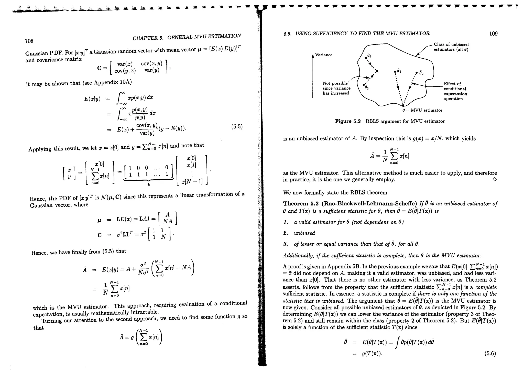
![110 CHAPTER 5. GENERAL MVU ESTIMATION
If T(x) is complete, there is but one function of T that is an unbiased estimator. Hence,
eis unique, independent of the jj we choose from the class shown in Figure 5.2. Every
jj maps into the same estimator e. Because the variance of emust be less than jj for
any jj within the class (property 3 of Theorem 5.2), we conclude that emust be the
MVU estimator. In summary, the MVU estimator can be found by taking any unbiased
estimator and carrying out the operations in (5.6). Alternatively, since there is only
one function of the sufficient statistic that leads to an unbiased estimator, we need only
find the unique 9 to make the sufficient statistic unbiased. For this latter approach we
found in Example 5.5 that g(2:::01 x[nJ) = 2:::01x[nJ/N.
The property of completeness depends on the PDF of x, which in turn determines
the PDF of the sufficient statistic. For many practical cases of interest it holds. In par-
ticular, for the exponential family of PDFs (see Problems 5.14 and 5.15) this condition
is satisfied. To validate that a sufficient statistic is complete is in general quite difficult,
and we refer the reader to the discussions in [Kendall and Stuart 1979J. A flavor for
the concept of completeness is provided by the next two examples.
Example 5.6 - Completeness of a Sufficient Statistic
For the estimation of A, the sufficient statistic 2:::01
x[nJ is complete or there is but
one function 9 for which E[g(2:::01 x[nJ)] = A. Suppose, however, that there exists
a second function h for which E[h(2:::~ x[nJ)] = A. Then, it would follow that with
T = 2:~:Ol x[nJ,
E [geT) - h(T)J = A - A = 0
or since T rv N(NA, N (12)
for all A
100 veT) ~exp [- N
1
2(T - NA)2] dT = 0
-00 2~N~ 2 (1
for all A
where veT) =geT) - h(T). Letting r =TIN and V'(T) =v(Nr), we have
100 vl(r)~exp[-2N2(A-r)2] dr=O
-00 2~ N(12 (1
for all A (5.7)
which may be recognized as the convolution of a function v'(r) with a Gaussian pulse
w(r) (see Figure 5.3). For the result to be zero for all A, v'(r) must be identically zero.
To see this recall that a signal is zero if and only if its Fourier transform is identically
zero, resulting in the condition
V'(f)W(f) = 0 for all f
where V'C!) = F{v'(r)} and W(f) is the Fourier transform of the Gaussian pulse in
(5.7). Since W(f) is also Gaussian and therefore positive for all f, we have that the
condition is satisfied if and only if V'(f) = 0 for all f. Hence, we must have that
v'(r) = 0 for all r. This implies that 9 = h or that the function 9 is unique. 0
r
5.5. USING SUFFICIENCY TO FIND THE MVU ESTIMATOR
Gaussian pulse, W(AI - r)
Choose Vi (r) to make
1:v'(r)w(A1-r)dr=O
r
Gaussian pulse, W(A2 - r)
r
(a) Integral equals zero
(b) Integral does not equal zero
Figure 5.3 Completeness condition for sufficient statistic (satisfied)
Example 5.1 - Incomplete Sufficient Statistic
Consider the estimation of A for the datum
x[OJ = A +w[OJ
111
where w[O) rvU[-! !) As ffi' t t t' " [) .
fu th [OJ .2' 2 . .u cien .s a IStrC IS x 0, bemg the only available data and
r ermore, x IS an unbIased estimator of A W, I d '
is.a viabl.e candidate for the MVU estimator. That
e
i~~::C~:~l~ e ~h~g(x[O]).= x[O)
stIll reqmres us to verify that it is a complete sufficient statisti~ t A: in~~ estrm~tor
example, we suppose that there exists another function h with the b' : preVIOUS
h(x[oP = A and attempt to prove that h = g. Again lettin veT) ~n (Ias)e property
examme the possible solutions for v of the equation g - 9 T - h(T), we
1:v(T)p(x; A) dx = 0 for all A.
For this problem, however, x = x[O) = T, so that
1:v(T)p(T; A) dT = 0 for all A.
But
p(T;A) = { ~ A-!<T<A+!
2 - - 2
otherwise
so that the condition reduces to
for all A.](https://image.slidesharecdn.com/fundamentalsofstatisticalsignalprocessing-estimationtheory-kay-230513154707-1f7652e0/75/Fundamentals-Of-Statistical-Signal-Processing-Estimation-Theory-Kay-pdf-61-2048.jpg)
![112
CHAPTER 5. GENERAL MVU ESTIMATION
f_:v(T)p(T; AI) dT =0
I:v(T)p(T; A2) dT = 0
(a) Integral equals zero
(b) Integral equals zero
Figure 5.4 Completeness condition for sufficient statistic (not satisfied) )
The nonzero function v(T) = sin 21fT will satisfy this condition as illustrated in Fig-
ure 5.4. Hence a solution is
v(T) = g(T) - h(T) = sin 21fT
or
h(T) =T - sin 21fT.
As a result, the estimator
A=x[O] - sin 21fx[0]
is also based on the sufficient statistic and is unbiased for A. Having found at least
one other unbiased estimator that is also a function of the sufficient statistic, we may
conclude that the sufficient statistic is not complete. The RBLS theorem no longer
holds, and it is not possible to assert that A= x[O] is the MVU estimator. 0
To summarize the completeness condition, we say that a sufficient statistic is complete
if the condition
I:v(T)p(T; (}) dT =0 for all () (5.8)
is satisfied only by the zero junction or by v(T) =0 for all T.
At this point it is worthwhile to review our results and then apply them to an
estimation problem for which we do not know the MVU estimator. The procedure is
as follows (see also Figure 5.5):
1. Find a single sufficient statistic for (), that is, T(x), by using the Neyman-Fisher
factorization theorem.
2. Determine if the sufficient statistic is complete and, if so, proceed; if not, this
approach cannot be used.
5.5. USING SUFFICIENCY TO FIND THE MVU ESTIMATOR
Use Neyman-Fisher factorization
theorem to find sufficient
statistic
T(x)
Determine if T(x) is complete
See (5.8)
F'ind function of T(x) that
is unbiased
113
{j = g(T(x)) = MVU estimator
Figure 5.5 Procedure for finding
MVU estimator (scalar parameter)
3. Fgin(;(:)f)un~~OenMgVOuf thte. suffici~nt stati~tic that yields an unbiased estimator 8 =
. es Imator IS then ().
As an alternative implementation of step 3 we may
3.' Evaluate 8 = E(8IT(x)) h ()- . .
, were IS any unbIased estimator.
However, in practice the conditional . . .
next example illustrates the overall ;::~t::~~n evaluatIOn IS usually too tedious. The
Example 5.8 - Mean of Uniform Noise
We observe the data
x[n] = w[n] n = 0,1, ... , N - 1
where w[n] is lID noise with PDF UfO ;3] for;3 .
for the mean () = /3/2 Our initial ap' h (0: We Wish to find the MVU estimator
and hence MVU esti~ator cannot ev~~o~c t ~ usmg t~e CRLB for finding an efficient
PDF does not satisfy the required regul:it;Ied ~.~.thiS (prOblem. This is because the
estimator of () is the sample mean or con 1 IOns see Problem 3.1). A natural
_ 1 N-I
()= N L x[n].
n=O
The sample mean is easily shown to be unbiased and to ha .
ve varIance
var(8) =
1
Nvar(x[n))
;32
12N'
(5.9)](https://image.slidesharecdn.com/fundamentalsofstatisticalsignalprocessing-estimationtheory-kay-230513154707-1f7652e0/75/Fundamentals-Of-Statistical-Signal-Processing-Estimation-Theory-Kay-pdf-62-2048.jpg)
![114 CHAPTER 5. GENERAL MVU ESTIMATION
To determine if the sample mean is the MVU estimator for this problem we will follow
the procedure outlined in Figure 5.5. Define the unit step function as
Then,
u(x) = {
1 for x > 0
o for x < O.
1
p(x[nJ; 9) = /3 [u(x[n]) - u(x[nJ - ,B)J
where,B = 29, and therefore the PDF of the data is
1 N-l
p(x; 9) = N II [u(x[nJ) - u(x[nJ - ,B)J .
,B n=O
This PDF will be nonzero only if 0 < x[nJ < ,B for all x[nJ, so that
{
~ 0 < x[nJ < ,B
p(x; 9) = ,BON
otherwise.
n = 0, 1, ... ,N - 1
Alternatively, we can write
so that
p(x;9) = {,Bo~ maxx[nJ <,B, minx[nJ > 0
otherwise
p(x; 9) = pu(,B - max x[nJ),:':n~.
.., ~
g(T(x),9) h(x)
By the Neyman-Fisher factorization theorem T(x) = maxx[nJ is a sufficient statistic
for 9. Furthermore, it can be shown that the sufficient statistic is complete. We omit
the proof.
Next we need to determine a function of the sufficient statistic to make it unbiased.
To do so requires us to determine the expected value of T = maxx[nJ. The statistic T
is known as an order statistic. Its PDF is now derived. Evaluating first the cumulative
distribution function
Pr{T::; 0 Pr{x[OJ ::; ~,x[lJ ::;~, ... ,x[N -lJ ::; 0
N-l
= II Pr{x[nJ ::;~}
n=O
••••••••••••••• IIIIIII ••••• 1
5.5. USING SUFFICIENCY TO FIND THE MVU ESTIMATOR
since the random variables are IID. The PDF follows as
dPr{T < 0
~
NPr{x[nJ ::; ON-l dPr{xtJ ::; O.
But dPr{x[nJ ::; O/~ is the PDF of x[nJ or
Po!o! «;0) ~ { ~ otherwise.
Integrating, we obtain
which finally yields
We now have
E(T) I:~PT(~) d~
ri3
(~)N-l 1
10 ~N /3 /3 ~
N
= N + 1,B
~9.
N+1
115
To make this unbiased we let {j = [(N +1)/2NJT, so that finally the MVU estimator is
. N+1
9 = 2N maxx[nJ.
Somewhat contrary to intuition, the sample mean is not the MVU estimator ofthe mean
for uniformly distributed noise! It is of interest to compare the minimum variance to
that of the sample mean estimator variance. Noting that
. (N+1)2
var(9) = 2N var(T)](https://image.slidesharecdn.com/fundamentalsofstatisticalsignalprocessing-estimationtheory-kay-230513154707-1f7652e0/75/Fundamentals-Of-Statistical-Signal-Processing-Estimation-Theory-Kay-pdf-63-2048.jpg)
![• • • • • • • • • • • • • • • • • ~ • • • - ~ * ~ ~ • • •
116 CHAPTER 5. GENERAL MVU ESTIMATION
and
var(T)
rf3
2N~N-l _ (-.!!L)2
Jo ~ (3N d{ N + 1
N(32
(N + 1)2(N + 2)
we have that the minimum variance is
A (32
var(O) = 4N(N + 2)'
(5.10)
This minimum variance is smaller than that of the sample mean estimator (see (5.9))
for N > 2 (for N = 1 the estimators are identical). The difference in the variances
is substantial for large N since the MVU estimator variance goes down as 1/N
2
as
compared to the l/N dependence for the sample mean estimator variance. ) 0
The success of the previous example hinges on being able to find a single sufficient
statistic. If this is not possible, then this approach cannot be employed. For instance,
recalling the phase estimation example (Example 5.4) we required two statistics, Tl (x)
and T2
(x). Theorem 5.2 may be extended to address this case. However, th~ M~U
estimator (assuming complete sufficient statisAtics or .E(g(Tb T2)) = O. for all ¢ Imphes
that 9 = 0) would need to be determined as ¢ = E(¢ITb T2), where ¢ is any unb~ased
estimator of the phase. Otherwise, we will need to guess at the form of the functIOn 9
that combines Tl and T2 into a single unbiased estimator for ¢ (see Problem 5.10). As
mentioned previously, the evaluation of the conditional expectation is difficult.
5.6 Extension to a Vector Parameter
We now extend our results to search for the MVU estimator for a p x 1 vector parameter
8. In this case we are seeking an unbiased vector estimator (each element is unbiased),
such that each element has minimum variance. Many of the results of the previous
sections extend naturally. In the vector case we may have more sufficient statistics
than the number of parameters (r > p), exactly the same number (r = p), or even
fewer sufficient statistics than parameters to be estimated (r < p). The cases of r > p
and r = p will be discussed in the following examples. For an example of r < p see
Problem 5.16. From our previous discussions a desirable situation would be to have
r = p. This would allow us to determine the MVU estimator by transf~rmi.ng t~e
sufficient statistics to be unbiased. The RBLS theorem may be extended to Justify thIS
approach for a vector parameter. Unfortunately, this approach is not always possibl~.
Before presenting some examples to illustrate these possibilities, extensions of the basiC
definitions and theorems will be given.
A vector statistic T (x) = [Tl (x) T2 (x) ... Tr (x)f is said to be sufficient for the
estimation of 8 if the PDF of the data conditioned on the statistic or p(xIT(x)j 8) does
not depend on 8. This is to say that p(xIT(x)j 8) = p(xIT(x)). In general, many such
• • • • • • • • • • • • • • • • • • • • • • • • • • • • 1
5.6. EXTENSION TO A VECTOR PARAMETER 117
T(x) exist (including the data x), so that we are interested in the minimal sufficient
statistic or the T of minimum dimension. To find the minimal sufficient statistic we can
again resort to the Neyman-Fisher factorization theorem which for the vector parameter
case is as follows.
Theorem 5.3 (Neyman-Fisher Factorization Theorem (Vector Parameter»
If we can factor the PDF p(Xj 8) as
p(Xj 8) = g(T(x), 8)h(x) (5.11)
where 9 is a function depending only on x through T(x), an r x 1 statistic, and also
on 8, and h is a function depending only on x, then T(x) is a sufficient statistic for 8.
Conversely, if T(x) is a sufficient statistic for 8, then the PDF can be factored as in
(5.11).
A proof can be found in [Kendall and Stuart 1979]. Note that there always exists a set
of sufficient statistics, the data set x itself being sufficient. However, it is the dimen-
sionality of the sufficient statistic that is in question, and that is what the factorization
theorem will tell us. Some examples now follow.
Example 5.9 - Sinusoidal Parameter Estimation
Assume that a sinusoidal signal is embedded in WGN
x[n] = A cos 21lJon + w[n] n = O,l, ... ,N - 1
where the amplitude A, frequency fo, and noise variance a 2
are unknown. The unknown
parameter vector is therefore 8 = [Afoa2
f. The PDF is
p(x;8,) = N exp --2 2)x[n]- A cos 211"fon)2 .
1 [1 N-l ]
(211"a2 ). 2a n=O
Expanding the exponent, we have
N-l N-l N-l N-l
L (x[n]- A cos 211"fon)2 = L x2[n]- 2A L x[n] cos 211"fon + A2 L cos2
211"fon.
n=O n=O n=O n=O
Now because of the term E::Ol x[n] cos 211"fon, where fo is unknown, we cannot reduce
the PDF to have the form expressed in (5.11). If, on the other hand, the frequency
were known, the unknown parameter vector would be 8 = [Aa2]T and the PDF could
be expressed as
p(x;8) =
1 [1 (N-l N-l N - l ) ]
(211"a2)~ exp - 2a2 ~ x
2
[n]- 2A ~ x[n] cos 211"fon + A2 ~ cos
2
211"fon . 1
, .. ~
g(T(x),8) h(x)](https://image.slidesharecdn.com/fundamentalsofstatisticalsignalprocessing-estimationtheory-kay-230513154707-1f7652e0/75/Fundamentals-Of-Statistical-Signal-Processing-Estimation-Theory-Kay-pdf-64-2048.jpg)
![~ ~ * ~ • • • ~ • ~ - - - - - - -
118
CHAPTER 5. GENERAL MVU ESTIMATION
where
l
%x[n] cos 27rfon 1
T(x) = N-l .
I>2[n]
n=O
Hence, T(x) is a sufficient statistic for A and a2
, but only if fa is known (see also
Problem 5.17). The next example continues this problem. 0
Example 5.10 _ DC Level in White Noise with Unknown Noise Power
If n = 0,1, ... , N - 1
x[n] = A +w[n]
where w[n] is WGN with variance a2 and the unknown parameters are A an(i a
2
, we
can use the results of the previous example to find a sufficient statistic of dimension
2. Letting the unknown vector parameter be 8 = [A a
2
f and letting fa = 0 in the
previous example, we have as our sufficient statistic
l
N-l 1
2:x[n]
T(x) = n=O •
N-l
2:x2[n]
n=O
Note that we had already observed that when a2
is known, L.~';:ol x[n] is a sufficient
statistic for A (see Example 5.2), and that when A is known (A = 0), L.~';:01 x
2
[n] is
a sufficient statistic for a2 (see Example 5.3). In this example, the same statistics are
jointly sufficient. This will not always be true, however. Since we have two parameters
to be estimated and we have found two sufficient statistics, we should be able to find
the MVU estimator for this example. 0
Before actually finding the MVU estimator for the previous example, we need to state
the RBLS theorem for vector parameters.
Theorem 5.4 (Rao-Blackwell-Lehmann-Scheffe (Vector Parameter» If () is
an unbiased estimator of 8 and T(8) is an r x 1 sufficient statistic for 8, then fJ =
E«(}T(x» is
1. a valid estimator for 8 (not dependent on 8)
.2. unbiased
3. of lesser or equal variance than that of () (each element of fJ has lesser or equal
variance)
y~-------~--------- ------
5.6. EXTENSION TO A VECTOR PARAMETER 119
Additionally, if the sufficient statistic is complete, then fJ is the MVU estimator.
In th~ vector parameter case completeness means that for veT)
functlOn of T, if ' an arbitrary r x 1
E(v(T» = Jv(T)p(T; 8) dT = 0
then it must be true that
veT) = 0 for aU T.
for aU 8 (5.12)
As before, this can be difficult to verify Al
estimator directly from T(x) without h '. t
SO
, t~ be able. to determine the MVU
the sufficient statistic should be equal tV~~g d~ eva ~ate E (8T(x)), the dimension of
r =p. If this is satisfied, then we need o~IY ~n~~~nslOd~ of t~e un
Ikfnow~ parameter or
'jr ImenSlOna unctlOn g such that
E(g(T» = 8
assuming that T is a complete sufficient statistic W 'U .
tinuing Example 5.10. . e I ustrate thiS approach by con-
n nown Olse Power (continued)
Example 5.11 - DC Level in WGN with U k N .
We first need to find the mean of the sufficient statistic
N-I
2:x[n]
n=O
Taking the expected value produces
E(T(x»= [ NA ]_[ NA ]
NE(x2[n]) - N(a2+A2) .
Clearly, we could remove the bias of the first com f . . .
by N. However, this would not help th d ponent 0 T(x) by dlVldmg the statistic
T
2
(x) _ "N-l x2
[n] t' t h e secon component. It should be obvious that
- L.m=O es ima es t e second t d .
we transform T(x) as momen an not the variance as desired. If
g(T(x»](https://image.slidesharecdn.com/fundamentalsofstatisticalsignalprocessing-estimationtheory-kay-230513154707-1f7652e0/75/Fundamentals-Of-Statistical-Signal-Processing-Estimation-Theory-Kay-pdf-65-2048.jpg)
![120
CHAPTER 5. GENERAL MVU ESTIMATION
then
E(x) = A
and
E (~ ~ x2[n] - X2) = a
2
+ A2 - E(x
2
).
But we know that x ~ N (A, a2
/ N), so that
and we have that
(
1 N-l ) 1 N - 1 2
E N~x2[n]-x2 =a2(1-N)=~a.
If we multiply this statistic by N/ (N - 1), it will then be unbiased for a
2
• Finally, the
appropriate transformation is
g(T(x)) = [
1fTl(x) ]
N~l [T2 (x) - N(1fTl(x))2]
=
[ NO' [~x:[n[-Nx'll
However, since
N-l
L(x[n]- x)2
n=O
N-l N-l
L x2[n]- 2 L x[n]x + Nx
2
n=O n=O
N-l
L x2
[n]- Nx
2
,
n=O
this may be written as
[
Xl
{j = 1 N-l
-- L (x[n] - x?
N-1 n=O
which is the MVU estimator of 6 = [Aa2
JT. The normalizing f~tor ~f l/~N -:-1) for;2
(the sample variance) is due to the one degree of freedom lost m estlmatmg the mean~
In this example {j is not efficient. It can be shown [Hoel, Port, and Stone 1971] that x
5.6. EXTENSION TO A VECTOR PARAMETER 121
and ;2 are independent and that
Hence, the covariance matrix is
CIi = [~ ~]
o N-1
while the CRLB is (see Example 3.6)
1-'(8) ~ [~ ,;,]
Thus, the MVU estimator could not have been obtained by examining the CRLB.
Finally, we should observe that if we had known beforehand or suspected that
the sample mean and sample variance were the MVU estimators, then we could have
reduced our work. The PDF
1 [1 N-l ]
p(x; 6) = (27ra2 ),¥- exp - 2a2 ~ (x[n]- A?
can be factored more directly by noting that
N-l N-l
L(x[n]-A? L (x[n] - x+ x - A)2
n=O n=O
N-l N-l
L (x[n]- X)2 + 2(x - A) L (x[n]- x) + N(x - A?
n=O
The middle term is zero, so that we have the factorization
1 {I [N-l ]}
p(x; 6) = (27ra2
),¥- exp - 2a2 ~ (x[n]- X)2 + N(x - A)2 . 1
, .. ' --..,....-
g(T'(x), 6) hex)
where
T'(x) = N-l .
[
Xl
~(x[n]-x?](https://image.slidesharecdn.com/fundamentalsofstatisticalsignalprocessing-estimationtheory-kay-230513154707-1f7652e0/75/Fundamentals-Of-Statistical-Signal-Processing-Estimation-Theory-Kay-pdf-66-2048.jpg)
![• ..........
122
CHAPTER 5. GENERAL MVU ESTIMATION
Dividing the second component by (N -1) would produce iJ. Of course T'(x) and T(x)
are related by a one-to-one transformation, illustrating once again that the sufficient
statistic is unique to within these transformations.
In asserting that iJ is the MVU estimator we have not verified the completeness
of the statistic. Completeness follows because the Gaussian PDF is a special case of
the vector exponential family of PDFs, which are known to be complete [Kendall and
Stuart 1979] (see Problem 5.14 for the definition of the scalar exponential family of
PDFs). 0
References
Hoel, P.G., s.c. Port, C.J. Stone, Introduction to Statistical Theory, Houghton Mifflin, Boston,
1971. )
Hoskins, R.F., Generalized Functions, J. Wiley, New York, 1979.
Kendall, Sir M., A. Stuart, The Advanced Theory of Statistics, Vol. 2, Macmillan, New York, 1979.
Papoulis, A., Probability, Random Variables, and Stochastic Processes, McGraw-Hill, New York,
1965.
Problems
5.1 For Example 5.3 prove that ~~:; x2
[n] is a sufficient statistic for a
2
by using the
definition that p(xl ~~:Ol x2 [n] =To; a2
) does not depend on a
2
• Hint: Note that
the PDF of s = ~~:Ol x2 [n]/a2 is a chi-squared distribution with N degrees of
freedom or
{
-=_I--:-:_exp (_~) /f-1
s > 0
p(s) = 2~r( If) 2
o s < O.
5.2 The IID observations x[n] for n =0,1, ... ,N - 1 have the Rayleigh PDF
p(x[n];a2 ) = { x;~] exp (O-~x:[~]) x[n] > 0
x[n] < O.
Find a sufficient statistic for a
2
.
5.3 The IID observations x[n] for n = 0,1, ... ,N - 1 have the exponential PDF
p(x[n]; >.) = { ,exp(~'x[n]) ~~~l ~ ~.
Find a sufficient statistic for ,.
5.4 The IID observations x[n] for n = 0,1, ... , N - 1 are distributed according to
.N(9,9), where 9 > O. Find a sufficient statistic for 9.
PROBLEMS 123
5.5 The IID observations x[~] for n = 0,1, ... ,N - 1 are distributed according to
U[-O,O], where 0 > O. Fmd a sufficient statistic for O.
5.6 If x[~] = A2+ w[n] for n = 0,1, ... , N - 1 are observed, where w[n] is WGN with
variance a , find the ~VU estimator for a2
assuming that A is known. You may
assume that the suffiCient statistic is complete. '
5.7 Consider the frequency estimation of a sinusoid embedded in WGN or
x[n] = cos 21l'fon +w[n] n = 0,1, ... ,N - 1
where w[n] is WGN of known variance a2
. Show that it is not possible to find a
sufficient statistic for the frequency fo.
5.8 In a similar fashion to Problem 5.7 consider the estimation of the damping constant
r for the data
x[n] = rn +w[n] n = 0, 1, ... , N - 1
where w[n] ~s WGN with known variance a 2
. Again show that a sufficient statistic
does not eXist for r.
5.9 Assume that x[n] is the result of a Bernoulli trial (a coin toss) with
Pr{x[n] = I} = 0
Pr{x[n] = O} = 1 - 0
and t~at .N IID observations have been made. Assuming the Neyman-Fisher
factOriZatIOn theor~m holds for discrete random variables, find a sufficient statistic
for O. Then, assummg completeness, find the MVU estimator of O.
5.10 For Example 5.4 the following estimator is proposed
J= - arctan [T2(X)]
T1 (x) .
Show that at high SNR or a2
-+ 0, for which
N-I
T1 (x) ~ L Acos(21l'fon +4»cos 21l'fon
n=O
N-1
T2 (x) ~ LAcos(21l'fon+4»sin21l'fon
n=O
the estimator sa~isfies J~ 4>. Use any approximations you deem appropriate. Is
the proposed estimator the MVU estimator?
5.11 Fo: Example 5.2 it is desired to estimate 0 = 2A +1 instead of A. Find the MVU
estimator.of 9. What if the parameter 0 = A3
is desired? Hint: Reparameterize
the PDF m terms of 0 and use the standard approach.](https://image.slidesharecdn.com/fundamentalsofstatisticalsignalprocessing-estimationtheory-kay-230513154707-1f7652e0/75/Fundamentals-Of-Statistical-Signal-Processing-Estimation-Theory-Kay-pdf-67-2048.jpg)
![124
CHAPTER 5. GENERAL MVU ESTIMATION
5.12 This problem examines the idea that sufficient statistics are Uniq~ehtohwithiffin ~net
to-one transformations. Once again, consider Example 5.2 but Wit t e su clen
statistics
N-l
Tl(X) L x[n]
n=O
Find functions gl and g2 so that the unbiased condition is satisfied or
E[gl (Tl (x))] = A
E[g2(T2 (x))] = A
and hence the MVU estimator. Is the transformation from Tl to T2 one-to-one?
What would happen if the statistic T3(X) = (l:~:OI x[n])2 were considered? Could
you find a function g3 to satisfy the unbiased constraint?
5.13 In this problem we derive the MVU estimator for an example .that we have not
encountered previously. If N IID observations are made accordmg to the PDF
( [ ]
.B) _ { exp[-(x[n]- B)] x[n] > B
P x n , - 0 x[n] < B,
find the MVU estimator for B. Note that B represents the minimum value that
x[n] may attain. Assume that the sufficient statistic is complete.
5.14 For the random variable x consider the PDF
p(x; B) = exp [A(B)B(x) + C(x) + D(B)].
A PDF of this type is said to belong to the scalar exponential far:"ily of PDFs.
Many useful properties are associated with this family, and in particular, that of
sufficient statistics, which is explored in this and the next problem. Show that
the following PDFs are within this class.
a. Gaussian
h. Rayleigh
c. Exponential
where). > O.
x>O
x <0.
••..........•.....•....•....,
PROBLEMS 125
5.15 If we observe x[n] for n = 0, 1, ... ,N - 1, which are IID and whose PDF belongs
to the exponential family of PDFs, show that
N-l
T(x) = L B(x[n])
n=O
is a sufficient statistic for B. Next apply this result to determine the sufficient
statistic for the Gaussian, Rayleigh, and exponential PDFs in Problem 5.14. Fi-
nally, assuming that the sufficient statistics are complete, find the MVU estimator
in each case (if possible). (You may want to compare your results to Example 5.2
and Problems 5.2 and 5.3, respectively.)
5.16 In this problem an example is given where there are fewer sufficient statistics
than parameters to be estimated [Kendall and Stuart 1979]. Assume that x[n] for
n = 0, 1, ... ,N - 1 are observed, where x '" N(I', C) and
NJ.L
o
o
o
C = [
N - 1+(J2 -1T ]
-1 I '
The covariance matrix C has the dimensions
[
Ix 1 1 x (N - 1) ]
(N - 1) x 1 (N - 1) x (N - 1) .
Show that with 8 = [J.L (J2JT
1 {I [N2 N - l ] }
p(x; 8) = -----;y- exp -- -2 (x - J.L)2 + L x2[n] .
(271") 2 (J 2 (J n=l
What are the sufficient statistics for 8? Hint: You will need to find the inverse
and determinant of a partitioned matrix and to use Woodbury's identity.
5.17 Consider a sinusoid of known frequency embedded in WGN or
x[n] = A cos 271"fon +w[n] n = 0, 1, ... , N - 1
where w[n] is WGN with variance (J2. Find the MVU estimator of
a. the amplitude A, assuming (J2 is known
h. the amplitude A and noise variance (J2.](https://image.slidesharecdn.com/fundamentalsofstatisticalsignalprocessing-estimationtheory-kay-230513154707-1f7652e0/75/Fundamentals-Of-Statistical-Signal-Processing-Estimation-Theory-Kay-pdf-68-2048.jpg)
![126
CHAPTER 5. GENERAL MVU ESTIMATION
You may assume that the sufficient statistics are complete. Hint: The results of
Examples 5.9 and 5.11 may prove helpful.
5.18 If x[n] for n = 0,1, ... ,N - 1 are observed, where. t~e samples are V
D and
distributed according to U[(:/t, 92], find a sufficient stat1st1c for 6 = [9192] •
5.19 Recall the linear model in Chapter 4 in which the data are modeled as
x=H6+w
where w ,...., N(o, 0'21) with 0'2 known. Find the MVU es~imator ~f ~ ~y using the
Neyman-Fisher and RBLS theorems. Assume the suffic1~nt st~t1st1C 1S complete.
Compare your result with that described in Chapter 4. Hmt: F1rst prove that the
following identity holds:
(x - H6)T(x - H6) = (x - H8f(x - H8) + (6 - 8)THTH(6 - 9)
where
Appendix 5A
Proof of Neyman-Fisher Factorization
Theorem (Scalar Parameter)
Consider the joint PDF p(x, T(x); 9). In evaluating this PDF it should be noted
that T(x) is functionally dependent on x. Hence, the joint PDF must be zero when
evaluated at x = XQ, T(x) = To, unless T(xo) = To. This is analogous to the situation
where we have two random variables x and y with x = y always. The joint PDF
p(x, y) is p(x)8(y - x), a line impulse in the two-dimensional plane, and is a degenerate
two-dimensional PDF. In our case we have p(x, T(x) = To; 9) = p(x; 9)8(T(x) - To),
which we will use in our proof. A second result that we will need is a shorthand way
of representing the PDF of a function of several random variables. If y = g(x), for x a
vector random variable, the PDF of y can be written as
p(y) = Jp(x)8(y - g(x)) dx. (5A.1)
Using properties of the Dirac delta function [Hoskins 1979], this can be shown to be
equivalent to the usual formula for transformation of random variables [Papoulis 1965].
If, for example, x is a scalar random variable, then
~( ()) ~ 8(x - Xi)
ay-gx =L..J d
;=1 I-..!!..I
dx x=x,
where {X1,X2,'" ,Xk} are all the solutions of y = g(x). Substituting this into (5A.1)
and evaluating produces the usual formula.
We begin by proving that T(x) is a sufficient statistic when the factorization holds.
p(xIT(x) = To; 9) =
=
127
p(x, T(x) = To; 9)
p(T(x) = To; 9)
p(x; 9)8(T(x) - To)
p(T(x) = To; 8) .](https://image.slidesharecdn.com/fundamentalsofstatisticalsignalprocessing-estimationtheory-kay-230513154707-1f7652e0/75/Fundamentals-Of-Statistical-Signal-Processing-Estimation-Theory-Kay-pdf-69-2048.jpg)
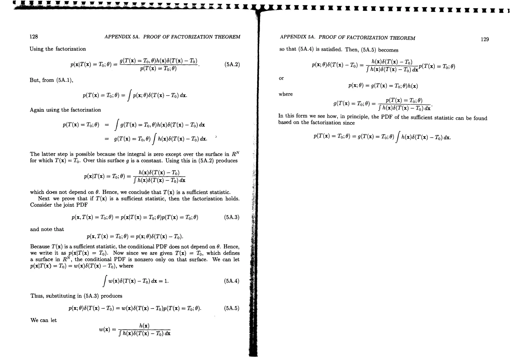
![Appendix 5B
Proof of
Rao-Blackwell-Lehmann-Scheffe
Theorem (Scalar Parameter)
To prove (1) of Theorem 5.2, that 0is a valid estimator of 8 (not a function of 8),
note that
o = E(8IT (x))
J8(x)p(xIT(x); 8) dx. (5B.1)
By the definition of a sufficient statistic, p(xIT(x); 8) does not depend on 8 but.only
on x and T(x). Therefore, after the integration is performed over x, the result WIll be
solely a function of T ~nd therefore of x only. • . .
To prove (2), that 8 is unbiased, we use (5B.1) and the fact that 8 IS a functIOn of
T only.
E(O) JJ8(x)p(xIT(x); 8) dxp(T(x); 8) dT
= J8(x) Jp(xIT(x); 8)p(T(x); 8) dT dx
J8(x)p(x; 8) dx
E(8).
But 8 is unbiased by assumption, and therefore
E(O) = E(8) = 8.
To prove (3), that
var(0) ~ var(8)
130
•..........................,
APPENDIX 5B. PROOF OF RBLS THEOREM 131
we have
var(8) E [(8 - E(8))2]
E [(8 - 0+0_ 8)2]
E[(8 - O?] +2E[(8 - 0)(0 - 8)] + E[(O - 8?].
The cross-term in the above expression, E[(O - 0)(0 - 8)], is now shown to be zero. We
know that 0is solely a function of T. Thus, the expectation of the cross-term is with
respect to the joint PDF of T and 8 or
But
and also
EOIT[8 - 0] = EOIT(8IT) - 0= 0- 0= O.
Thus, we have the desired result
var(8) E[(O - 0)2] +var(O)
~ var(O).
Finally, that 0is the MVU estimator if it is complete follows from the discussion given
in Section 5.5.](https://image.slidesharecdn.com/fundamentalsofstatisticalsignalprocessing-estimationtheory-kay-230513154707-1f7652e0/75/Fundamentals-Of-Statistical-Signal-Processing-Estimation-Theory-Kay-pdf-71-2048.jpg)
![134 CHAPTER 6. BEST LINEAR UNBIASED ESTIMATORS
6.3 Definition of the BLUE
We observe the data set {x[O] ,x[l], ... , x[N - 1]} whose PDF p(x; (J) depends on an
unknown parameter (J. The BLUE restricts the estimator to be linear in the data or
N-l
{) = L anx[n] (6.1)
n=O
where the an's are constants yet to be determined. (See also Problem 6.6 for a similar
definition except for the addition of a constant.) Depending on the an's chosen, we
may generate a large number of different estimators of (J. However, the best estimator
or BLUE is defined to be the one that is unbiased and has minimum variance. Before
determining the an's that yield the BLUE, some comments about the optimality of
the BLUE are in order. Since we are restricting the class of estimators to be linear,
the BLUE will be optimal (that is to say, the MVU estimator) only when the MVU
estimator turns out to be linear. For example, for the problem of estimating the value
of a DC level in WGN (see Example 3.3) the MVU estimator is the sample mean
A N-l 1
(J = x = L Nx[n]
n=O
which is clearly linear in the data. Hence, if we restrict our attention to only linear
estimators, then we will lose nothing since the MVU estimator is within this class.
Figure 6.1a depicts this idea. On the other hand, for the problem of estimating the
mean of uniformly distributed noise'(see Example 5.8), the MVU estimator was found
to be
which is nonlinear in the data. If we restrict our estimator to be linear, then the BLUE
is the sample mean, as we will see shortly. The BLUE for this problem is suboptimal,
as illustrated in Figure 6.1b. As further shown in Example 5.8, the difference in per-
formance is substantial. Unfortunately, without knowledge of the PDF there is no way
to determine the loss in performance by resorting to a BLUE.
Finally, for some estimation problems the use of a BLUE can be totally inappropri-
ate. Consider the estimation of the power of WGN. It is easily shown that the MVU
estimator is (see Example 3.6)
which is nonlinear in the data. If we force the estimator to be linear as per (6.1), so
that
N-l
;2 = L anx[n],
n=O
6.3. DEFINITION OF THE BLUE
(a)
mal
Linear
estimators
All unbiased
estimators
DC level in WGN; BLUE is opti·
All unbiased
• N+l
• (} = """"2N maxx[nJ
=MVU
(b) Mean of uniform noise; BLUE is
suboptimal
Figure 6.1 Optimality of BLUE
the expected value of the estimator becomes
N-l
E(;2) = L anE(x[n]) = 0
n=O
135
sinc~ E(x[n]) = 0 for all n. Thus, we cannot even find a single linear estimator that is
unb1a.:'ed, let alone one that has minimum variance. Although the BLUE is unsuitable
f~r thIS p~oblem, a BLUE utilizing the transformed data y[n] = x2[n] would produce a
VIable estImator since for
N-l N-l
;2 = L any[n] = L anx2[n]
n=O n=O
the unbiased constraint yields
N-l
E(;2) = L anu2 = u2.
n=O
There are many values of the an'S that could satisfy this constraint. Can you guess
w~at the an's should.be to yield the BLUE? (See also Problem 6.5 for an example of
thIS dat~ transformatIOn approach.) Hence, with enough ingenuity the BLUE may still
be used If the data are first transformed suitably.](https://image.slidesharecdn.com/fundamentalsofstatisticalsignalprocessing-estimationtheory-kay-230513154707-1f7652e0/75/Fundamentals-Of-Statistical-Signal-Processing-Estimation-Theory-Kay-pdf-73-2048.jpg)
![:IIII~IIII ••••••••••••••••• _ •
136 CHAPTER 6. BEST LINEAR UNBIASED ESTIMATORS
6.4 Finding the BLDE
To determine the BLUE we constrain 8 to be linear and unbiased and then find the
an's to minimize the variance. The unbiased constraint, is from (6.1),
N-I
E(8) = L anE(x[n]) = (J.
n=O
The variance of 8 is
[(
N-I (N-I)) 2]
var(8) = E ~ anx[n]- E ~ anx[n] .
But by using (6.2) and letting a = lao al ... aN-If we have
var(8) E [(aTx - aTE(x))2]
E[(aT(x-E(x))n
E [aT (x - E(x))(x - E(X))Ta]
aTCa.
(6.2)
(6.3)
The vector a of weights is found by minimizing (6.3) subject to the constraint of (6.2).
Before proceeding we need to assume some form for E(x[n]). In order to satisfy the
unbiased constraint, E(x[n]) must be linear in (J or
E(x[n]) = s[n](J (6.4)
where the s[nl's are known. Otherwise, it may be impossible to satisfy the constraint.
As an example, if E(x[n]) = cos(J, then the unbiased constraint is L,~':OI an cos(J = (J
for all (J. Clearly, there do not exist an's that will satisfy the unbiased constraint. Note
that if we write x[n] as
x[n] = E(x[n]) + [x[n] - E(x[n])]
then by viewing x[n] - E(x[n]) as noise or w[n] we have
x[n] =(Js[n] +w[n].
The assumption of (6.4) means that the BLUE is applicable to amplitude estimation of
known signals in noise. To generalize its use we require a nonlinear transformation of
the data as already described.
With the assumption given by (6.4) we now summarize the estimation problem. To
find the BLUE we need to minimize the variance
var(8) = aTCa
.-.---------------.-........,
6.4. FINDING THE BLUE
137
subject to the unbiased constraint, which from (6.2) and (6.4) becomes
N-I
L anE(x[n]) = (J
n=O
N-I
L ans[n](J (J
n=O
N-I
L ans[n] 1
n=O
or
aTs = 1
where s = [s[o] s[I] ... s[N -IW. The solution to this minimization problem is derived
in Appendix 6A as
so that the BLUE is
and has minimum variance
C-Is
Ilopt = STC-IS
. 1
var((J) = STC-IS.
Note from (6.4) that since E(x) = (Js, the BLUE is unbiased
E(8)
STC-I E(x)
STC-IS
STC-I(JS
STC-IS
(J.
(6.5)
(6.6)
Also, as we asserted earlier, to determine the BLUE we only require knowledge only of
1. s or the scaled mean
2. C, the covariance
or the first two moments but not the entire PDF. Some examples now follow.
Example 6.1 - DC Level in White Noise
If we observe
x[n] = A +w[n] n = 0, 1, ... , N - 1
where w[n] is white noise with variance a2 (and of unspecified PDF), then the problem
is to estimate A. Since w[n] is not necessarily Gaussian, the noise samples may be](https://image.slidesharecdn.com/fundamentalsofstatisticalsignalprocessing-estimationtheory-kay-230513154707-1f7652e0/75/Fundamentals-Of-Statistical-Signal-Processing-Estimation-Theory-Kay-pdf-74-2048.jpg)
![~.tl.'." 1, +; ; ; 't I :; :: I, ,,;; A I ,I. .I. .I. I I .I. JI JI • Ii •
CHAPTER 6. BEST
LINEAR UNBIASED ESTIMATORS
138 re uncorrelated. Because E(xlnJ) = A, we
statistically dependent
l
eJv~1t~~~g;h:~e~~r: s =1. From (6.5) the BLUE is
have from (6.4) that s n -
A. =
1
IT -Ix
a2
1
IT_Il
a2
N-l
= ~ LxlnJ=x
n:::;O
and has minimum variance, from (6.6),
var(A.)
a2
N' d"
n is the BL UE independent of the PDF ?f the data. In ad ItlO~
Hence, the sample me~. h MVU estimator for Gaussian nOlse.
as already discussed, It IS t e
1
62 DC Level in Uncorrelated Noise
ExaxnP e . - E I
. h (lnJ) - a2 and repeat xamp e
Now let wlnJ be z~ol me~f~:~o~~;)t::~ot~~6)lt var w - n
6.1. As before, s - , an
lTC-IX
A.= ~
1
var(A.) = }Tc-li'
The covariance matrix is
o 1
o
. ,
ai-l
and its inverse is 1
0
a6 1
0
ai
C-1
=
o
o
0 0
•••........................,
6.5. EXTENSION TO A VECTOR PARAMETER
Therefore,
var(A.)
~ x[n]
L a2
n=O n
N-l 1
L a2
n=O n
1
N-l 1 .
L a2
n=O n
139
(6.7)
(6.8)
The BLUE weights those samples most heavily with smallest variances in an attempt
to equalize the noise contribution from each sample. The denominator in (6.7) is the
scale factor needed to make the estimator unbiased. See also Problem' 6.2 for some
further results. 0
In general, the presence of C-1
in the BLUE acts to prewhiten the data prior to
averaging. This was previously encountered in Example 4.4 which discussed estimation
of a DC level in colored Gaussian noise. Also, in that example the identical estimator
for A was obtained. Because of the Gaussian noise assumption, however, the estimator
could be said to be efficient and hence MVU. It is not just coincidental that the MVU
estimator for Gaussian noise and the BLUE are identical for this problem. This is a
general result which says that for estimation of the parameters of a linear model (see
Chapter 4) the BLUE is identical to the MVU estimator for Gaussian noise. We will
say more about this in the next section.
6.5 Extension to a Vector Parameter
If the parameter to be estimated is a p x 1 vector parameter, then for the estimator to
be linear in the data we require
N-l
Oi = L a;nx[n] i = 1,2, ... ,p (6.9)
n=O
where the ain'S are weighting coefficients. In matrix form this is
where A is a p x N matrix. In order for (j to be unbiased we require
N-l
E(Oi) = L ainE(x[n]) = (Ji i = 1,2, ... ,p (6.10)
n=O](https://image.slidesharecdn.com/fundamentalsofstatisticalsignalprocessing-estimationtheory-kay-230513154707-1f7652e0/75/Fundamentals-Of-Statistical-Signal-Processing-Estimation-Theory-Kay-pdf-75-2048.jpg)
![• 'I!! I, J,; 11,,:'1 ,II.I. .. .I.I.': XIIII I I .. I -...~_I" ••••••••••••••••••••• """" I
140
CHAPTER 6. BEST LINEAR UNBIASED ESTIMATORS
or in matrix form
E(9) = AE(x) = fJ. (6.11)
Keep in mind that a linear estimator will be appropriate only for problems in which
the unbiased constraint can be satisfied. From (6.11) we must have that
E(x) = H9
for H a known N x p matrix. In the scalar parameter case (see (6.4))
E(x) =
[ :f~l 1
s[N:- 1] ()
~
H
(6.12)
so that (6.12) is truly the vector parameter generalization. Now, substitution of (6.12)
into (6.11) produces the unbiased constraint
AH=I. (6.13)
If we define a; = [aiO ail ... ai(N-Ilf, so that e
i = aTx, the unbiased constraint may be
rewritten for each ai by noting that
and letting 11; denote the ith column of H, so that
H = [hi h2 . .. hp].
With these definitions the unbiased constraint of (6.13) reduces to
i =1,2, ... ,p; j =1,2, ... ,p. (6.14)
Also, the variance is
var(ei) = arCa; (6.15)
using the results for the scalar case (see (6.3)). The BLUE for a ve~tor para~~te: is
found by minimizing (6.15) subject to the constraints of (6.1~), repeatIn~ the mInimiZa-
tion for each i. In Appendix 6B this minimization is carned out to Yield the BLUE
as (6.16)
and a covariance matrix of
(6.17)
6.6. SIGNAL PROCESSING EXAMPLE 141
The form of the BLUE is identical to the MVU estimator for the general linear model
(see (4.25)). This extends the observations of Examples 6.1 and 6.2. That this should
be the case follows from the definition of the general linear model
x = HfJ +w
where w '" N(O, C). With this model we are attempting to estimate fJ, where E(x) =
HfJ. This is exactly the assumption made in (6.12). But from (4.25) the MVU estimator
for Gaussian data is
9 = (HTC-1H)-IHTC-1X
which is clearly linear in x. Hence, restricting our estimator to be linear does not lead
to a suboptimal estimator since the MVU estimator is within the linear class. We may
conclude that if the data are truly Gaussian, then the BLUE is also the MVU estimator.
To summarize our discussions we now state the general BLUE for a vector parameter
of a general linear model. In the present context the general linear model does not
assume Gaussian noise. We refer to the data as having the general linear model form.
The following theorem is termed the Gauss-Markov theorem.
Theorem 6.1 (Gauss-Markov Theorem) If the data are of the general linear model
form
x = HfJ+w (6.18)
where H is a known N x p matrix, fJ is a p x 1 vector of parameters to be estimated, and
w is a N x 1 noise vector with zero mean and covariance C (the PDF of w is otherwise
arbitrary), then the BLUE of fJ is
(6.19)
and the minimum variance of e
i is
(6.20)
In addition, the covariance matrix of {} is
(6.21)
Some properties of BLUEs are given in Problems 6.12 and 6.13. Further examples
of the computation of BLUEs are given in Chapter 4.
6.6 Signal Processing Example
In the design of many signal processing systems we are given measurements that may
not correspond to the "raw data." For instance, in optical interferometry the input to
the system is light, and the output is the photon count as measured by a photodetector
[Chamberlain 1979J. The system is designed to mix the incoming light signal with a
delayed version of itself (through spatially separated mirrors and a nonlinear device).](https://image.slidesharecdn.com/fundamentalsofstatisticalsignalprocessing-estimationtheory-kay-230513154707-1f7652e0/75/Fundamentals-Of-Statistical-Signal-Processing-Estimation-Theory-Kay-pdf-76-2048.jpg)
![142
• Antenna 1
Aircraft
.~ ~
CHAPTER 6. BEST LINEAR UNBIASED ESTIMATORS
R3 ~~ - ~~. Antenna 3
• Antenna 2
ti = Time of received signal (emitted
by aircraft) at antenna i
Figure 6.2 Localization of aircraft by time difference
of arrival measurements
The data then is more nearly modeled as an autocorrelation function. The ~aw data,
that is, the light intensity, is unavailable. From the given information it is desired
to estimate the spectrum of the incoming light. To assume that the measurements
are Gaussian would probably be unrealistic. This is because if a random process is
Gaussian, then the autocorrelation data are certainly non-Gaussian [Anderson 1971].
Furthermore, the exact PDF is impossible to find in general, being mathematically
intractable. Such a situation lends itself to the use of the BLUE. A second example is
explored in some detail next.
Example 6.3 - Source Localization
A problem of considerable interest (especially to anyone who has traveled by airplane) is
that of determining the position of a source based on the emitted signal of the source. In
order to track the position of an aircraft we typically use several antennas. A common
method as shown in Figure 6.2 is to base our estimate on the time difference of arrival
(TDOA) measurements. In the figure the signal emitted by the aircraft is received at
the same time at all three antennas, so that tl = t2 = t3. The TDOA t2 - tl between
antennas 1 and 2 is zero, as is the TDOA t3 - t2 between antennas 2 and 3. Hence, we
may conclude that the ranges ~ to all three antennas are the same. The dashed line
between antennas 1 and 2 indicates the possible positions of the aircraft in order for
Rl = R2 , and likewise for the dashed line between antennas 2 and 3. The intersection
of these lines gives the aircraft position. In the more general situation for which the
TDOAs are not zero, the dashed lines become hyperbolas, the intersection again giving
the position. It is necessary to have at least three antennas for localization, and when
noise is present, it is desirable to have more.
We now examine the localization problem using estimation theory [Lee 1975]. To
do so we assume that N antennas have been placed at known locations and that the
time of arrival measurements ti for i = 0,1, ... ,N -1 are available. The problem is to
estimate the source position (x., Y.) as illustrated in Figure 6.3. The arrival times are
assumed to be corrupted by noise with zero mean and known covariance but otherwise
.. ------------------ • • • • • • • • c
6.6. SIGNAL PROCESSING EXAMPLE
Nominal position (xn, Yn)
Antenna
·0
•1
...
Figure 6.3 Source localization geometry
143
L x
unknown PDF. For a signal emitted by the source at time t - 1: th
are modeled by - 0, e measurements
, ti=To+R;jc+fi i=0,1, ... ,N-1 (6.22)
where
I the fi s are measurement noises and C denotes the propagation speed Th .
samp es are assumed to be zero mean with va . 2 d . e nOlse
th N, nance (j an uncorrelated with h
o er. 0 assumptions are made about the PDF 1th . 1:: eac
must relate the range from each antenna R~ t tOh e kno~se. 0 ?~oceed further we
L tt· h . . , 0 e un nown POSItIOn (J - [ ]T
e mg t e pOSItion of the ith antenna be (x~ .) h· h . - x. Y. .
have that "y, , W IC IS assumed to be known, we
Ri = Vex. -XiP + (y. -YiP. (6.23)
Substituting (6.23) into (6.22), we see that the model is nonlinear in the k
para~etlers x. and. ~.. To apply the Gauss-Markov theorem we will assumUenthnotwn
nomma Source pOSItIOn (x ) . ·1 bl T· . a a
th . . n, Yn IS aval a e. hIS nommal position which is I t
. e tr~e s?urce pOSItion, could have been obtained from revious m ' c ose 0
~ltu.a~lOn IS typical when the source is being tracked. He~ce to esti~as~r~~ents. Such a
P?SItlOn we require an estimate of (J = [(x. _ xn) (y _ )]'T _ [6 ~ e]T e new sour~e
FIgure 6.3. Denote the nominal ran es b R • Yn - x. Y. ,as shown m
R ( .d d . . g y ni· We use a first-order Taylor expansion of
,_consl ere as a two-dImenSIOnal function of x. and Y.) about the nominal .t.
x. - Xn,Y. =Yn POSI Ion
R·::::::R +~J.: Yn-Yi
, ni R. uX. + --6y.. (6.24)
n, Rni
See also ~hapte.r 8 for a more complete description of the linearization of a non!"
model. WIth thIS approximation we have upon substitution in (6.22) mear
t 1: + Rni Xn - Xi Y - y~
i = 0 - + ---6x + _n
_ _
, 6
C R ~C • R Y. + fi
n, niC
which is now linear in the unknown parameters 6x and 6y A
defined in Figure 6.3 • •. Iternatively, since as
COS eti](https://image.slidesharecdn.com/fundamentalsofstatisticalsignalprocessing-estimationtheory-kay-230513154707-1f7652e0/75/Fundamentals-Of-Statistical-Signal-Processing-Estimation-Theory-Kay-pdf-77-2048.jpg)
![144
CHAPTER 6. BEST LINEAR UNBIASED ESTIMATORS
sinoi,
the model simplifies to
Rn. COSOi sinoi
ti = To + -' + --8xs + --8ys +€i'
e c e
The term Rn./e is a known constant which can be incorporated into the measurement
by letting (see also Problem 6.6)
Hence, we have for our linear model
Rni
Ti=ti--'
C
COSOi sinoi
Ti = To + --8xs + --8ys + €i
C e
(6.25)
where the unknown parameters are To, 8x., 8ys' By assuming the time To when the
source emits a signal is unknown, we are bowing to practical considerations. Knowledge
of To would require accurate clock synchronization between the source and the receiver,
which for economic reasons is avoided. It is customary to consider time difference of
arrivals or TDOA measurements to eliminate To in (6.25). We generate the TDOAs as
6 T1 - TO
6 T2 - T1
~N-1 = TN-1 - TN-2'
Then, from (6.25) we have as our final linear model
~i = ~(COSOi - COSOi_1)8xs + ~(sinoi - sinoi_1)8ys + €i - €i-1
e c
(6.26)
for i = 1,2, ... ,N - 1. An alternative but equivalent approach is to use (6.25) and
estimate To as well as the source position. Now we have reduced the estimation problem
to that described by the Gauss-Markov theorem where
8 = [8xs 8Ys]T
cos 01 - cos 00 sin 01 - sin 00
1
1 [
cos 02 - cos 01 sin 02 - sin 01
H e :
COSON-1 - COSON-2 sinoN_1 - sinoN-2
w =
[
101 - 100 1
102 - 101
€N-1 ~€N-2 .
......................... . . . . . . . t
6.6. SIGNAL PROCESSING EXAMPLE 145
• Source
o 2
- d -~"_"f--- d _
Figure 6.4 Example of source lo-
calization geometry for line array
with minimum number of antennas
Th~ noise vector w is zero mean but is no longer composed of uncorrelated rando
vanables. To find the covariance matrix note that m
1
-1
o
o
1
o
o
o -1 flUJ
~-------~~------~.~
A E
~~~re A has dimension (N - 1) x N. Since the covariance matrix of e is 0'21, we have
C = E[AeeTAT] = O'
2 AAT.
From (6.19) the BLUE of the source position parameters is
iJ (HTC-1H)-1HTC-1e
[HT (AAT)-1H]-1HT (AAT)-1e (6.27)
and the minimum variance, is from (6.20),
var(Bi) = 0'2 [{HT(AAT)-1H} -1] ..
"
(6.28)
or the covariance matrix, is from (6.21),
H 1 [ - coso 1 - sino
e -coso -(1- sino)
A [~1 !1 ~].](https://image.slidesharecdn.com/fundamentalsofstatisticalsignalprocessing-estimationtheory-kay-230513154707-1f7652e0/75/Fundamentals-Of-Statistical-Signal-Processing-Estimation-Theory-Kay-pdf-78-2048.jpg)
![•
146
CHAPTER 6. BEST LINEAR UNBIASED ESTIMATORS
After substituting in (6.29) we have for the covariance matrix
o 1
3/2 .
(1- sina)2
For the best localization we would like a to be small. This is accomplished by making
the spacing between antennas d large, so that the baseline of the array, which is the
total length, is large. Note also that the localization accuracy is range dependent, with
the best accuracy for short ranges or for a small.
References
Anderson, T.W., The Statistical Analysis of Time Series, J. Wiley, New York, 1971.
Chamberlain, J., The Principles of Interferometric Spectroscopy, J. Wiley, New York, 1979.
Lee, H.B., "A Novel Procedure for Assessing the Accuracy of Hyperbolic Multilateration Systems,"
IEEE Trans. Aerosp. Electron. Syst., Vol. 11, pp. 2-15, Jan. 1975.
Problems
6.1 If x[n] = Arn +w[n] for n = 0,1, ... , N - 1, where A is an unknown parameter, r
is a known constant, and w[n] is zero mean white noise with variance 0-
2
, find the
BLUE of A and the minimum variance. Does the minimum variance approach
zero as N -+ oo?
6.2 In Example 6.2 let the noise variances be given by o-~ = n + 1 and examine what
happens to the variance of the BLUE as N -+ 00. Repeat for o-~ = (n + 1)2 and
explain your results.
6.3 Consider the estimation problem described in Example 6.2 but now assume that
the noise samples are correlated with the covariance matrix
1 P 0 0
P I
0
I P 0
e =0-
2 P I
0 0
I P
P 1
where Ipi < I and N, the dimension of the matrix, is assumed to be even. C is
a block-diagonal matrix and so is easily inverted (see (Appendix 1)). Find the
BLUE and its variance and interpret your results.
PROBLEMS 147
6.4 T;~;;served samples {x[O], x[I], ... , x[N - I]} are lID according to the following
a. Laplacian
1
p(x[n]; J-L) = 2exp[-Ix[n]- J-LI]
h. Gaussian
p(x[n]; J-L) = ~ exp [-~(x[n]- J-L)2] .
Fi~d the BLUE of the mean J-L in both cases. What can you say about the MVU
estImator for J-L?
6.5 T;~~bserved samples {x[O],x[I], ... ,x[N -I]} are lID according to the lognormal
p(x[n]; 0) = { ~x[n] exp [-~(lnx[n] - 0)2] x[n] > 0
o x[n] < O.
Prove that th.e mean i~ exp(O + 1/2) and therefore that the unbiased constraint
ca[nnot be satIsfied. Usmg the transformation of random variables approach with
y n] = lnx[n], find the BLUE for O.
6.6 In this probl~m we extend the scalar BLUE results. Assume that E(x[n]) = Os[n] +
/3, where 0 IS the unknown parameter to be estimated and /3 is a known constant.
The data ~ector x has covariance matrix e. We define a modified linear (actuall
affine) estImator for this problem as y
N-I
{} = L anx[n] + b.
n=O
Prove that the BLUE is given by
{} = sTe-l(x - /31)
sTe-Is
Also, find the minimum variance.
6.7 Assume that x[n] = As[n] + w[n] for n = 0 1 N - 1 b d h
fl
' " ... , are 0 serve ,were
w n IS ze.ro mean. noise wit~ covariance matrix e and s[n] is a known signal.
The amplItude. A IS to be estImated using a BLUE. Find the BLUE and discuss
w~a.t happen~ If s = [s[O] s[l] ... s[N - 1]JT is an eigenvector of e. Also find the
mmlmum varIance. '
6.8 eonti~uin~ Problem 6.7, we can always represent the signal vector s as a linear
c?mbmatlOn of the eigenvectors of e. This is because we can always find N
eIgenvectors that are linearly independent. Furthermore, it can be shown that](https://image.slidesharecdn.com/fundamentalsofstatisticalsignalprocessing-estimationtheory-kay-230513154707-1f7652e0/75/Fundamentals-Of-Statistical-Signal-Processing-Estimation-Theory-Kay-pdf-79-2048.jpg)
![148 CHAPTER 6. BEST LINEAR UNBIASED ESTIMATORS
these eigenvectors are orthonormal due to the symmetric nature of C. Hence, an
orthogonal representation of the signal is
N-l
s= L aiv;
i=O
where {vo, Vb ... , VN-d are the orthonormal eigenvectors of C. Prove that the
minimum variance of the BLUE is
A 1
var(A) = - -
N-l 2
La;
i=O Ai
where Ai is the eigenvalue of C corresponding to the eigenvector V;. Next show
that the signal energy £. = STS is given by ~;:~l aT. Finally, prove that if the
energy is constrained to be some value £'0, then the smallest possible> variance of
the BLUE is obtained by choosing the signal
S = CVrnin
where Vrnin is the eigenvector of C corresponding to the minimum eigenvalue and
c is chosen to satisfy the energy constraint £.0 = sTS = c2. Assume that the
eigenvalues of C are distinct. Explain why this result makes sense.
6.9 In an on-off keyed (OaK) communication system we transmit one of two signals
SO(t) = 0
to represent a binary 0 or
SI(t) = Acos271"/lt
to represent a binary 1. The amplitude A is assumed to be positive. To determine
which bit was transmitted we sample the received waveform to produce
x[n] = s;[n] +w[n] n = 0, 1, ... ,N - 1.
If a 0 was transmitted, we would have s;[n] = 0, and if a 1 was transmitted, we
would have s;[n] = Acos271"/ln (assuming a sampling rate of 1 sample/s). The
noise samples given by w[n] are used to model channel noise. A simple receiver
might estimate the sinusoidal amplitude A and decide a 1 was sent if A> 'Y, and
a 0 if A < 'Y. Hence, an equivalent problem is to estimate the amplitude A for
the received data
x[n] = Acos 21r/tn +w[n] n = 0, 1, ... , N - 1
where w[n] is zero mean noise with covariance matrix C = 0-
2
1. Find the BLUE
for this problem and interpret the resultant detector. Find the best frequency in
the range 0 $ /1 < 1/2 to use at the transmitter.
••••••••••••••••••• IIIIIIII.1
PROBLEMS
x[n] ~"---- A
Sample at
n=N-l
N-l
1i.(z) = L h[k]z-k
k=O
149
Figure 6.5 FIR filter estimator
for Problem 6.11
6.10 We continue Problem 6.9 by examining the question of signal selection for an
OaK system in the presence of colored noise. Let the noise w[n] be a zero mean
WSS random process with ACF
k=O
k=l
k=2
k;::: 3.
Find the PSD and plot it for frequencies 0 $ / $ 1/2. As in the previous
problem, find the frequency which yields the smallest value of the BLUE variance
for N = 50. Explain your results. Hint: You will need a computer to do this.
6.11 Consider the problem of estimating a DC level in WSS noise or given
x[n] = A +w[n] n = 0, 1, ... ,N - 1
where w[n] is a zero mean WSS random process with ACF Tww[k], estimate A. It
is proposed to estimate A by using the output of the FIR filter shown in Figure 6.5
at time n = N - 1. Note that the estimator is given by
N-l
A= L h[k]x[N - 1 - k].
k=O
The input x[n] is assumed to be zero for n < O. To obtain a good estimator we
wish to have the filter pass the DC signal A but block the noise w[n]. Hence,
we choose H(exp(jO)) = 1 as a constraint and minimize the noise power at the
output at time n = N - 1 by our choice of the FIR filter coefficients h[k]. Find
the optimal filter coefficients and the minimum noise power at the output of the
optimal filter. Explain your results.
6.12 Prove that the BLUE commutes over linear (actually affine) transformations of
9. Thus, if we wish to estimate
a=B9+b
where B is a known p x p invertible matrix and b is a known p x 1 vector, prove
that the BLUE is given by](https://image.slidesharecdn.com/fundamentalsofstatisticalsignalprocessing-estimationtheory-kay-230513154707-1f7652e0/75/Fundamentals-Of-Statistical-Signal-Processing-Estimation-Theory-Kay-pdf-80-2048.jpg)
![",.44,1 A A 4' .1,.&,.1. .1...1. .... ~ ;a . . . . . . . . . . . . .
150 CHAPTER 6. BEST LINEAR UNBIASED ESTIMATORS
where 6 is the BLUE for 8. Assume that x = H8 + w, where E(w) = 0 and
E(wwT ) =C. Hint: Replace 8 in the data model by o.
6.13 In this problem it is shown that the BLUE is identical to the weighted least squares
estimator to be discussed in Chapter 8. In particular, the weighted least squares
estimator is found by minimizing the criterion
J = (x - H8?C-I
(x - H8).
Prove that the 8 that minimizes J is the BLUE.
6.14 A noise process is composed of IID zero mean random variables with PDF
p(w[n]) = ~exp [_~ (w2~nl)] + _t_exp [_~ (w2[nl)]
J21f(1~ 2 ab J27raJ 2 aJ
where 0 < t < 1. Such a PDF is called a Gaussian mixture. It is used, to model
noise that is Gaussian with variance a1 for 100(1- €)% of the time and Gaussian
with variance aJ the remaining time. Typically, aJ » a1 and t «: 1, so that
the noise is predominately due to background noise with variance a1 but also
contains occasional high level events or interferences modeled as Gaussian noise
with variance aJ. Show that the variance of this PDF is
a2
= (1 - t )a1 + lOa;'
If {w2
[0], w2
[l), ... ,w2
(N -I]} is considered to be the data and a1, t are assumed
known, find the BLUE of aJ. Hint: Use the results of Problem 6.12.
6.15 For the general linear model
x=H8+s+w
where s is a known N x 1 vector and E(w) =0, E(wwT
) =C, find the BLUE.
6.16 In implementing the BLUE for the linear model described in Theorem 6.1, we
may unknowingly use the wrong covariance matrix to form the estimate
To examine the effect of this modeling error assume that we wish to estimate A
as in Example 6.2. Find the variance of this estimator and that of the BLUE for
the case where N = 2 and
C [~~ ]
C [~~].
Compare the variances for a -t 0, a = 1, and a -t 00.
Appendix 6A
Derivation of Scalar BLUE
To ~inimize ~r.(fJ) = aTCa subject to the constraint aTs = 1 we use the method of
Lagrangian multiplIers. The Lagrangian function J becomes
J = aTCa + A(aTs - 1).
Using (4.3), the gradient with respect to a is
8J
8a = 2Ca+ AS.
Setting this equal to the zero vector and solving produces
A -I
a= --C s
2 .
The Lagrangian multiplier A is found using the constraint equation as
T A T -I
a S= -"2S C s = 1
or
A 1
-"2 = STC-IS
so that the gradient is zero with the constraint satisfied for
C-IS
llopt = r-C
I .
S - s
The variance for this value of a is found from
a~PtC80Pt
STC-ICC-IS
(STC-Is)2
1
STC-IS'
151](https://image.slidesharecdn.com/fundamentalsofstatisticalsignalprocessing-estimationtheory-kay-230513154707-1f7652e0/75/Fundamentals-Of-Statistical-Signal-Processing-Estimation-Theory-Kay-pdf-81-2048.jpg)
![154 APPENDIX 6B. DERIVATION OF VECTOR BLUE
To find the vector of Lagrangian multipliers we use the constraint equations
or in combined form
j=I,2, ... ,p
o
hL 0
hT a; = 1
htl 0
hT
p
o
Letting ei denote the vector of all zeros except in the ith place, we have the constraint
equation
HTa; = ei.
Using (6B.l), the constraint equations become
HTa; = _~HTC-IH~i = ei
2
so that assuming invertibility of HTC-IH, the Lagrangian multiplier vector is
-~~i =(HTC-IH)-lei'
2
Using this in (6B.l) yields the final result
. = C-IH(HTC-IH)-le'
&ioPt t
and a corresponding variance of
aT Ca;
lopt opt
= e[(HTC-IH)-IHTC-ICC-IH(HTC-IH)-lei
= e[(HTC-IH)-lei'
(6B.2)
l"""'-
APPENDIX 6B. DERIVATION OF VECTOR BLUE
since [el e2 ... epf is the identity matrix. Also, the covariance matrix of iJ is
where
Thus,
8 - E(8) (HTC-IH)-IHTC-I(H8 + w) - E(8)
(HTC-IH)-IHTC-IW.
Cli = E[(HTC-IH)-IHTC-IWWTC-IH(HTC-IH)-I].
Since the covariance matrix of w is C, we have
Cli (HTC-IH)-IHTC-ICC-IH(HTC-IH)-1
(HTC-IH)-l
with the minimum variances given by the diagonal elements of Cli or
as previously derived.
155](https://image.slidesharecdn.com/fundamentalsofstatisticalsignalprocessing-estimationtheory-kay-230513154707-1f7652e0/75/Fundamentals-Of-Statistical-Signal-Processing-Estimation-Theory-Kay-pdf-83-2048.jpg)
![158 CHAPTER 7. MAXIMUM LIKELIHOOD ESTIMATION
function of the component., of 6. The asymptotic properties of the vector parameter
MLE are summarized in Theorem 7.3, and the invariance property in Theorem 7.4. For
the linear model the MLE achieves the CRLB for finite data records. The resultant
estimator is thus the usual MVU estimator as summarized in Theorem 7.5. Numerical
determination of the vector parameter MLE is based on the Newton-Raphson (7.48)
or scoring (7.50) approach. Another technique is the expectation-maximization (EM)
algorithm of (7.56) and (7.57), which is iterative in nature. Finally, for WSS Gaussian
random processes the MLE can be found approximately by maximizing the asymptotic
log-likelihood function of (7.60). This approach is computationally less intensive than
determination of the exact MLE.
7.3 An Example
As a rationale for why we might be interested in an approximately optimal estimator,
we now examine an estimation problem for which there is no obvious way to find
the MVU estimator. By resorting to the estimator based on the maximum likelihood
principle, termed the maximum likelihood estimator (MLE), we can obtain an estimator
that is approximately the MVU estimator. The nature of the approximation relies on
the property that the MLE is asymptotically (for large data records) efficient.
Example 7.1 - DC Level in White Gaussian Noise - Modified
Consider the observed data set
x[n] = A +w[n] n = 0, 1, ... ,N - 1
where A is an unknown level, which is assumed to be positive (A > 0), and w[n] is
WGN with 'Unknown variance A. This problem differs from our usual one (see Example
3.3) in that the unknown parameter A is reflected in the mean and the variance. In
searching for the MVU estimator of A we first determine the CRLB (see Chapter 3) to
see if it is satisfied with equality. The PDF is
p(x; A) = 1!i. exp [- 21A 'tl(x[n] - A)2] .
(27rA) 2 n=O
(7.1)
Taking the derivative of the log-likelihood function (the logarithm of the PDF consid-
ered as a function of A), we have
8lnp(x;A)
8A
N 1 N-l 1 N-l
= -- + - 2:)x[n] - A) + -2::(x[n] - A?
2A A n=O 2A2 n=O
J(A)(A - A).
It is certainly not obvious if the derivative of the log-likelihood function can be put in
the required form. It appears from a casual observation that it cannot, and therefore,
7.3. AN EXAMPLE 159
an efficient estimator does not exist. We can still determine the CRLB for this problem
to find that (see Problem 7.1)
, A2
var(A) ~ N(A + k)' (7.2)
We next try to find the MVU estimator by resorting to the theory of sufficient statistics
(see Chapter 5). Attempting to factor (7.1) into the form of (5.3), we note that
1 N-l 1 N-l
A 2::(x[n] - A)2 = A 2:: x
2
[n] - 2Nx + N A
n=O n=O
so that the PDF factors as
1 [ 1 ( 1 N-l )]
p(x; A) = N exp -- - 2:: x2
[n] + N A exp(Nx) .
(27rA)' 2 A n=O
~----------~y~--------~"~~~~'
g(%x2 [nJ,A) hex)
Based on the Neyman-Fisher factorization theorem a single sufficient statistic for A is
T(x) = ~~:Ol x2 [n]. The next step is to find a function of the sufficient statistic that
produces an unbiased estimator, assuming that T(x) is a complete sufficient statistic.
To do so we need to find a function 9 such that
Since
for all A > O.
NE[x2[nlJ
N [var(x[nJ) +E2(x[nJ)]
= N(A+A2)
it is not obvious how to choose g. We cannot simply scale the sufficient statistic to
make it unbiased as we did in Example 5.8.
A second approach would be to determine the conditional expectation E(AI ~~:Ol x2[nJ),
where A is any unbiased estimator. As an example, if we were to choose the unbiased
estimator A=x[O], then the MVU estimator would take the form
(7.3)](https://image.slidesharecdn.com/fundamentalsofstatisticalsignalprocessing-estimationtheory-kay-230513154707-1f7652e0/75/Fundamentals-Of-Statistical-Signal-Processing-Estimation-Theory-Kay-pdf-85-2048.jpg)
![160 CHAPTER 7. MAXIMUM LIKELIHOOD ESTIMATION
Unfortunately, the evaluation of the conditional expectation appears to be a formidable
task.
We have now exhausted our possible optimal approaches. This is not to say that
we could not propose some estimators. One possibility considers A to be the mean, so
that
A {x ifx>O
Al = 0 if x ~ 0
since we know that A > O. Another estimator considers A to be the variance, to yield
1 N-I
A2 = - - '" (x[nJ- AI)2
N-1 L.J
n=O
(see also Problem 7.2). However, these estimators cannot be claimed to be optimal in
any sense. o
Faced with our inability to find the MVU estimator we will propose an estimator that
is approximately optimal. We claim that for large data records or as N -+ 00, the
proposed estimator is efficient. This means that as N -+ 00
E(A) -+ A (7.4)
var(A) -+ CRLB, (7.5)
the CRLB being given by (7.2). An estimator A that satisfies (7.4) is said to be
asymptotically unbiased. If, in addition, the estimator satisfies (7.5), then it is said to
be asymptotically efficient. For finite data records, however, we can say nothing about
its optimality (see Problem 7.4). Better estimators may exist, but finding them may
not be easy!
Example 7.2 - DC Level in White Gaussian Noise - Modified (continued)
We propose the following estimator:
A 1
A=--+
2
This estimator is biased since
E(A) ~ E (-~ +
1 N-I 1
N L x2[nJ+ 4'
n=O
1N-I 1)
- Lx2[nJ+-
N n=O 4
(
1 N-I ) 1
E N ~x2[nJ +4
(7.6)
for all A
7.3. AN EXAMPLE
161
It is nonetheless a reasonable estimator in that as N -+ 00, we have by the law of large
numbers
1 N-I
N L x
2
[nJ-+ E(x2
[n]) = A + A2
n=O
and therefore from (7.6)
A-+A.
The estimator Ais said to be a consistent estimator (see Problems 7.5 and 7.6). To find
the mean and variance of A as N -+ 00 we use the statistical linearization argument
described in Section 3.6. For this example the PDF of 1:; 2:,:::01x2 [nJ will be concen-
trated about its mean, A + A2
, for large data records. This allows us to linearize the
function given in (7.6) that transforms 1:; 2:,:::01x2 [nJ into A. Let 9 be that function,
so that
A= g(u)
where u = 1:; 2:,:::01x2
[n], and therefore,
g(u)=-~+Ju+~
2 4'
Linearizing about Uo = E(u) = A + A2 , we have
g(u) ::::::: g(uo) + -- (u - uo)
d9(U)j
du U=Uo
or
1 [1 N-I ]
A::::::: A + A!! N ~ x
2
[nJ- (A + A2) .
It now follows that the asymptotic mean is
E(A) = A
(7.7)
so that A is asymptotically unbiased. Additionally, the asymptotic variance becomes,
from (7.7),
var(A) = (Ai!rvar [ ~ ~x
2
[nJ]
1
N(A ~ !)2var(x
2
[nJ).
But var(x
2
[n]) can be shown to be 4A3 + 2A2 (see Section 3.6), so that
A ~ 2 1
var(A) = N(A + V24A (A +"2)
A2](https://image.slidesharecdn.com/fundamentalsofstatisticalsignalprocessing-estimationtheory-kay-230513154707-1f7652e0/75/Fundamentals-Of-Statistical-Signal-Processing-Estimation-Theory-Kay-pdf-86-2048.jpg)
![162 CHAPTER 7. MAXIMUM LIKELIHOOD ESTIMATION
p(xo;9)
-+---..-L.-t-~-r--(}
Figure 7.1 Rationale for maxi-
mum likelihood estimator
which from (7.2) is the CRLB!
Summarizing our results, the proposed estimator given by (7.6) is asymptotically
unbiased and asymptotically achieves the CRLB. Hence, it is asymptotically efficient.
Furthermore, by the central limit theorem the random variable 1J L,~:Ol x2
[n] is Gaus-
sian as N -+ 00. Because A is a linear function of this Gaussian random variable for
large data records (as per (7.7)), it too will have a Gaussian PDF. <>
The proposed estimator is termed the MLE. How it was found is discussed in the next
section.
7.4 Finding the MLE
The MLE for a scalar parameter is defined to be the value of B that maximizes p Xj B
or x e, I.e., t e ue that maximizes t e likelihoo unction. The maximization is
performed over the allowable range of B. In the previous example this was A> O. Since
p(x; B) will also be a function of x, the maximization produces a 8that is a function of x.
The rationale for the MLE hinges on the observation that p(Xj B) dx gives the probability
of observing x in a small volume for a given B. In Figure 7.1 the PDF is evaluated for
x = Xo and then plotted versus B. The value of p(x = Xo; B) dx for each B tells us the
probability of observing x in the region in RN centered around Xo with volume dx,
assuming the given value of B. If x = Xo had indeed been observed, then inferring that
B= Bl would be unreasonable. Because if B= B
1, the probability of actually observing
x =Xo would be small. It is more "likely" that () = (}2 is the true value. It yields a high
probability of observing x = Xo, the data that were actually observed. Thus, we choose
8= B2 as our estimate or the value that maximizes p(x = Xo; B) over the allowable
range of B. We now continue with our example.
Example 7.3 - DC Level in White Gaussian Noise - Modified (continued)
To actually find the MLE for this problem we first write the PDF from (7.1) as
p(x; A) = N exp -- L (x[n] - A? .
1 [1 N-l ]
(211'A)T 2A n=O
7.4. FINDING THE MLE 163
Considering this as a function of A, it becomes the likelihood function. Differentiating
the log-likelihood function, we have
8lnp(xj A) _ N 1 N-l 1 N-l 2
8A - -2A + A L(x[n]- A) + 2A2 L(x[n]- A)
n=O n=O
and setting it equal to zero produces
Solving for Aproduces the two solutions
We choose the solution
- 1
A=--±
2
- 1
A=--+
2
1 N-l 1
- "'" x2
[n] + -
N ~ 4'
n=O
1 N-l 1
- "'" x2
[n] + -
N~ 4
n=O
to correspond to the permissible range 9f A or A > O. Note that A> 0 for all possible
values of 1J L,~:Ol x2
[n]. Finally, that A indeed maximizes the log-likelihood function
is verified by examining the second derivative. <>
Not only does the maximum likelihood procedure yield an estimator that is asymptot-
ically efficient, it also sometimes yields an efficient estimator for finite data records.
This is illustrated in the following example.
Example 7.4 - DC Level in White Gaussian Noise
For the received data
x[n] = A +w[n] n = 0,1, ... , N - 1
where A is the unknown level to be estimated and w[n] is WGN with known variance
0'2, the PDF is
1 [1 N-l ]
p(x; A) = (211'0'2)~ exp - 20'2 ?;(x[n]- A)2 .
Taking the derivative of the log-likelihood function produces
8Inp(x;A) = ~ ~( []_ )
8A 0'2 ~ X n A
n=O](https://image.slidesharecdn.com/fundamentalsofstatisticalsignalprocessing-estimationtheory-kay-230513154707-1f7652e0/75/Fundamentals-Of-Statistical-Signal-Processing-Estimation-Theory-Kay-pdf-87-2048.jpg)
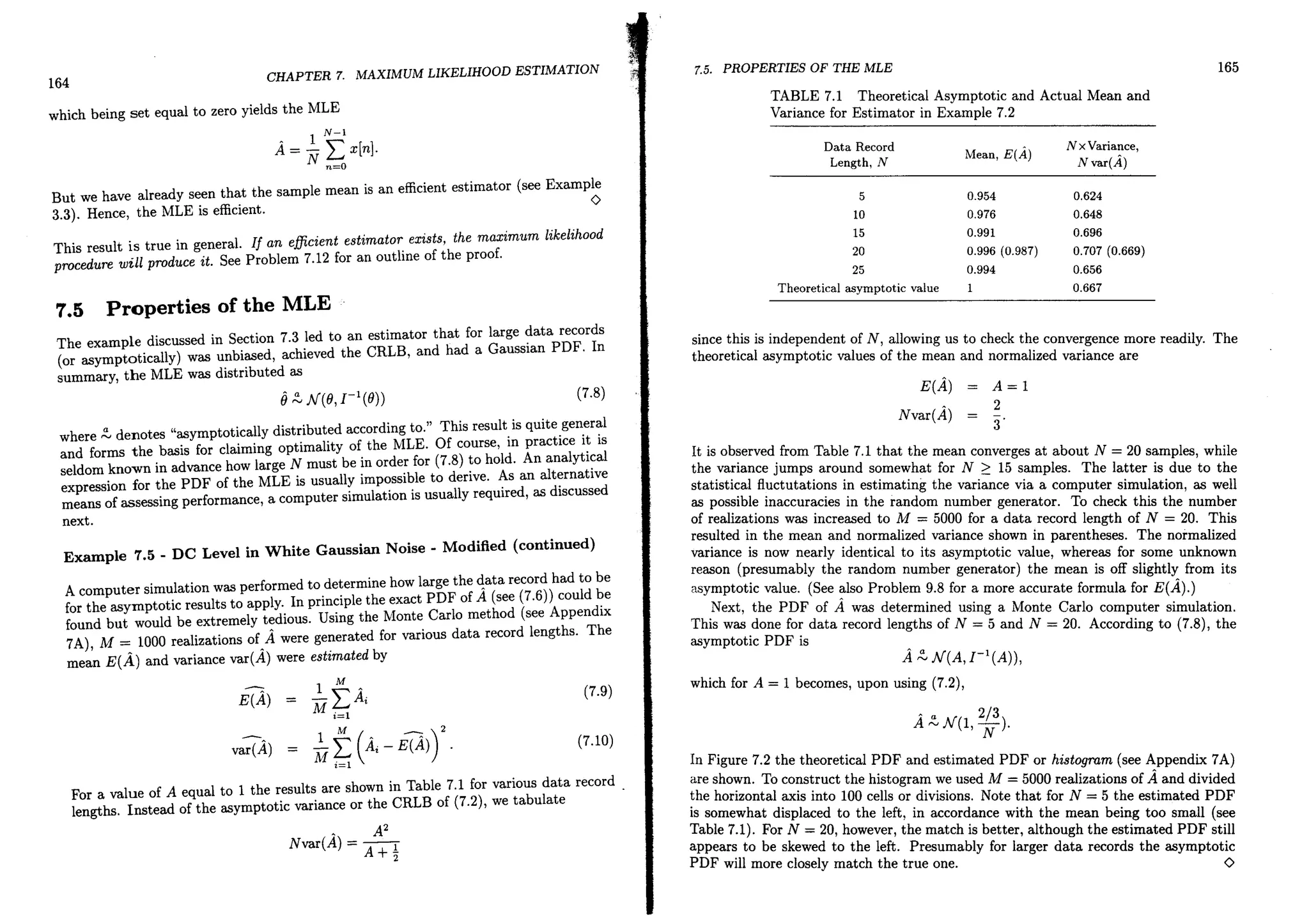
![166 CHAPTER 7. MAXIMUM LIKELIHOOD ESTIMATION
1.25 -T
0.94-+
0.624
,
I
0.31-+
O.OO-i'---------j~=------r___----"'-'--p____----_, A
3.00
-1.00
2.50'1
,
I
I
1.88-+
I
i
1.25-+
062~I
0.00 1.00 2.00
(a) N = 5
O.OO4------~~----~----~~-----~
0.00 0.50 1.00 1.50 2.00
(b) N=20
Figure 7.2 Theoretical PDF and histogram
In describing the performance of estimators whose PDFs cannot be determined analyt-
ically, we must frequently resort to computer simulations, as in the previous example.
In practice, the computer has become the dominant tool for analyzing the performance
of nonlinear estimators. For this reason it is important to be able to carry out such
a simulation. In Appendix 7A a description of the computer methods used in the
previous example is given. Of course, the subject of Monte Carlo computer methods
for statistical evaluation warrants a more complete discussion. The interested reader
should consult the following references: [Bendat and Piersol 1971, Schwartz and Shaw
7.5. PROPERTIES OF THE MLE 167
1975]. Some practice in performing these simulations is provided by Problems 7.13 and
7.14. We now summarize the asymptotic properties of the MLE in a theorem.
Theorem 7.1 (Asymptotic Properties of the MLE) If the PDF p(x; 8) of the
data x satisfies some "re ularit " conditions, then the MLE of the unknown parameter
B is asymptotzcaUy distributed (for large ata recon s according to
(7.11)
where I(B) is the Fisher information evaluated at the true value of the unknown param-
eter.
The regularity conditions require the existence of the derivatives of the log-likelihood
function, as well as the Fisher information being nonzero, as described more fully in
Appendix 7B. An outline of the proof for lID observations is also given there.
From the asymptotic distribution, the MLE is seen to be asymptotically unbiased
and asymptotically attains the CRLB. It is therefore asymptotically efficient, and hence
asymptotically optimaL Of course, in practice the key question is always How large
does N have to be for the asymptotic properties to apply? Fortunately, for many cases
or interest the data record lengths are not exceSSive, as illustrated by Example 7.5.
Another example follows.
Example 7.6 - MLE of the Sinusoidal Phase
We now reconsider the problem in Example 3.4 in which we wish to estimate the phase
I/> of a sinusoid embedded in noise or
x[n] = A cos(271'fon +¢) + w[n] n = O,l, ... ,N - 1
where w[n] is WGN with variance (J'2 and the amplitude A and frequency fo are assumed
to be known. We saw in Chapter 5 that no single sufficient statistic exists for this
problem. The sufficient statistics were
N-I
TI(x) = L x[n]cos(27l'fon)
n=O
N-I
T2 (x) = L x[n] sin(27l'Jon). (7.12)
n=O
The MLE is found by maximizing p(x; 1/» or
p(x; 1/» = N exp --2 L (x[n]- Acos(27l'fon +¢))2
1 [1 N-I ]
(27l'(J'2) T 2(J' n=O
or, equivalently, by minimizing
N-I
J(I/» = L (x[n]- Acos(27l'fon + 1/»)2. (7.13)
n=O](https://image.slidesharecdn.com/fundamentalsofstatisticalsignalprocessing-estimationtheory-kay-230513154707-1f7652e0/75/Fundamentals-Of-Statistical-Signal-Processing-Estimation-Theory-Kay-pdf-89-2048.jpg)
![168 CHAPTER 7. MAXIMUM LIKELIHOOD ESTIMATION
Differentiating with respect to <I> produces
8J(<I» N-I
----a¢ = 2 L (x[n]- Acos(21l'fon + <1») Asin(21l'fon + <1»
n=O
and setting it equal to zero yields
N-I N-I
L x[n]sin(21l'fon+¢) = A L sin(21l'fon+~)cos(21l'fon+¢). (7.14)
n=O n=O
But the right-hand side may be approximated since (see Problem 3.7)
1 N-I , , 1 N-I ,
N L sin(21l'fon + <1» cos(21l'fon + <1» = 2N L sin(41l'fon + 2<1» ~ 0
n=O n=O
(7.15)
for fo not near 0 or 1/2. Thus, the left-hand side of (7.14) when divided by N and set
equal to zero will produce an approximate MLE, which satisfies
N-I
L x[n] sin(21l'fon +¢) = o. (7.16)
n=O
Upon expanding this we have
N-I N-I
L x[n] sin 21l'fon cos¢ = - L x[n] cos 21l'fonsin¢
n=O n=O
or finally the MLE of phase is given approximately as
N-I
L x[n] sin 21l'fon
'" n=O
<I> = - arctan 7'
N
c:.:_.::.
I
- - - - - (7.17)
Lx[n] cos 21l'fon
n=O
It is interesting to note that the MLE is a function of the sufficient statistics. In hind-
sight, this should not be surprising if we keep in mind the Neyman-Fisher factorization
theorem. In this example there are two sufficient statistics, effecting a factorization as
p(X;<I» = g(TI (x),T2 (x),<I»h(x).
Clearly, maximizing p(x;<I» is equivalent to maximizing 9 (h(x) can always be chosen
so that h(x) > 0), and thus ¢ must be a function of TI(X) and T2(X),
According to Theorem 7.1, the asymptotic PDF of the phase estimator is
(7.18)
7.5. PROPERTIES OF THE MLE
TABLE 7.2 Theoretical Asymptotic and Actual Mean and
Variance for Estimator in Example 7.6
Data Record
Mean, E(d»
Length, N
20 0.732
40 0.746
60 0.774
80 0.789
Theoretical asymptotic value ¢ = 0.785
From Example 3.4
so that the asymptotic variance is
1(<1» = NA2
2a2
, 1 1
var(<1» = ---:42 = -
N 2,,2 N"1
NxVariance,
Nvar(¢)
0.0978
0.108
0.110
0.0990
liT! = 0.1
169
(7.19)
where "1 = (A2
/2)/a2
is the SNR. To determine the data record length for the asymp-
totic mean and variance to apply we performed a computer simulation using A = 1, fo =
0.08, <I> = 1l'/4, and a 2
= 0.05. The results are listed in Table 7.2. It is seen that the
asymptotic mean and normalized variance are attained for N = 80. For shorter data
records the estimator is considerably biased. Part of the bias is due to the assumption
made in (7.15). The MLE given by (7.17) is actually valid only for large N. To find the
exact MLE we would have to minimize J as given by (7.13) by evaluating it for all <1>.
This could be done by using a grid search to find the minimum. Also, observe from the
table that the variance for N = 20 is below the CRLB. This is possible due to the bias
of the estimator, thereby invalidating the CRLB which assumes an unbiased estimator.
Next we fixed the data record length at N = 80 and varied the SNR. Plots of the
mean and variance versus the SNR, as well as the asymptotic values, are shown in
Figures 7.3 and 7.4. As shown in Figure 7.3, the estimator attains the asymptotic
mean above about -10 dB. In Figure 7.4 we have plotted 10 10glO var(¢). This has the
desirable effect of causing the CRLB to be a straight line when plotted versus the SNR
in dB. In particular, from (7.19) the asymptotic variance or CRLB is
10 10giO var(¢)
1
1010gi0 N"1
-10 10glO N - 10 10giO "1.
Examining the results, we see a peculiar trend. For low SNRs the variance is higher
than the CRLB. Only at higher SNRs is the CRLB attained. Hence, the required
data record length for the asymptotic results to apply also depends on the SNR. To](https://image.slidesharecdn.com/fundamentalsofstatisticalsignalprocessing-estimationtheory-kay-230513154707-1f7652e0/75/Fundamentals-Of-Statistical-Signal-Processing-Estimation-Theory-Kay-pdf-90-2048.jpg)
![170 CHAPTER 7. MAXIMUM LIKELIHOOD ESTIMATION
• I •••• ~ ••••.••••••s
0.651--------rI-------4I--------rl-------.I--------r
l ------~I
-20 -15 -10 -5 0 5 10
SNR (dB)
Figure 7.3 Actual vs. asymptotic mean for phase estimator
0,
-5--+......
i-LO~ ••• j
..............
> -15-+
; -20J
o ,
Asymptotic variance
"" - 251
-30 I I I I I
-15 -10 -5 0 5
SNR (dB)
Figure 7.4 Actual vs. asymptotic variance for phase estimator
understand why this occurs we plot typical realizations of the log-likelihood function
for different SNRs. As seen in Figure 7.5 for a high SNR, the maximum is relatively
stable from realization to realization, and hence the MLE exhibits a low variance. For
lower SNRs, however, the effect of the increased noise is to cause other peaks to occur.
Occasionally these peaks are larger than the peak near the true value, causing a large
estimation error and ultimately a larger variance. These large error estimates are said
to be outliers and cause the threshold effect seen in Figures 7.3 and 7.4. Nonlinear
estimators nearly always exhibit this effect. <>
7.5. PROPERTIES OF THE MLE
171
I:)
:::
.S -20
..-
u
-30
:::
.z -40
"0
0
"i
0
:-S -{i0
-.;
3 -70
~
0 -80
...l
-90
-100
-3 -2 -1 0 2 3
Phase, ¢
(a) High SNR (10 dB)
0
-1O~
:::
-20~
.~
~ -30
..§
-40
"5 = -
0 -50
:9 -{i0
~
70
-70
0 -80
...l
-90 .
. .
-100 <PI :¢2 :¢3
-3 -2 -1 0 2 3
True <P
Phase, ¢
(b) Low SNR (-15 dB)
Figure 7.5 Typical realizations of log-likelihood function for phase
In su.mma~y, th~ asymptotic PDF of the MLE is valid for large enough data records.
For slgna~ III .nOlse problems the CRLB may be attained even for short data records if
the SNR IS high enough. To see why this is so the phase estimator can be written from
(7.17) as
N-I
L [Acos(21!'fon + ¢J) + w[n]] sin 21!'fon
~ - arctan r;;~=~~'---------------------
L [A cos(21!'fon +¢J) + w[n]] cos 211'fon
n=O](https://image.slidesharecdn.com/fundamentalsofstatisticalsignalprocessing-estimationtheory-kay-230513154707-1f7652e0/75/Fundamentals-Of-Statistical-Signal-Processing-Estimation-Theory-Kay-pdf-91-2048.jpg)
![172 CHAPTER 7. MAXIMUM LIKELIHOOD ESTIMATION
p(w[n)) p(x[nJ;A)
w[nJ
A
x[nJ
(a) (b)
Figure 7.6 Non-Gaussian PDF for Example 7.7
N-l
- N2A sin ¢> + L w[n] sin 211"fon
~ _ arctan ____---,-:-:n==o:.0_____
N-l
N2A cos ¢> + L w[n] cos 211"fon
n=O
where we have used the same type of approximation as in (7.15) and some standard
trigonometric identities. Simplifying, we have
N-l
sin¢>- ;ALw[n]sin211"fon
J~ arctan n=O
N-l (7.20)
cos ¢> + ;A L w[n] cos 211"fon
n=O
If the data record is large and/or the sinusoidal power is large, the noise terms will be
small. It is this condition, that the estimation error is small, that allows the MLE to
attain its asymptotic distribution. See also Problem 7.15 for a further discussion of this
point.
In some cases the asymptotic distribution does not hold, no matter how large the
data record and/or the SNR becomes. This tends to occur when the estimation error
cannot be reduced due to a lack of averaging in the estimator. An example follows.
Example 7.7 - DC Level in Nonindependent Non-Gaussian Noise
Consider the observations
x[n] = A + w[n] n = 0, 1, ... ,JV - 1
where each sample of w[n] has the PDF p(w[n]) as shown in Figure 7.6a. The PDF is
symmetric about w[nJ =0 and has a maximum at w[n] = o. Furthermore, we assume
all the noise samples are equal or w[OJ = w[IJ = ... = w[JV - IJ. In estimating A we
need to consider only a single observation since all observations are identical. Utilizing
7.6. MLE FOR TRANSFORMED PARAMETERS 173
only x[O], we first note that the PDF of x[O] is a shifted version of p(w[n]), where the
shift is A as shown in Figure 7.6b. This is because Px[Oj(x[OJ; A) = PW[Oj(x[OJ - A). The
MLE of A is the value that maximizes Pw[Oj(x[O]- A), which because the PDF of w[OJ
has a maximum at w[OJ = 0 becomes
A=x[OJ.
This estimator has the mean
E(A) = E(x[O]) = A
since the noise PDF is symmetric about w[OJ = o. The variance of Ais the same as the
variance of x[O] or of w[O]. Hence,
var(A) = I:U
2
PW[Oj(U) du
while the CRLB, is from Problem 3.2,
and the two are not in general equal (see Problem 7.16). In this example, then, the
estimation error does not decrease as the data record length increases but remains the
same. Furthermore, the PDF of A= x[OJ as shown in Figure 7.6b is a shifted version
of p(w[n]), clearly not Gaussian. Finally, Ais not even consistent as JV -+ 00. 0
7.6 MLE for Transformed Parameters
In many instances we wish to estimate a function of () the arameter charac erizin
the P . or example, we may no e mteres e in the value of a DC level A in WGN
but only in the power A2. In such a situation the MLE of A2 is easily found from the
MLE of A. Some examples illustrate how this is done.
Example 7.8 - 'fransformed DC Level in WGN
Consider the data
x[n] = A +w[n] n = 0, 1, ... ,JV - 1
where w[n] is WGN with variance (]"2. We wish to find the MLE of Q = exp(A). The
PDF is given as
1 [1 N-l ]
p(x; A) = N exp --2
2 L (x[nJ - A?
(211"(]"2) "2 (]" n=O
-oo<A<oo (7.21)](https://image.slidesharecdn.com/fundamentalsofstatisticalsignalprocessing-estimationtheory-kay-230513154707-1f7652e0/75/Fundamentals-Of-Statistical-Signal-Processing-Estimation-Theory-Kay-pdf-92-2048.jpg)
![174 CHAPTER 7. MAXIMUM LIKELIHOOD ESTIMATION
and is parameterized by the parameter e = A. However, since a is a one-to-one
transformation of A, we can equivalently parameterize the PDF as
PT(x;a) = 1 N exp [-- I:(X[nJ-Ina)2]
(211'0.2)2 20' n=O
a>O (7.22)
where the subscript T indicates that the PDF is parameterized according to the trans-
formed parameter. Clearly, PT(X; a) is the PDF of the data set
x[nJ=lna+w[nJ n=O,l, ... ,N-l
and (7.21) and (7.22) are entirely equivalent. The MLE of a is found by maximizing
(7.22) over a. Setting the derivative of PT(x;a) with respect to a equal to zero yields
N-I 1
L (x[nJ-Ina)-;:- = 0
n=O a
or
a =exp(x).
But x is just the MLE of A, so that
a = exp(A) = exp(B).
The MLE of the transformed parameter is found by substituting the MLE of the original
parameter mto the transformatIOn. ThIS property of the MLE is termed the invanance·'
property. '
Example 1.9 - Transformed DC Level in WGN (Another Example)
Now consider the transformation a = A2 for the data set in the previous example. If
we try to repeat the steps, we soon encounter a problem. Attempting to parameterize
p(x; A) with respect to a, we find that
A=±vIa
since the transformation is not one-to-one. If we choose A = ,;a, then some of the
possible PDFs of (7.21) will be missing. We actually require two sets of PDFs
PT, (x; a) = 1 N exp [-- ~I(x[nJ- vIa)2] a ~ 0
(211'0'2)2 20' n=O
PT. (x; a) = 1 N exp [-212 ~x[nJ + val] a> 0 (7.23)
(211'0'2) 2 0' n=O
to characterize all possible PDFs. It is possible to find the MLE of a as the value of a
that yields the maximum of PT,(x; a) and PT. (x; a) or
a = arg max {PT, (x; a), PT. (x; a)}. (7.24)
"
Alternatively, we can find the maximum in two steps as
7.6. MLE FOR TRANSFORMED PARAMETERS
175
p(x;A)
Ao
A
PT,(x;a)
PT2 (x;a)
...........
..... ......
.'
...
a
ftr(x; a) = max {PTl (x; a), PT. (x; a)}
a
Figure 7.7 Construction of modified likelihood function
1. Fo; a given value of a, say ao, determine whether PT (x; a) or Pr (x' a) is larger If
lOr example, 1 2 , • ,
PT,(x; ao) > PT2 (x; ao),
~he(n de)no(~ the value of PT, (x; ao) as PT(X; ao). Repeat for all a > 0 to form
PT x; a. ote that PT(X; a = 0) = p(x; A = 0).)
2. The MLE is given as the a that maximizes PT(X; a) over a ~ o.
'::5p,roced.ure. is illustrated in Fi?ure 7.7. The function fiT (x; a) can be thought of as
b tdifi~d lzk:Mood functzon, havmg been derived from the original likelihood function
y rans ormmg the value of A that yields the maximum value for a given a In this
example, for each a the possible values of A are ±,;a. Now, from (7.24) the MLE Q is
arg max {p(x; va),p(x; -va)}
"2:0](https://image.slidesharecdn.com/fundamentalsofstatisticalsignalprocessing-estimationtheory-kay-230513154707-1f7652e0/75/Fundamentals-Of-Statistical-Signal-Processing-Estimation-Theory-Kay-pdf-93-2048.jpg)
![176
CHAPTER 7. MAXIMUM LIKELIHOOD ESTIMATION
[
arg max {p(x; va),p(x; -va) })2
va~o
[
arg max p(x; A))2
-oo<A<oo
iF
x2
so that again the invariance property holds. The understan~in~ is that 0: ~axi~izes
the modified likelihood function pr(x; 0:) since the standard hkehhood function with ~
as a parameter cannot be defined.
We summarize the preceding discussion in the following theorem.
Theorem 7.2 (Invariance Property o.f the ML~) The MLE of the pammeter 0: =
gj!!), where the PDF p(x; 0) is pammete1"lzed by 0, tS gwen by
0: = g(O)
j)r(X;O:) = max p(x;O).
{8:a=g(8)}
We complete our discussion by giving another example.
Example 7.10 - Power of WGN in dB
N I f WGN with variance a2 whose power in dB is to be estimated.
We observe samp es 0 . ' . ' I t fi d the
To do so we first find the MLE of a2
. Then, we use the mvanance prmcJP eon
power P in dB, which is defined as
P = 10 10gJO a
2
•
The PDF is given by
p(x;a2 ) = 1 J:i.. exP[-2121:x2[nJ).
(27ra2) 2 a n=O
Differentiating the log-likelihood function produces
8Inp(x;a
2
) = ~ [_N In27r _ N Ina2 - 2121: x2
[nJ)
8a2 8a2 2 2 a n=O
N 1 N-J
= --+-L x2 [nJ
2a2
2a4
n=O
7.7. NUMERICAL DETERMINATION OF THE MLE 177
p(x;lf)
If
a O=MLE b Figure 7.8 Grid search for MLE
and upon setting it equal to zero yields the MLE
The MLE of the power in dB readily follows as
P 1010glO;2
1 N-I
1OioglO N L x
2
[nJ.
n=O
7.7 Numerical Determination of the MLE
o
A distinct advantage of the MLE is that we can always find it for a given data set
numerically. This is because the MLE is determined as the maximum of a known
function, namely, the likelihood function. If, for example, the allowable values of () lie
in the interval [a, b], then we need only maximize p(x; 0) over that interval. The "safest"
way to do this is to perform a grid search over the [a, bJ interval as shown in Figure 7.8.
As long as the spacing between 0 values is small enough, we are guaranteed to find the
MLE for the given set of data. Of course, for a new set of data we will have to repeat
the search since the likelihood function will undoubtedly change. If, however, the range
of 0 is not confined to a finite interval, as in estimating the variance of a noise process
for which a 2
> 0, then a grid search may not be computationally feasible. In such a
case, we are forced to resort to iterative maximization procedures. Some typical ones are
the Newton-Raphson method, the scoring approach, and the expectation-maximization
algorithm. In general, these methods will produce the MLE if the initial guess is close
t.o the true maximum. If not, convergence may not be attained, or only convergence to a
iocal maximum. The difficulty with the use of these iterative methods is that in general
we do not know beforehand if they will converge and, even if convergence is attained,
whether the value produced is the MLE. An important distinction of our estimation
problem which sets it apart from other maximization problems is that the function to
be maximized is not known a priori. The likelihood function changes for each data set,](https://image.slidesharecdn.com/fundamentalsofstatisticalsignalprocessing-estimationtheory-kay-230513154707-1f7652e0/75/Fundamentals-Of-Statistical-Signal-Processing-Estimation-Theory-Kay-pdf-94-2048.jpg)
![178 CHAPTER 7. MAXIMUM LIKELIHOOD ESTIMATION
requiring the maximization of a random function. Nevertheless, these methods can at
times produce good results. We now describe some of the more common ones. The
interested reader is referred to [Bard 1974] for a more complete description of methods
for nonlinear optimization as applied to estimation problems.
As a means of comparison, we will apply the methods to the following example.
Example 7.11 - Exponential in WGN
Consider the data
x[n] = rn +w[n] n = 0, 1, ... , N - 1
where w[n] is WGN with variance (J'2. The parameter r, the exponential factor, is to
be estimated. Allowable values are r > o. The MLE of r is the value that maximizes
the likelihood function
or, equivalently, the value that minimizes
N-l
J(r) = L (x[n]- rn)2 .
n=O
Differentiating J(r) and setting it equal to zero produces
N-l
L (x[n]- rn) nrn- 1
= o. (7.25)
n=O
This is a nonlinear equation in r and cannot be solved directly. We will now consider
the iterative methods of Newton-Raphson and scoring. 0
The iterative methods attempt to maximize the log-likelihood function by finding a
zero of the derivative function. To do so the derivative is taken and set equal to zero,
yielding
alnp(x; 9) = 0
a9 . (7.26)
Then, the methods attempt to solve this equation iteratively. Let
(
9) = alnp(x; 9)
9 a9
and assume that we have an initial guess for the solution to (7.26). Call this guess 90 ,
Then, if g(9) is approximately linear near 90 , we can approximate it by
dg(9) ·1
g(9) ~ g(90 ) + dJJ 8=80 (9 - 90 ) (7.27)
.. - - ~ - - - ~ - - ~ ~ - - - - -~ ----- - - ~ -
7.7. NUMERICAL DETERMINATION OF THE MLE 179
(J Figure 1.9 Newton-Raphson
method for finding zero of function
as shown in Figure 7.9. Next, we use (7.27) to solve for the zero 91, so that upon setting
g(91 ) equal to zero and solving for 91 we have
Again w~ linearize 9 but use the new guess, 91 , as our point of linearization and repeat
the prevlOUS procedure to find the new zero. As shown in Figure 7.9, the sequence of
guesses will converge to the true zero of g(9). In general, the Newton-Raphson iteration
finds the new guess, 9k +1 , based on the previous one, 9k , using
9k
+1
= 9k
- dg(9) I
d9 8=8.
(7.28)
Note that at convergence 9k +1 = 9k , and from (7.28) g(9k ) = 0, as desired. Since g(9)
is the derivative of the log-likelihood function, we find the MLE as
9 =9 _ [a2Inp(X;9)]-lalnp(X;9)1
k+1 k a92 a9
8=8.
(7.29)
Several points need to be raised concerning the Newton-Raphson iterative procedure.
1. The iteration may not converge. This will be particularly evident when the second
derivative of the. log-likelihood function is small. In this case it is seen from (7.29)
that the correctlOn term may fluctuate wildly from iteration to iteration.
2. Even if the iteration converges, the point found may not be the global maximum but
possibly only a local maximum or even a local minimum. Hence, to avoid these
possibilities it is best to use several starting points and at convergence choose the
one ~hat yields .the n:axi~um. Generally, if the initial point is close to the global
maxImUm, the IteratlOn Will converge to it. The importance of a good initial guess
cannot be overemphasized. An illustration is given in Problem 7.18.](https://image.slidesharecdn.com/fundamentalsofstatisticalsignalprocessing-estimationtheory-kay-230513154707-1f7652e0/75/Fundamentals-Of-Statistical-Signal-Processing-Estimation-Theory-Kay-pdf-95-2048.jpg)
![180 CHAPTER 7. MAXIMUM LIKELIHOOD ESTIMATION
Applying the Newton-Raphson iteration to the problem in Example 7.11, we have
olnp(x; r)
or
02Inp(x; r)
or2
1 N-l
- '" (x[nJ - rn)nrn- 1
a2 L...J
n=O
1 [N-l N-l ]
a2 ?;n(n - 1)x[nJr
n
- 2- ?;n(2n - 1)r2n- 2
1 N-l
2' L nrn- 2
[(n -l)x[nJ - (2n - l)rnJ
a n=O
and thus the Newton-Raphson iteration becomes
N-l
L (x[nJ - r;:)nr;:-l
n=O
rk+l = rk - .,-N,.---l----.:..::=----------
L nr;:-2 [(n - l)x[nJ - (2n - l)r;:J
n=O
(7.30)
(7.31)
A second common iterative procedure is the method of scoring. It recognizes that
where /(9) is the Fisher information. Indeed, for lID samples we have
02
In p(x; 9)
092
'~ 02Inp(x[nJ; 9)
L...J 092
n=O
N ~ tl02Inp(x[nJ; 9)
N n=O 092
:::::J NE [0
2
Inp(x[nJ; 9)]
092
-Ni(9)
= -1(9)
(7.32)
by the law of large numbers. Presumably, replacing the second derivative by its expected
value will increase the stability of the iteration. The method then becomes
D = D I-1 (D)0In p(x;9) I
Uk+! uk + U 09 .
8=8.
(7.33)
This approach is termed the method of scoring. It too suffers from the same convergence
problems as the Newton-Raphson iteration. As applied to the problem in Example 7.11,
7.7. NUMERICAL DETERMINATION OF THE MLE
TABLE 7.3 Sequence of Iterates
for Newton-Raphson Method
Iteration
2
3
4
5
6
7
8
9
10
29
Initial Guess, ro
0.8 0.2 1.2
0.723 0.799 1.187
0.638 0.722 1.174
0.561 0.637 1.161
0.510 0.560 1.148
0.494 0.510 1.136
0.493 0.494 1.123
0.493 1.111
1.098
1.086
1.074
0.493
it produces upon using (7.30)
so that
N-l
L (x[nJ - r;:)nr;:-l
n=O
rk+! = rk + -==~N:-:---l"'-----
Ln2
rzn
-
2
n=O
181
(7.34)
As an example of the iterative approach, we implement the Newton-Raphson method
for Example 7.11 using a computer simulation. Using N = 50, r = 0.5, and a2
=0.01,
we generated a realization of the process. For a particular outcome -J(r) is plotted
in Figure 7.10 for 0 < r < 1. The peak of the function, which is the MLE, occurs
at r = 0.493. It is seen that the function is fairly broad for r < 0.5 but rather sharp
for larger values of r. In fact, for r > 1 it was difficult to plot due to the exponential
signal r n
, which causes the function to become very large and negative. We applied the
Newton-Raphson method as given by (7.31) using several initial guesses. The resulting
iterates are listed in Table 7.3. For ro = 0.8 or ro = 0.2 the iteration quickly converged
to the true maximum. However, for ro = 1.2 the convergence was much slower, although
the true maximum was attained after 29 iterations. If the initial guess was less than
about 0.18 or greater than about 1.2, the succeeding iterates exceeded 1 and kept](https://image.slidesharecdn.com/fundamentalsofstatisticalsignalprocessing-estimationtheory-kay-230513154707-1f7652e0/75/Fundamentals-Of-Statistical-Signal-Processing-Estimation-Theory-Kay-pdf-96-2048.jpg)
![182 CHAPTER 7. MAXIMUM LIKELIHOOD ESTIMATION
N-l
- L(x[nl- rn)2
n=O
0.00
-{).75
-1.50
-2.25
r == 0.493 ~ /True r == 0.5
-3.00+-----r-------=~r=_----___r--~--___j
0.00 0.25 0.50 0.75 1.00
r
Figure 7.10 Function to be maximized for MLE
increasing, causing a computer overflow condition in the algorithm. In this case the
Newton-Raphson method fails to converge. As expected, the method works well when
the initial guess is close to the true MLE but may produce poor results otherwise.
A third method that has recently been proposed is the expectation-maximization
algorithm. Unlike the first two methods, it requires some ingenuity on the part of
the designer. Its advantage, however, is its guaranteed convergence to at ~east a.local
maximum under some mild conditions. Convergence to the global maxImum IS, as
with all iterative schemes, not assured. The expectation-maximization algorithm, not
being a "turn-the-crank" procedure, does not lend itself to all estimation problems. A
particular class of problems for which it is useful involves a vector parameter, and so
we defer our discussion until the next section.
7.8 Extension to a Vector Parameter
The MLE for a vector parameter 6 is defined to be the value that maximizes the
likelihood function p(x; 6) over the allowable domain for 6. Assuming a differentiable
likelihood function, the MLE is found from
8Inp(xj6) =0.
86
(7.35)
If multiple solutions exist, then the one that maximizes the likelihood function is the
MLE. We now find the MLE for the problem in Example 3.6.
7.B. EXTENSION TO A VECTOR PARAMETER
183
Example 1.12 - DC Level in WGN
Consider the data
x[nJ = A +w[nJ n = 0, 1, ... ,N - 1
where w[nJ is WGN with variance 0'2 and the vector parameter 6 = [A 0'2]T is to be
estimated. Then, from Example 3.6
8Inp(x;6)
8A
8Inp(x;6)
80'2
1 N-l
2 L(x[nJ -A)
a n=O
N 1 N-l
--2
2 + -2
4 L (x[nJ - A)2.
a a n=O
Solving for A from the first equation, we have the MLE
A=x.
Solving for 0'2 in the second equation and using A= x produces
A 1 N-l
0'2 = N L(x[nJ - x?
n=O
The MLE is
{J = [ 1 N-l X j.
N ~ (x[nJ - X)2
<>
For a vector parameter the asYIJ?ptotic properties of the MLE are summarized in the
following theorem.
';:'heorem 1.3 (Asymptotic Properties of the MLE (Vector Parameter» If the
PDF p(Xj 6) of the data x satisfies some "regularity" conditions, then the MLE of the
unknown parameter 6 is asymptotically distributed according to
(7.36)
where 1(6) is the Fisher information matrix evaluated at the true value of the unknown
parameter.
The regularity conditions are similar to those discussed in Appendix 7B for the scalar
parameter case. As an illustration, consider the previous example. It can be shown
~hat [Hoel, Port, and Stone 1971J
(7.37)](https://image.slidesharecdn.com/fundamentalsofstatisticalsignalprocessing-estimationtheory-kay-230513154707-1f7652e0/75/Fundamentals-Of-Statistical-Signal-Processing-Estimation-Theory-Kay-pdf-97-2048.jpg)
![--r-~"""'-""'~-----"-- ~-~---~----~ ...
184 CHAPTER 7. MAXIMUM LIKELIHOOD ESTIMATION
and that the two statistics are independent. For large N it is well known from the
central limit theorem that
x~ :;. N(N, 2N)
so that
T:;' N(N - 1, 2(N - 1))
or
. 1 N-I _ 2 a ((N -1)a2. 2(N -1)a4
)
a2 = N 2)x[n]-x) ",N N ' N2 .
n=O
(7.38)
The asymptotic PDF of 8is jointly Gaussian since the statistics are individually Gaus-
sian and independent. Furthermore, from (7.37) and (7.38) for large N
E(8)
[ (N ;1)a' 1-+ [~ ] = 9
[~
0
1
[a' 0
1
--+ N
2a4 = rl(9)
2(N - l)a4
0
N2 N
C(9) =
where the inverse of the Fisher information matrix has previously been given in Example
3.6. Hence, the asymptotic distribution is described by (7.36).
In some instances, the asymptotic PDF of the MLE is not given by (7.36). These
situations generally occur when the number of parameters to be estimated is too large
relative to the number of data samples available. As in Example 7.7, this situation
restricts the averaging in the estimator.
Example 1.13 - Signal in Non-Gaussian Noise
Consider the data
x[n] = s[n] +w[n] n = 0, 1, .. . ,N - 1
where w[n] is zero mean lID noise with the Laplacian PDF
p(w[n]) = ~ exp [-~Iw[nll] .
The signal samples {s[O], s[I], . .. ,s[N - I]} are to be estimated. The PDF of the data
is
N-I 1 [1 ]
p(xj9) = II 4exp -2Ix[n]-s[n]1 .
n=O
(7.39)
The MLE of 9 = [s[O] s[I] ... s[N - 1]jT is easily seen to be
s[n] = x[n] n = 0,1, ... ,N - 1
.... ---------------_ ......... .
7.S. EXTENSION TO A VECTOR PARAMETER 185
or, equivalently,
8= x.
It is clear that the MLE is not Gaussian even as N -+ 00. The PDF of 8 is given by
(7.39) with x replaced by 8. The difficulty is that no averaging is possible since we
have chosen to estimate as many parameters as data points. Therefore, the central limit
theorem, which accounts for the asymptotic Gaussian PDF of the MLE (see Appendix
7B), does not apply. <)
As in the scalar case, the invariance property holds, as summarized by the following
theorem.
Theorem 1.4 (Invariance Property of MLE (Vector Parameter» The MLE of
the parameter a = g(9), where g is an r-dimensional function of the p x 1 parameter
9, and the PDF p(Xj 9) is parameterized by 9, is given by
it = g(8)
for 8, the MLE of 9. If g is not an invertible function, then it maximizes the modified
likelihood function PT(Xj a), defined as
PT(Xj a) = max p(x; 9).
{B:a=g(B)}
An example of the use of this theorem can be found in Problem 7.2l.
In Chapter 3 we discussed the computation of the CRLB for the general Gaussian
case in which the observed data vector had the PDF
X'" N(Jl.(9), C(9)).
In Appendix 3C (see (3C.5)) it was shown that the partial derivatives of the log-
likelihood function were
8Inp(x; 9)
8(h
for k = 1,2, ... ,p. By setting (7.40) equal to zero we can obtain necessary conditions
for the MLE and on occasion, if solvable, the exact MLE. A somewhat more convenient
form uses (3C.2) in Appendix 3C to replace 8C-I(9)/8(h in (7.40). An important
example of the latter is the linear model described in detail in Chapter 4. Recall that
the general linear data model is
x = H9+w (7.41)
where H is a known N x p matrix and w is a noise vector of dimension N x 1 with PDF
N(O, C). Under these conditions the PDF is
p(x; 9) = IV 1 1 exp [--2
1
(x - H9)TC- I
(x - H9)]
(27r)T det2(C)](https://image.slidesharecdn.com/fundamentalsofstatisticalsignalprocessing-estimationtheory-kay-230513154707-1f7652e0/75/Fundamentals-Of-Statistical-Signal-Processing-Estimation-Theory-Kay-pdf-98-2048.jpg)
!['IAIAAIA.III •••••• · · · · · · · - -
186
CHAPTER 7. MAXIMUM LIKELIHOOD ESTIMATION
so that the MLE of 6 is found by minimizing
J(6) = (x - H6fe-l (x - H6). (7.42)
Since this is a quadratic function of the elements of 6 and e-l
.is a positive defi~ite
matrix, differentiation will produce the global minimum. Now, usmg (7.40) and notmg
that
,.,,(6) = H6
and that the covariance matrix does not depend on 6, we have
8lnp(x;6) = 8(H6)T e-l(x-H6).
8fh 80k
Combining the partial derivatives to form the gradient, we have
8lnp(x;6) = 8(H6f e-l(x-H6)
86 86
so that upon setting the gradient equal to zero we have
HTe-l(x - H8) =o.
Solving for {j produces the MLE
8 = (HTe-1H)-IHTe-lx. (7.43)
But this estimator was shown in Chapter 4 to be the MVU estimator as well as an
efficient estimator. As such, 8 is unbiased and has a covariance of
eli = (HTe-1H)-I. (7.44)
F· 11 th PDF of the MLE is Gaussian (being a linear function of x), so that the
~;~~oticeproperties of Theorem 7.3 are attained even for finite data records. ~or the
linear model it can be said that the MLE is optimal. These results are summarized by
the following theorem.
Theorem 7.5 (Optimality of the MLE for the Linear Model) If the observed
data x are described by the general linear model
x = H6 + w (7.45)
where H is a known N x p matrix with N > p and of rank p, 6 is a p x 1 parameter
vector to be estimated, and w is a noise vector with PDF N(O, C), then the MLE of 6
is
8 = (HTe-1H)-IHTe-lx. (7.46)
8 is also an efficient estimator in that it attains the CRLB and hence is the MVU
estimator. The PDF of 8 is
(7.47)
,.------------------_ ....... .
7.B. EXTENSION TO A VECTOR PARAMETER 187
Many examples are given in Chapter 4. The preceding result can be generalized to
assert that if an efficient estimator exists, it is given by the MLE (see Problem 7.12).
In finding the MLE it is quite common to have to resort to numerical techniques of
maximization. The Newton-Raphson and scoring methods were described in Section
7.7. They are easily extended to the vector parameter case. The Newton-Raphson
iteration becomes
6 =fJ _ [8
2
Inp(X;fJ)]-1 8Inp(x;fJ)I
k+l k 8fJ8fJT 8fJ
9=9.
(7.48)
where
[
82
In p(X;fJ)] 82Inp(x;fJ) i=I,2, ... ,p
8fJ86T ij 88i 88j j = 1,2, ... ,p
is the Hessian of the log-likelihood function and alnb~x;9) is the p x 1 gradient vector.
In implementing (7.48) inversion of the Hessian is not required. Rewriting (7.48) as
8
2
Inp(X;fJ)/ fJ = 8
2
Inp(X;fJ)/ fJ _ 8Inp(x;fJ)/ (7.49)
8fJ8fJT 9=9. k+l 8fJ86T 9=9. k 8fJ 9=9.
we see that the new iterate, fJk+l, can be found from the previous iterate, 6k , by solving
a set of p simultaneous linear equations.
The scoring method is obtained from the Newton-Raphson method by replacing the
Hessian by the negative of the Fisher information matrix to yield
fJ = fJ r-l(fJ) 8Inp(x;fJ) /
k+l k + 8fJ
9=9.
(7.50)
As explained previously, the inversion may be avoided by writing (7.50) in the form
of (7.49). As in the scalar case, the Newton-Raphson and scoring methods may suffer
from convergence problems (see Section 7.7). Care must be exercised in using them.
Typically, as the data record becomes large, the log-likelihood function becomes more
nearly quadratic near the maximum, and the iterative procedure will produce the MLE.
A third method of numerically determining the MLE is the expectation-maximization
(EM) algorithm [Dempster, Laird, and Rubin 1977]. This method, although iterative
in nature, is guaranteed under certain mild conditions to converge, and at convergence
to produce at least a local maximum. It has the desirable property of increasing the
likelihood at each step. The EM algorithm exploits the observation that some data
sets may allow easier determination of the MLE than the given one. As an example,
consider
p
x[n] = L cos 271}in +w[n] n = 0, 1, ... ,N - 1
i=l
where w[n] is WGN with variance a 2
and the frequencies f = [it h ... fpV are to be
estimated. The MLE would require a multidimensional minimization of
N-l( P )2
J(f) = ~ x[n] - t;cos 271"fin](https://image.slidesharecdn.com/fundamentalsofstatisticalsignalprocessing-estimationtheory-kay-230513154707-1f7652e0/75/Fundamentals-Of-Statistical-Signal-Processing-Estimation-Theory-Kay-pdf-99-2048.jpg)
![188 CHAPTER 7. MAXIMUM LIKELIHOOD ESTIMATION
On the other hand, if the original data could be replaced by the independent data sets
Yi[n] = cos2rrfin + wdn]
i = 1,2, ... ,p
n = O,I, ... ,fY - 1
(7.51)
where wi[n] is WGN with variance a-;, then the problem would be decoupled. It is easily
shown that due to the independence assumption the PDF would factor into the PDF
for each data set. Consequently, the MLE of fi could be obtained from a minimization
of N-l
J(fi) = 2)ydn]- cos2rrfin)2 i = 1,2, ... ,p.
n=O
The original p-dimensional minimization has been reduced to p separate one-dimensional
minimizations, in general, an easier problem. The new data set {Ydn], Y2[n], ... ,Yp[n]}
is termed the complete data and can be related to the original data as
p
x[n] =Ly;[n] (7.52)
i=1
if the noise is decomposed as
p
w[n] = LWi[n].
i=l
For this decomposition to hold we will assume that the wi[n] noise processes are inde-
pendent of each other and
(7.53)
i=l
The key question remains as to how to obtain the complete data from the original or
incomplete data. The reader should also note that the decomposition is not unique.
We could have just as easily hypothesized the complete data to be
p
L cos 2rrfin
i=1
w[n]
and thus
as a signal and noise decomposition.
In general, we suppose that there is a complete to incomplete data transformation
given as
(7.54)
where in the previous example M = p and the elements of Yi are given by (7.51).
The function g is a many-to-one transformation. We wish to find the MLE of (J by
7.S. EXTENSION TO A VECTOR PARAMETER 189
maximizing lnpx(x; (J). Finding this too difficult, we instead maximize lnpy(y; (J). Since
y is unavailable, we replace the log-likelihood function by its conditional expectation
or
EYix[lnpy(y; (J)] = Jlnpy(y; (J)p(yJx; (J) dy. (7.55)
Finally, since we need to know (J to determine p(yJx; (J) and hence the expected log-
likelihood function, we use the current guess. Letting (Jk denote the kth guess of the
MLE of (J, we then have the following iterative algorithm:
Expectation (E): Determine the average log-likelihood of the complete data
(7.56)
Maximization (M): Maximize the average log-likelihood function of the complete
data
(7.57)
At convergence we hopefully will have the MLE. This approach is termed the EM
algorithm. Applying it to our frequency estimation problem, we have the following
iteration as derived in Appendix 7C.
E Step: For i = 1,2, ... ,p
p
Ydn] = cos 2rrJ;.n +,8i(x[n]- L cos 2rrfi.n).
M Step: For i = 1,2, ... ,p
i=l
N-l
fi.+ 1 = arg max L Yi [n] cos 2rrfin
Ji n=O
where the ,8;'s can be arbitrarily chosen as long as I:f=1 ,8i = l.
(7.58)
(7.59)
Note that ,8i(x[n] - I:f=1 cos2rrJ;.n) in (7.58) is an estimate of wdn]. Hence, the
algorithm iteratively decouples the original data set into p separate data sets, with each
one consisting of a single sinusoid in WGN. The maximization given above corresponds
to the MLE of a single sinusoid with the data set given by the estimated complete
data (see Problem 7.19). Good results have been obtained with this approach. Its
disadvantages are the difficulty of determining the conditional expectation in closed
form and the arbitrariness in the choice of the complete data. Nonetheless, for the
Gaussian problem this method can easily be applied. The reader should consult [Feder
and Weinstein 1988] for further details.](https://image.slidesharecdn.com/fundamentalsofstatisticalsignalprocessing-estimationtheory-kay-230513154707-1f7652e0/75/Fundamentals-Of-Statistical-Signal-Processing-Estimation-Theory-Kay-pdf-100-2048.jpg)
![190 CHAPTER 7. MAXIMUM LIKELIHOOD ESTIMATION
7.9 Asymptotic MLE
In many cases it is difficult to evaluate the MLE of a parameter whose PDF is Gaussian
due to the need to invert a large dimension covariance matrix. For example, if x '"
N(O, C(8)), the MLE of 8 is obtained by maximizing
p(x;8) = N I, exp [--21XTC-1(8)X] .
(21l}2 det2(C(8))
If the covariance matrix cannot be inverted in closed form, then a search technique
will require inversion of the N x N matrix for each value of 8 to be searched. An
alternative approximate method can be applied when x is data from a zero mean WSS
random process, so that the covariance matrix is Toeplitz (see Appendix 1). In such
a case, it is shown in Appendix 3D that the asymptotic (for large data records) log-
likelihood function is given by (see (3D.6))
(7.60)
where
1(f) = ~ I;x[n] exp(-j21l"!n{
is the periodogram of the data and Pxx(f) is the PSD. The dependence of the log-
likelihood function on 8 is through the PSD. Differentiation of (7.60) produces the
necessary conditions for the MLE
alnp(x;8) = _N j~ [_1__ ~(f) ] apxx(f) df
aOi 2 -~ Pxx(f) Pxx(f) aOi
or
j ! [_1_ _~(f) ] apxx(f) df = O.
-~ Pxx(f) Pxx(f) aOi
(7.61)
The second derivative is given by (3D.7) in Appendix 3D, so that the Newton- Raphson
or scoring method may be implemented using the asymptotic likelihood function. This
leads to simpler iterative procedures and is commonly used in practice. An example
follows.
Example 7.14 - Gaussian Moving Average Process
A common WSS random process has the ACF
{
I +b2
[1] + b2
[2]
[k]
_ b[l] + b[l]b[2]
rxx - b[2]
o
k=O
k=1
k=2
k 2: 3.
-- - - - - - - - - - - - - - - - ~ ---- . - ....
7.10. SIGNAL PROCESSING EXAMPLES 191
The PSD is easily shown to be
Pxx(f) = 11 + b[l] exp(- j27rf) + b[2] exp(- j47rf) 12 .
The process x[n] is obtained by passing WGN of variance 1 through a filter with system
function B(z) = 1 + b[l]z-1 + b[2]z-2. It is usually assumed that the filter B(z) is
minimum-phase or that the zeros Z1, Z2 are within the unit circle. This is termed
a moving average (MA) process of order 2. In finding the MLE of the MA filter
parameters b[lJ, b[2], we will need to invert the covariance matrix. Instead, we can use
(7.60) to obtain an approximate MLE. Noting that the filter is minimum-phase
1
I:InPxx(f)df =0
2
for this process (see Problem 7.22), the approximate MLE is found by minimizing
1
~ 1(f) df.
-! 11 + b[l] exp(- j27rf) + b[2] exp(- j47rf) 12
However,
B(z) = (1- z1z-1)(1- Z2Z-1)
with IZ11 < 1, IZ21 < 1. The MLE is found by minimizing
over the allowable zero values and then converting to the MA parameters by
b[l] -(Z1 + Z2)
b[2] Z1Z2'
For values of Z1 that are complex we would employ the constraint Z2 = z;. For real
values of Z1 we must ensure that Z2 is also real. These constraints are necessitated by
the coefficients of B(z) being real. Either a grid search or one of the iterative techniques
could then be used. <>
Another example of the asymptotic MLE is given in the next section.
7.10 Signal Processing Examples
In Section 3.11 we discussed four signal processing estimation examples. The CRLB
was determined for each one. By the asymptotic properties of the MLE the asymptotic
PDF of the MLE is given by N(8, 1-1(8)), where 1-1(8) is given in Section 3.11. We
now determine the explicit form for the MLEs. The reader should consult Section 3.11
for the problem statements and notation.](https://image.slidesharecdn.com/fundamentalsofstatisticalsignalprocessing-estimationtheory-kay-230513154707-1f7652e0/75/Fundamentals-Of-Statistical-Signal-Processing-Estimation-Theory-Kay-pdf-101-2048.jpg)
![192
CHAPTER 7. MAXIMUM LIKELIHOOD ESTIMATION
Exam.ple 7.15 - Range Estimation (Example 3.13)
From (3.36) the PDF is seen to be
no-l
p(x;no) = II _1_2 exp [-~x2[n]]
n=U v'27rcr 2cr
no+M-l 1
JI v'27rcr2exp [- 2~2 (x[n] - sin - no])2]
.'V-I 1 [1
II v'2 2 exp --2
2x2[n]].
n=no+M 7rcr cr
I? t~is case the continuous parameter TO has been discretized as n = To/A. The
hkehhood function simplifies to 0
p(x; no)
The MLE of no is found by maximizing
[
1 no+M-l ]
exp - 2cr2 n~o (-2x[n]s[n - no] + s2[n - no])
or, equivalently, by minimizing
no+M-l
L (-2x[n]s[n - no] + s2[n - no]).
n=no
But "no+M-l 2[ ] "N-l 2 .
. L...n=no S n:- ~o. =L...n=O S [n] and IS not a function of no. Hence, the MLE of
no IS found by maxlmlzmg
no+M-l
L x[n]s[n - no].
n=no
By theA invariance principle, since R = cro/2 = cnoA/2, the MLE of range is R=
(cA(2)no. N?te th.at the MLE of the delay no is found by correlating the data with all
possible received signals and then choosing the maximum. 0
7.10. SIGNAL PROCESSING EXAMPLES 193
Example 7.16 - Sinusoidal Parameter Estimation (Example 3.14)
The PDF is given as
p(x; 9) = ..v exp - -2 L (x[nJ - A cos(27rfon +¢))2
1 [1 N-l ]
(27rcr2 ) '2 2cr n=O
where A > 0 and 0 < fo < 1/2. The MLE of amplitude A, frequency fo, and phase ¢
is found by minimizing
N-l
J(A, fo, ¢) = L (x[nJ - Acos(27rfon + ¢))2.
n=O
We first expand the cosine to yield
N-l
J(A, fo,¢) = L (x[nJ - Acos¢cos27rfon + Asin¢sin27rfon?
n=O
Although J is nonquadratic in A and ¢, we may transform it to a quadratic function
by letting
-Asin¢
which is a one-to-one transformation. The inverse transformation is given by
Also, let
Then, we have
c
s
[1 cos27rfo ... cos27rfo(N -lW
[0 sin 27rfo ... sin 27rfo(N -lW.
(x - D:IC - D:2S)T(x - D:IC - D:2S)
(x - Haf(x - Ha)
(7.63)
where a = [D:l D:2]T and H = [cs]. Hence, the function to be minimized over a is
exactly that encountered in the linear model in (7.42) with C = I. The minimizing
solution is, from (7.43),](https://image.slidesharecdn.com/fundamentalsofstatisticalsignalprocessing-estimationtheory-kay-230513154707-1f7652e0/75/Fundamentals-Of-Statistical-Signal-Processing-Estimation-Theory-Kay-pdf-102-2048.jpg)
![194
so that
CHAPTER 7. MAXIMUM LIKELIHOOD ESTIMATION
(x - Haf(x - Ha)
(x - H(HTH)-lHTxf(x - H(HTH)-lHTx)
xT(I - H(HTH)-lHT)x
(7.64)
since 1- H(HTH)-lHT is an idempotent matrix. (A matrix is idempotent if A2 = A.)
Hence, to find jo we need to minimize J' over fo or, equivalently, maximize
Using the definition of H, we have the MLE for frequency as the value that maximizes
(7.65)
Once jo is found from the above expression, a can be found from (7.64), and then A, ¢
from (7.63). An approximate MLE can be obtained if fo is not near 0 or 1/2 (see also
Problem 7. 24) since in this case
1 N-l
N L cos 27rfon sin 27rfon
n=O
1 N-l
2N L sin 47rfon
n=O
~ 0
and, similarly, cTc/N ~ 1/2 and sTs/N ~ 1/2 (see Problem 3.7). Then, (7.65) becomes
approximately
2
N [(cT
xj2 + (STX)2]
2 [(N-l )2 (N-l )2]
N ~ x[nJ cos 27rfon + ~ x[nJ sin 27rfon
2 N-l
1
2
N ~ x[nJ exp(- j27rfon) 1
7.10. SIGNAL PROCESSING EXAMPLES 195
or the MLE of frequency is obtained by maximizing the periodogram
I
N-l 12
J(f) = ~ ~ x[nJexp(-j27rfn) (7.66)
over f. Then, from (7.64)
a ~ ~ [ ::: ]
2 N-l A
N L x[nJ cos 27rfon
n=O
2 N-l A
N Lx[nJ sin 27rfon
n=O
and thus finally we have
2 IN-l A 1
A = Jo./ +0.2
2
= N ~ x[nJexp(-j27rfon)
N-l
- Lx[nJ sin 27rjon
n=O
arctan -N":':::_::::l~----
L x[nJ cos 27rjon
n=O
<>
Example 7.17 - Bearing Estimation (Example 3.15)
The bearing j3 of a sinusoidal signal impinging on a line array is related to the spatial
frequency fs as
Fod
fs = - cosj3.
c
Assuming the amplitude, phase, and spatial frequency are to be estimated, we have the
sinusoidal parameter estimation problem just described. It is assumed, however, that
the temporal frequency Fo is known, as well as d and c. Once fs is estimated using an
MLE, the MLE of bearing follows from the invariance property as
A (f:C)
B = arccos Fod .](https://image.slidesharecdn.com/fundamentalsofstatisticalsignalprocessing-estimationtheory-kay-230513154707-1f7652e0/75/Fundamentals-Of-Statistical-Signal-Processing-Estimation-Theory-Kay-pdf-103-2048.jpg)
![196 CHAPTER 7. MAXIMUM LIKELIHOOD ESTIMATION
To find is it is common practice to use the approximate MLE obtained from the peak
of the periodogram (7.66) or
I
M-l 12
I(fs) = ~ L x[n]exp(-j27rJsn)
!vI n=O
for M sensors. Here, x[n] is the sample obtained from sensor n. Alternatively, the
approximate MLE of bearing can be found directly by maximizing
1 IM-l ( d ) 12
1'(/3) = M ~ x[n]exp -j27rFo~ncos/3
over /3. o
Example 7.18 - Autoregressive Parameter Estimation (Example 3.16)
To find the MLE we will use the asymptotic form of the log-likelihood given by (7.60).
Then, since the PSD is
we have
2 N N 1~ [ (T~ I(f) 1
lnp(x; a, O'u) = -'2 In 271' - '2 _1 In IA(J)12 + -0'2- dJ.
2 IAd)!2
As shown in Problem 7.22, since A(z) is minimum-phase (required for the stability of
1/A(z)), then
1
[21In IA(fWdj = 0
2
and therefore
N N N ~
Inp(x;a,O'~) = --ln27r- '2ln(T~ - 22'1,IA(fWI(f)dJ.
2 O'u -2
(7.67)
Differentiating with respect to O'~ and setting the result equal to zero produces
and thus 1
;~ = [21 IA(fWI(f) dJ.
2
7.10. SIGNAL PROCESSING EXAMPLES
Substituting this into (7.67) results in
A N N A N
In p(x' a (T2) = - - In 271' - - In (T2 - -.
"u 2 2 u 2
To find awe must minimize ;~ or
1
J(a) = [: IA(fWI(f) dJ.
2
197
Note that this function is quadratic in a, resulting in the global minimum upon differ-
entiation. For k = 1,2, ... ,p we have
BJ(a)
Ba[k] 1~ [A(f) BA*(f) + BA(f) A*(f)] I(f) dJ
_~ Ba[k] Ba[k]
1
[21 [A(f) exp(j27rJk) + A*(f) exp(-j27rJk)] I(f) df.
2
Since A(- f) = A*(f) and 1(-f) = I(f), we can rewrite this as
BJ(a) 1~
Ba[k] = 2 _1 A(f)I(f) exp(j27rJk) dJ.
2
Setting it equal to zero produces
[: (1 + ta[l]eXP(-j27rJl)) I(f) exp(j27rJk) dJ = 0 k = 1,2, ... ,p (7.68)
p ! 1
{; a[l][: I(f) exp[j27rJ(k -I)] df = -I:I(f) exp[j27rJk] df.
1
But J.!1 I(f) exp[j27rJk]df is just the inverse Fourier transform of the periodogram
2
evaluated at k. This can be shown to be the estimated ACF (see Problem 7.25):
rxx[k] = ~ ~ x[n]x[n + Ikl] Ikl::; N - 1
{
N-I-Ikl
o Ikl ~ N.
The set of equations to be solved for the approximate MLE of the AR filter parameters
a becomes
p
La[l]Txx[k -I] = -rxx[k] k = 1,2, ... ,p
1=1](https://image.slidesharecdn.com/fundamentalsofstatisticalsignalprocessing-estimationtheory-kay-230513154707-1f7652e0/75/Fundamentals-Of-Statistical-Signal-Processing-Estimation-Theory-Kay-pdf-104-2048.jpg)
![198 CHAPTER 7. MAXIMUM LIKELIHOOD ESTIMATION
or in matrix form
l
Txx[O]
Txx[l]
rxxlP - 1]
... ~xxlP - IJ 1l ~[lJ 1 [~XX[1]1
... rxxlP - 2] a[2] rxx[2]
. . . =- . .
. . . .
' . . .
... rxx[OJ alP] rxxlP]
(7.69)
These are the so-called estimated Yule- Walker equations and this is the autocorrelation
method oj linear prediction. Note the special form of the matrix and the right-hand
vector, thereby allowing a recursive solution known as the Levinson recursion [Kay
1988]. To complete the discussion we determine an explicit form for the MLE of a~.
From (7.68) we note that
Since
,
121 A(J)/(J) exp(j27rJk) dJ = 0
2
k= 1,2, ... ,p.
,
1:IA(f) 12/(J) dJ
,
,
1:A(J)/(f)A* (f) dJ
,
P 1
= La[k]j', A(J)/(f) exp(j27rJk) dJ
k=O -2
we note that all terms in the sum are zero except for k = 0 due to (7.69). It follows
that (we let 0,[0] = 1)
,
;~ = 1:A(f)/(J) dJ
2
P 1
= {;ark] 1~ /(J) exp(-j27rJk) dJ
k=O
p
L a[k]rxx[k].
k=O
Finally, the MLE is given by
p
;~ =rxx[O] + L a[k]rxx[k]. (7.70)
k=l
REFERENCES
References
Bard, Y., Nonlinear Parameter Estimation, Academic Press, New York, 1974.
199
Bendat, J.S., A.G. Piersol, Random Data: Analysis and Measurement Procedures, J. Wiley, New
York, 1971.
Bickel, P.J., K.A. Doksum, Mathematical Statistics, Holden-Day, San Francisco, 1977.
Dempster, A.P., N.M. Laird, D.B. Rubin, ":laximum Likelihood From Incomplete Data via the
EM Algorithm," Ann. Roy. Statist. Soc., Vol. 39, pp. 1-38, Dec. 1977.
Dudewicz, E.J., Introduction to Probability and Statistics, Holt, Rinehart, and Winston, New York,
1976.
Feder, M., E. Weinstein, "Parameter Estimation of Superimposed Signals Using the EM Algo-
rithm," IEEE Trans. Acoust., Speech, Signal Process., Vol. 36, pp. 477-489, April 1988.
Hoel, P.G., S.C. Port, C.J. Stone, Introduction to Statistical Theory, Houghton MifHin, Boston,
1971.
Kay, S.M, Modem Spectral Estimation: Theory and Application, Prentice-Hall, Englewood Cliffs,
N.J., 1988.
Rao, C.R. Linear Statistical Inference and Its Applications, J. Wiley, New York, 1973.
Schwartz, M., L. Shaw, Signal Processing: Discrete Spectral Analysis, Detection, and Estimation,
McGraw-Hili, New York. 1975.
Problems
7.1 Show that the CRLB for A in Example 7.1 is given by (7.2).
7.2 Consider the sample mean estimator for the problem in Example 7.1. Find the
variance and compare it to the CRLB. Does the sample mean estimator attain
the CRLB for finite N? How about if N -+ oo? Is the MLE or the sample mean
a better estimator?
7.3 We observe N IID samples from the PDFs:
a. Gaussian
h. Exponential
( . ') _ { Aexp(-Ax)
p X,A - 0
x>O
x < O.
In each case find the l'vILE of the unknown parameter and be sure to verify that
it indeed maximizes the likelihood function. Do the estimators make sense?
~'A Asymptotic results can sometimes be misleading and so should be carefully applied.
As an example, for two unbiased estimators of () the variances are given by
var(81 )
var(82 )
2
N
1 100
N+ N2'](https://image.slidesharecdn.com/fundamentalsofstatisticalsignalprocessing-estimationtheory-kay-230513154707-1f7652e0/75/Fundamentals-Of-Statistical-Signal-Processing-Estimation-Theory-Kay-pdf-105-2048.jpg)
![200
CHAPTER 7. MAXIMUM LIKELIHOOD ESTIMATION
Plot the variances versus N to determine the better estimator.
7.5 A formal definition of the consistency of an estimator is given as follows. An
estimator 8is consistent if, given any ~ > 0,
7.6
lim Pr{IO - 01 >~} = O.
N-too
Prove that the sample mean is a consistent estimator for the problem of estimating
a DC level A in white Gaussian noise of known variance. Hint: Use Chebychev's
inequality.
Another consistency result asserts that if a = g(O) for g, a continuous function,
and 8is consistent for 0, then Q = g(8) is consistent for a. Using the statist.ic~l
linearization argument and the formal definition of consistency, show why thIS IS
true. Hint: Linearize 9 about the true value of O.
7.7 Consider N lID observations from the exponential family of PDFs
p(x; 0) = exp [A(O)B(x) + C(x) + D(O)J
where ABC and D are functions of their respective arguments. Find an equa-
tion to be ~ol~ed for the MLE. Now apply your results to the PDFs in Problem
7.3.
7.8 If we observe N lID samples from a Bernoulli experiment (coin toss) with the
probabilities
Pr{x[nJ = I} p
Pr{x[nJ = O} 1 - P
find the MLE of p.
7.9 For N lID observations from a U[O, OJ PDF find the MLE of O.
7.10 If the data set
x[nJ = As[nJ +w[nJ n = 0, 1, ... ,N - 1
is observed, where s[nJ is known and w[nJ is WGN with known variance 0'2, fi~d
the MLE of A. Determine the PDF of the MLE and whether or not the asymptotIC
PDF holds.
7.11 Find an equation to be solved for the MLE of the correlation coeffici~nt p in
Problem 3.15. Can you find an approximate solution if N -+ oo? Hmt: Let
L,~':Ol xHnJ/N -+ 1 and L,~:OI x~[nJ/N -+ 1 in the equation where x[nJ =
[Xl[-;;'J x2[nJf.
_ _ _ _ - - _ - - - - - - • • • • • • 1
PROBLEMS 201
7.12 In this problem we prove that if an efficient estimator exists, the maximum like-
lihood method will produce it. Assuming a scalar parameter, if an efficient esti-
mator exists, then we have
aln~~x;O) =1(0)(8-0).
Use this to prove the theorem.
7.13 We observe N lID samples of a DC level in WGN or
x[nJ = A +w[nJ n = 0, 1, ... , N - 1
where A is to be estimated and w[nJ is WGN with known variance 0'2. Using a
Monte Carlo computer simulation, verify that the PDF of the MLE or sample
mean is N(A, 0'2IN). Plot the theoretical and computer-generated PDFs for
comparison. Use A = 1, 0'2 = 0.1, N = 50, and M = 1000 realizations. What
happens if M is increased to 5000? Hint: Use the computer subroutines given in
Appendix 7A.
7.14 Consider the lID data samples x[nJ for n = 0, 1, ... , N -1, where x[nJ '" N(O, 0'2).
Then, according to Slutsky's theorem [Bickel and Doksum 1977], if x denotes the
sample mean and
A 1 N-l
0'2 = N L(x[nJ-x)2
n=O
denotes the sample variance, then
X aN
a/VN '" (0,1).
Although this may be proven analytically, it requires familiarity with convergence
of random variables. Instead, implement a Monte Carlo computer simulation to
find the PDF of x/(a/VN) for 0'2 = 1 and N = 10, N = 100. Compare your
results to the theoretical asymptotic PDF. Hint: Use the computer subroutines
given in Appendix 7A.
7.15 In this problem we show that the MLE attains its asymptotic PDF when the
estimation error is small. Consider Example 7.6 and let
2 N-l
~s - NA L w[nJsin27rfon
n=O
2 N-l
~c = N A L w[nJ cos 27rfan
n=O
in (7.20). Assume that fa is not near 0 or 1/2, so that the same approximations
can be made as in Example 3.4. Prove first that ~s and ~c are approximately](https://image.slidesharecdn.com/fundamentalsofstatisticalsignalprocessing-estimationtheory-kay-230513154707-1f7652e0/75/Fundamentals-Of-Statistical-Signal-Processing-Estimation-Theory-Kay-pdf-106-2048.jpg)
![202 CHAPTER 7. AJAXIMUM LIKELIHOOD ESTIMATION
uncorrelated and hence independent Gaussian random variables. Next, determine
the PDF of f." f e . Then, assuming fs and fe to be small, use a truncated Taylor
series expansion of ~ about the true value 1/>. This will yield
where the function 9 is given in (7.20). Use this expansion to find the PDF of ~.
Compare the variance with the CRLB in Example 3.4. Note that for fs> Ee to be
small, either N --+ 00 and/or A --+ 00.
1.16 For Example 7.7 determine the var(A) as well as the CRLB for the non-Gaussian
PDF (termed a Laplacian PDF)
1
p(w[O]) = 2exp(-lw[OJl).
Does the MLE attain the CRLB as N --+ oo?
1.11 For N lID observations from a N(O, I/B) PDF, where B > 0, find the MLE of B
and its asymptotic PDF.
1.18 Plot the function
over the domain -3 ::; x ::; 13. Find the maximum of the function from the graph.
Then, use a Newton-Raphson iteration to find the maximum. In doing so use the
initial guesses of Xo =0.5 and Xo =9.5. What can you say about the importance
of the initial guess?
1.19 If
x[n] = cos 271"fan + w[n] n = O,I, ... ,N - 1
where w[n] is WGN with known variance (>2, show that the MLE of frequency is
obtained approximately by maximizing (fa not near 0 or 1/2)
N-l
L x[n] cos 271"fan
n=O
over the interval 0 < fa < 1/2. Next, use a Monte Carlo computer simulation
(see Appendix 7A) for N = 10, fa = 0.25, (>2 = 0.01 and plot the function to be
maximized. Apply the Newton-Raphson method for determining the maximum
and compare the results to those from a grid search.
PROBLEMS 203
7.20 Consider the data set
x[n] = s[n] +w[n] n = 0, 1, ... , N - 1
where s[n] is unknown for n = 0,1, ... , N - 1 and w[n] is WGN with known
variance (>2. Determine the MLE of s[n] and also its PDF. Do the asymptotic
MLE properties hold? That is, is the MLE unbiased, efficient, Gaussian, and
consistent?
7.21 For N lID observation from the PDF N(A, (>2), where A and (>2 are both un-
known, find the MLE of the SNR Q = A2
/ (>2.
7.22 Prove that if p
A(z) = 1 + La[k]z-k
k=l
is a minimum-phase polynomial (all roots inside the unit circle of the z plane),
then
1~ In IA(f)12 df = O.
2
To do so first show that
j t 2 { 1 f dz}
,lnIA(f)1 df=2Re ~ InA(z)-
_, ~ z
where the contour is the unit circle in the z plane. Next, note that
~ flnA(z)dZ
271"J z
is the inverse z transform of In A(z) evaluated at n = O. Finally, use the fact that
a minimum-phase A(z) results in an inverse z transform of InA(z) that is causal.
7.23 Find the asymptotic MLE for the total power Po of the PSD
Pxx(f) = PoQ(f)
where ,
1:Q(f) df = 1.
2
If Q(f) = 1 for all f so that the process is WGN, simplify your results. Hint: Use
the results from Problem 7.25 for the second part.
7.24 The peak of the periodogram was shown in Example 7.16 to be the MLE for
frequency under the condition that fa is not near 0 or 1/2. Plot the periodogram
for N = 10 for the frequencies fa = 0.25 and fa = 0.05. Use the noiseless data
x[n] = cos 271"fan n = 0, 1, ... , N - 1.](https://image.slidesharecdn.com/fundamentalsofstatisticalsignalprocessing-estimationtheory-kay-230513154707-1f7652e0/75/Fundamentals-Of-Statistical-Signal-Processing-Estimation-Theory-Kay-pdf-107-2048.jpg)
![204 CHAPTER 7. MAXIMUM LIKELIHOOD ESTIMATION
What happens if this approximation is not valid? Repeat the problem using the
exact function
xTH(HTH)-lHTx
where H is defined in Example 7.16.
7.25 Prove that the inverse Fourier transform of the periodogram is
{
N-I-Ikl
f"lkl ~ : ~ xlnJxln + [kli
Hint: Note that the periodogram can be written as
I(f) = ~X'(f)X'(f)'
Ikl"5o N-l
Ikl2: N.
where X'(f) is the Fourier transform of the sequence
x'[n] = {xo[n] 0"50 n 50 N - 1
otherwise.
7.26 An AR(I) PSD given as
(72
Pxx(f) = u .
11 +a[l]exp(-j27rf)12
If a[l] and (72 are unknown, find the MLE of Pxx(f) for f = fo by using (7.69)
and (7.70). What is the asymptotic variance of the MLE? Hint: Use (3.30) and
(3.44).
Appendix 7A
Monte Carlo Methods
We now describe the computer methods employed to generate realizations of the
random variable (see Example 7.1)
, 1
A=--+
2
1 N-l 1
- Lx2[n]+-
N n=O 4
where x[n] = A + w[nl for w[n] WGN with variance A > O. Additionally, how the
statistical properties of A. such as the mean, variance, and PDF are determined is
discussed. The description applies more generally in that the methods are valid for any
estimator whose performance is to be determined.
The steps are summarized as follows.
Data Generation:
1. Generate N independent UfO, 1] random variates.
2. Convert these variates to Gaussian random variates using the Box-Mueller
transformation to produce w[n].
3. Add A to w[n] to yield x[n] and then compute A..
4. Repeat the procedure M times to yield the M realizations of A..
Statistical Properties:
1. Determine the mean using (7.9).
2. Determine the variance using (7.10).
3. Determine the PDF using a histogram.
This approach is implemented in the accompanying Fortran computer program, MON-
TECARLO, which we now describe.
205](https://image.slidesharecdn.com/fundamentalsofstatisticalsignalprocessing-estimationtheory-kay-230513154707-1f7652e0/75/Fundamentals-Of-Statistical-Signal-Processing-Estimation-Theory-Kay-pdf-108-2048.jpg)
![L ••••••••••••• ~~ _____ ~
206
Histogram, p(x;)
APPENDIX 7A. MONTE CARLO METHODS
Figure 7A.1 Histogram of com-
puter generated data
In the data generation we first use a standard pseudorandom noise generator which
produces independent UfO, 1] random variates. As an example, on a VAX 11/780 the
intrinsic function RAN can be used. In MONTECARLO the subroutine RANDOM
calls the RAN function N times (for N even). Next, we convert these independent
uniformly distributed random variates into independent Gaussian random variates with
mean 0 and variance 1 by using the Box-Mueller transformation
Wl J-21n Ul cos 21rU2
W2 = J-21n Ul sin 21rU2
where Ul, U2 are independent U[O, 1] random variables and Wb W2 are independent
N(O, 1) random variables. Since the transformation operates on two random variables
at a time, N needs to be even (if odd, just increment by 1 and discard the extra random
variate). To convert to N(0,O'2
) random variates simply multiply by o'. This entire
procedure is implemented in subroutine WGN. Next, A is added to w[n] to generate
one time series realization x[n] for n = 0,1, ... ,N -1. For this realization of x[n], Ais
computed. We repeat the procedure M times to yield the M realizations of A.
The mean and variance are determined using (7.9) and (7.10), respectively. The
alternative form of the variance estimate
- 1 M - 2
var(A) = M L AT - E(A)
i=l
is used by the subroutine STATS. The number of realizations, M, needed to provide an
accurate estimate of the mean and variance can be determined by finding the variance
of the estimators since (7.9) and (7.10) are nothing more than estimators themselves. A
simpler procedure is to keep increasing M until the numbers given by (7.9) and (7.10)
converge.
Finally, to determine the PDF of Awe use an estimated PDF called the histogram.
The histogram estimates the PDF by determining the number of times Afalls within
a specified interval. Then, a division by the total number of realizations to yield the
probability, followed by a division by the interval length, produces the PDF estimate. A
typical histogram is shown in Figure 7A.l where the PDF is estimated over the interval
APPENDIX 7A. MONTE CARLO METHODS
207
(Xmin, xmax ). Each subinterval (x - b..x/2 x +b.. /2) . II
ith cell is found as ' " X IS ca ed a cell. The value for the
__ h
p(x;) = ..J:L
b..x
where Li is the number of realizations of x that r '. .
estimates the probability that x will fall .' th .lehwlthm the zth cell. Hence, L;/M
, m e zt cell and by divid' b b..
obtain the estimated PDF If we . t ~( . ' mg y x, we
interpolating these points ~s show~~~c~ :~eilWIth the PDF at ~he cell center, then
'cous PDF. It is apparent from thO . g. .1 produces an estimate of the contin-
would like the cell width to be s~:lflS~~~Sl?nbthat for good esti~ate~ of the PDF we
p(x) but . IS IS ecause we are estlmatmg not the PDF
~x l~~::zp(x) dx
2
or the average PDF over the cell Unfortunat I .
(more cells), the probability of a r~alizatio f ll~ y, .as th~ cell wIdth becomes smaller
yields highly variable PDF estimate A ~: mg mto t e cell becomes smaller. This
until the estimated PDF appear t s. s e °fe, a ?ood strategy keeps increasing M
in the subroutine HISTOG A; °thcondv~rge.. he hIstogram approach is implemented
rB d . ur er ISCUSSlOn of PDF est' t' b
l en at and Piersol 1971J. Ima lOn can e found in
Fortran Program MONTECARLO
C MONTECARLO
C
C
C
This program determines the
f asymptotic properties
o the MLE for a N(A,A) PDF (see Examples 7.1-7.3,
~ The array d' .
7.5).
. 1menS10ns are given as variable R 1
v w1th numerical values To use thO . ep ace them
Cal tt' . . 1S program you will need
p 0 1ng subrout1ne to replace PLOT and a random n
C gebnerat~r to replace the intrinsic function RAN in t:m
ber
C su rout1ne RANDOM. e
C
DIMENSION X(N),W(N),AHAT(M),PDF(NCELLS) HIST(NCELLS)
* ,XX(NCELLS) ,
PI=4. *ATAN(1.)
C
Input the value of A, the number of data pOints
C number of realizations M. N, and the
WRITE(6,10)
10 FORMAT(' INPUT A, N, AND M')
READ(S,*)A,N,M
C Generate Mrealizations of the estimate
DO 40 K=1,M of A.
C Generate the noise samples and add A to each one.](https://image.slidesharecdn.com/fundamentalsofstatisticalsignalprocessing-estimationtheory-kay-230513154707-1f7652e0/75/Fundamentals-Of-Statistical-Signal-Processing-Estimation-Theory-Kay-pdf-109-2048.jpg)
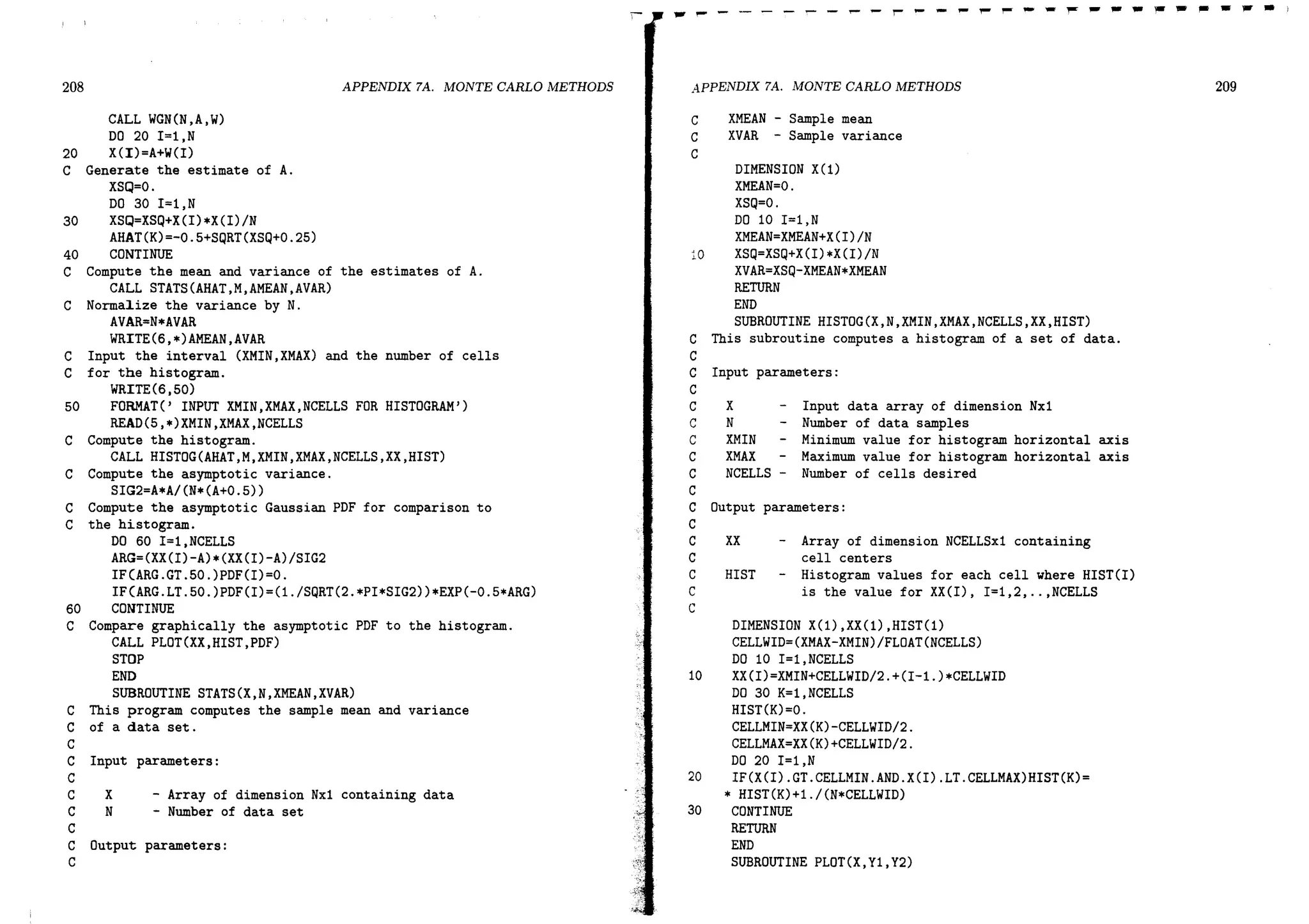
![210 APPENDIX 7A. MONTE CARLO METHODS
DIMENSION X(1),Yl(1),Y2(1)
C Replace this subroutine with any standard Fortran-compatible
C plotting routine.
RETURN
END
SUBROUTINE WGN(N,VAR,W)
C This subroutine generates samples of zero mean white
C Gaussian noise.
C
C Input parameters:
C
C N - Number of noise samples desired
C VAR - Variance of noise desired
C
C Output parameters:
C
C W - Array of dimension Nxl containing noise samples
C
DIMENSION W(l)
PI=4. *ATAN(1.)
C Add 1 to desired number of samples if N is odd.
Nl=N
IF(MOD(N,2).NE.0)Nl=N+l
C Generate Nl independent and uniformly distributed random
C variates on [0,1].
CALL RANDOM(Nl,VAR,W)
L=N1/2
C Convert uniformly distributed random variates to Gaussian
C ones using a Box-Mueller transformation.
DO 10 I=l,L
Ul=W(2*I-1)
U2=W(2*I)
TEMP=SQRT(-2.*ALOG(Ul))
W(2*I-l)=TEMP*COS(2.*PI*U2)*SQRT(VAR)
10 W(2*I)=TEMP*SIN(2.*PI*U2)*SQRT(VAR)
RETURN
END
SUBROUTINE RANDOM(Nl,VAR,W)
DIMENSION W(l)
DO 10 I=l,Nl
C For machines other than DEC VAX 11/780 replace RAN(ISEED)
C with a random number generator.
10 W(I)=RAN(lllll)
RETURN
END
.----- - - - - - - - - ~ ~ ~ ---- - .--...
Appendix 7B
Asymptotic PDF of MLE for a Scalar
Parameter
We now give an outline of the proof of Theorem 7.1. A rigorous proof of consistency
can be found in [Dudewicz 1976] and of the asymptotic Gaussian property in [Rao
1973]. To simplify the discussion the observations are assumed to be lID. We further
assume the following regularity conditions.
1. The first-order and second-order derivatives of the log-likelihood function are well
defined.
2.
We first show that the MLE is consistent. To do so we will need the following inequality
(see [Dudewicz 1976] for proof), which is related to the Kullback-Leibler information.
(7B.1)
with equality if and only if el = ()2. Now, in maximizing the log-likelihood function,
we are equivalently maximizing
1
N lnp(xi e)
1 N-I
N In II p(x[n]i e)
n=O
1 N-I
N L lnp(x[n];e).
n=O
But as N ~ 00, this converges to the expected value by the law of large numbers.
Hence, if eo denotes the true value of e, we have
1 N-I
N L lnp(x[n]i e) ~ Jlnp(x[n]i e)p(x[n]i eo) dx[n].
n=O
(7B.2)
211](https://image.slidesharecdn.com/fundamentalsofstatisticalsignalprocessing-estimationtheory-kay-230513154707-1f7652e0/75/Fundamentals-Of-Statistical-Signal-Processing-Estimation-Theory-Kay-pdf-111-2048.jpg)
![212 APPENDIX 7B. ASYMPTOTIC PDF OF MLE
However, from (7B.l)
JIn [p(x[nJ; ( 1)J p(x[nJ; (1) dx[nJ 2: JIn [p(x[nJ; ( 2 )J p(x[nJ; (1) dx[nJ.
The right-hand side of (7B:2) is therefore maximized for 8 = 80 , By a suitable continuity
argument, the left-hand sIde of (7B.2) or the normalized log-likelihood function must
also .be maximized for 8 = 80 or as N -+ 00, the MLE is 0= 80
. Thus, the MLE is
consIstent.
To derive the asymptotic PDF of the MLE we first use a Taylor expansion about
the true value of 8, which is 80 • Then, by the mean value theorem
8Inp(x;8) I = 8Inp(X;8)/ 82
In p(X;8)/ '
88 8=6 88 8=8
0
+ 882 8=8 (8 - (0 )
where 80 < {} < O. But
8Inp(X;8)/ =0
88 8=6
by the definition of the MLE, so that
0= 8Inp(x;8) I 8
2
Inp(x;8) I '
88 + 882 _(8 - (0 ),
8=80 8=8
(7B.3)
Now consider VN(O - (0 ), so that (7B.3) becomes
1 8Inp(X;8)/
../N(O - (0
) = TN 88 8-80
_~ 8
2
Inp(x; 8) /
N 882
8=8
(7BA)
Due to the lID assumption
1 8
2
Inp(x;8) I = ~ ~ 82
In p(x[nJ;8)/
N 88
2
8=8 N ~ 882 8=8
Since 80 < fj < 0, we must also have {} -+ 80 due to the consistency of the MLE. Hence,
~ ~I 8
2
Inp(x[nJ; 8) I
N ~ 882
n=O 8=80
1 8
2
Inp(x; 8) I
N 882 --+
8=8
-+ E[82Inp(~[nJ;8)1 ]
88 8=80
-i(80 )
-,...- - - - r - ~ ~ ~ ~ ~ - - - - • • • • • • • •
A.PPENDIX 7B. ASYMPTOTIC PDF OF MLE 213
where the last convergence is due to the law of large numbers. Also, the numerator
term is
_1_~ 8Inp(x[nJ;8) I
v'N ~ 88
n=O 8=80
Now
'n= 8Inp(x[nJ; 8) I
88 8=80
is a random variable, being a function of x[nJ. Additionally, since the x[nl's are lID,
so are the 'n's. By the central limit theorem the numerator term in (7BA) has a PDF
that converges to a Gaussian with mean
E[_I_I:18Inp~[nJ;8)1 1=0
v'N n=O 8=80
and variance
E [ ( ~ '~a
Inp~nJ;9)I.J'] ~ ~E [ (aInp~i"J;9))'I.J
= i(80 )
due to the independence of the random variables. We now resort to Slutsky's theorem
[Bickel and Doksum 1977], which says that if the sequence of random variables Xn has
the asymptotic PDF of the random variable x and the sequence of random variables
Yn converges to a constant c, then xn/Yn has the same asymptotic PDF as the random
variable x/c. In our case,
so that (7BA) becomes
or, equivalently,
or finally
x '" N(O, i(80 ))
Yn -+ c = i(80 )
'a ( 1)
8", N 80 , Ni(80
)](https://image.slidesharecdn.com/fundamentalsofstatisticalsignalprocessing-estimationtheory-kay-230513154707-1f7652e0/75/Fundamentals-Of-Statistical-Signal-Processing-Estimation-Theory-Kay-pdf-112-2048.jpg)
![J _________ - - - - - - - - - - _ - _____ _
Appendix 7C
Derivation of Conditional
Log-Likelihood for EM Algorithm
Example
From (7.51) we have, upon noting the independent data set assumption,
p
Inpy(y; 9) = 2)np(Yi; Bi )
i=l
p {I [1 N-1 ]}
Lin 2 Ii. exp --2
2 L (Yi[n]- cos 27rfin)2
i=1 (27rai ) 2 ai n=O
p 1 N-1
C - L 2a2 L (y;[n]- cos 27rfin)2
i=l 1, n=O
p 1 N-1 1
= g(y) + L 2" L (y;[n] cos 27rfin - - cos2
27rfin)
i=1 ai n=O 2
where c is a constant and g(y) does not depend on the frequencies. Making the ap-
proximation that "2:~:01 cos227rfin ~ N/2 for fi not near 0 or 1/2, we have
p 1 N-1
Inpy(y;9) =h(y) + L 2" LYi[n]cos27rfin
a
i=l t n=O
or letting Ci = [1 cos 27rfi ... cos 27rfi(N - l)]T, we have
p 1
Inpy(y; 9) = h(y) +L 2"c;Yi·
i=1 ai
214
(7C.1)
• • • • • - - - • • • • • • « • - • • • • • • • • • • •
..l.PPENDIX 7C. DERIVATION FOR EM ALGORITHM EXAMPLE 215
Concatenating the Ci'S and y;'s as
C=
we have
Inpy(y; 9) = h(y) +cT
y.
From (7.56) we write the conditional expectation as
U(9,9k ) = E[lnpy(y; 9)lx; 9k ]
= E(h(y)lx; 9k ) + cT
E(ylx; 9k ). (7C.2)
Since we wish to maximize U(9,9k ) with respect to 9, we can omit the expected value
of h(y) since it does not depend on 9. Now, y and x are jointly Gaussian since, from
(7.52),
p
x = LYi = [I I. .. I]y
i=l
where 1 is the N x N identity matrix and the transformation matrix is composed of
p identity matrices. Using the standard result for conditional expectations of jointly
Gaussian random vectors (see Appendix IDA), we have
E(ylx; 9k ) = E(y) +CyxC;;;(x - E(x)).
T;le means are given by
E(r) r~~1
p
E(x) LCi
i=1
while the covariance matrices are](https://image.slidesharecdn.com/fundamentalsofstatisticalsignalprocessing-estimationtheory-kay-230513154707-1f7652e0/75/Fundamentals-Of-Statistical-Signal-Processing-Estimation-Theory-Kay-pdf-113-2048.jpg)
![216 APPENDIX 7C. DERIVATION FOR EM ALGORITHM EXAMPLE
so that
or
i=1,2, ... ,p
where Ci is computed using (h. Note that E(Ydx; 9k ) can be thought of as an estimate
of the Yi[n] data set since, letting Yi = E(Yilx; 9k ),
Yi[n] =cos 27r!i.n + :; (x[n]- tcoS27r!ikn). (7C.3)
Using (7G2) and dropping the term that is independent of 9, we have
P
U'(9,9k ) = LC;Yi
i=l
_ _ _ _ _ _ _ _ _ _ _ _ _ _ • • • • • • • • • I •
APPENDIX 7C. DERIVATION FOR EM ALGORITHM EXAMPLE 217
which is maximized over 9 by maximizing each term in the sum separately or
(7C.4)
Finally, since the aT's are not unique, they can be chosen arbitrarily as long as (see
(7.53))
i=l
0r, equivalently,](https://image.slidesharecdn.com/fundamentalsofstatisticalsignalprocessing-estimationtheory-kay-230513154707-1f7652e0/75/Fundamentals-Of-Statistical-Signal-Processing-Estimation-Theory-Kay-pdf-114-2048.jpg)
![11&1,11&1&&&&&1..& ...... ..1.. . . . . . . . . -..___-
220
e
e
Noise
CHAPTER B. LEAST SQUARES
Model
inaccuracies
"----_ x[n]
(a) Data model
Error =e[n]
x[n]
(b) Least squares error
Figure 8.1 Least squares approach
available, then a sequential approach can be employed. It determines the least squ~res
estimator based on the estimate at the previous time and the new data. The equatIOns
(8.46)-(8.48) summarize the calculations required. At times the parameter .vector ~s
constrained, as in (8.50). In such a case the constrained least squares estimator IS
given by (8.52). Nonlinear least squares is discussed in Section ~.9. S?me ~e:h?ds .for
converting the problem to a linear one are described, followed by Iterative mlmmlzatlOn
approaches if this is not possible. The two methods that are generally used are the
Newton-Raphson iteration of (8.61) and the Gauss-Newton iteration of (8.62).
8.3 The Least Squares Approach
Our focus in determining a good estimator has been to find one that was unbiased and
had minimum variance. In choosing the variance as our measure of goodness we im-
plicitly sought to minimize the discrepancy (on the average) between our estim~t~ a~d
the true parameter value. In the least squares (LS) approach we attempt to mllllmize
the squared difference between the given data x[n] and the assumed signal or noi~ele~s
data. This is illustrated in Figure 8.1. The signal is generated by some model which III
turn depends upon our unknown parameter 8. The signal s[n] is purely det.erministic.
Due to observation noise or model inaccuracies we observe a perturbed version of s[n],
which we denote by x[n]. The least squares estimator (LSE) of 8 chooses the value that
•••••• II •• IIIIIIIIIIIII •• IIJ
B.3. THE LEAST SQUARES APPROACH 221
makes s[n] closest to the observed data x[n]. Closeness is measured by the LS error
criterion
N-I
J(8) = L (x[nJ - s[n])2 (8.1)
n=O
where the observation interval is assumed to be n = 0,1, ... , N -1, and the dependence
of J on 8 is via s[nJ. The value of 8 that minimizes J(8) is the LSE. Note that no
pm,babilistic as~umptions have been made about the data x[nJ. The method is equally
vahd for Gaussian as well as non-Gaussian noise. Of course, the performance of the
LSE will undoubtedly depend upon the properties of the corrupting noise as well as
any modeling errors. LSEs are usually applied in situations where a precise statistical
characterization of the data is unknown or where an optimal estimator cannot be found
or may be too complicated to apply in practice.
Example 8.1 - DC Level Signal
Assume that the signal model in Figure 8.1 is s[nJ = A and we observe x[nJ for n =
0,1, ... , N -1. Then, according to the LS approach, we can estimate A by minimizing
(8.1) or
N-I
J(A) = L (x[n]- A)2.
n=O
Differentiating with respect to A and setting the result equal to zero produces
1 N-I
NLx[nJ
n=O
or the sample mean estimator. Our familiar estimator, however, cannot be claimed to
be optimal in the MVU sense but only in that it minimizes the LS error. We know,
however, from our previous discussions that if x[nJ = A+w[nJ, where w[nJ is zero mean
WGN, then the LSE will also be the MVU estimator, but otherwise not. To underscore
the potential difficulties, consider what would happen if the noise were not zero mean.
Then, the sample mean estimator would actually be an estimator of A +E(w[n]) since
w[nJ could be written as
w[nJ = E(w[n]) +w'[nJ
where w'[nJ is zero mean noise. The data are more appropriately described by
x[nJ = A + E(w[n]) +w'[nJ.
It should be clear that in using this approach, it must be assumed that the observed
data are composed of a deterministic signal and zero mean noise. If this is the case,
the error f[nJ = x[nJ- s[nJ will tend to be zero on the average for the correct choice of
the signal parameters. The minimization of (8.1) is then a reasonable approach. The
reader might also consider what would happen if the assumed DC level signal model](https://image.slidesharecdn.com/fundamentalsofstatisticalsignalprocessing-estimationtheory-kay-230513154707-1f7652e0/75/Fundamentals-Of-Statistical-Signal-Processing-Estimation-Theory-Kay-pdf-116-2048.jpg)
![4AA&A&I&&II&I&~.II •••••••••
222 CHAPTER 8. LEAST SQUARES
were incorrect, as for instance if x[nJ = A+Bn+w[nJ described the data. This modeling
error would also cause the LSE to be biased. <>
Example 8.2 - Sinusoidal Frequency Estimation
Consider the signal model
s[nJ = cos 27rfon
in which the frequency fo is to be estimated. The LSE is found by minimizing
N-l
J(/o) = z)x[nJ- cos 27rfon)2.
n=Q
In contrast to the DC level signal for which the minimum is easily found, here the LS
error is highly nonlinear in fo. The minimization cannot be done in closed form. Since
the error criterion is a quadratic function of the signal, a signal that is linear in the
unknown parameter yields a quadratic function for J, as in the previous example. The
minimization is then easily carried out. A signal model that is linear in the unknown
parameter is said to generate a linear least squares problem. Otherwise, as in this
example, the problem is a nonlinear least squares problem. Nonlinear LS problems are
solved via grid searches or iterative minimization methods as described in Section 8.9.
It should be noted that the signal itself need not be linear but only in the unknown
parameter, as the next example illustrates. <>
Example 8.3 - Sinusoidal Amplitude Estimation
If the signal is s[nJ = A cos 27rfon, where fo is known and A is to be estimated, then
the LSE minimizes
N-l
J(A) = z)x[nJ- Acos 27rfon?
n=O
over A. This is easily accomplished by differentiation since J(A) is quadratic in A. This
linear LS problem is clearly very desirable from a practical viewpoint. If, however, A
were known and the frequency were to be estimated, the problem would be equivalent
to that in Example 8.2, that is to say, it would be a nonlinear LS problem. A final
possibility, in the vector parameter case, is that both A and fo might need to be
estimated. Then, the error criterion
N-l
J(A,fo) = L(x[nJ-Acos27rfon)2
n=O
is quadratic in A but nonquadratic in fo. The net result is that J can be minimized
in closed form with respect to A for a given fo, reducing the minimization of J to one
8.4. LINEAR LEAST SQUARES
223
over fo ~nly. :rhis type .of problem, in which the signal is linear in some parameters
b~t n?nhnear ~n others, IS termed a separable least squares problem. In Section 8 9
~~~~~her .~
. <>
8.4 Linear Least Squares
In applying the linear LS approach for a scalar parameter we must assume that
s[nJ = Oh[nJ (8.2)
~here h[nJ is a known s~quence. (The reader may want to refer back to Chapter 6 on
t e BLUE for a companson to similar signal models.) The LS error criterion becomes
N-I
J(O) = L (x[nJ- Oh[nJ?
n=O
A minimization is readily shown to produce the LSE
N-l
Lx[nJh[nJ
n=O
The minimum LS error, obtained by substituting (8.4) into (8.3), is
N-I
Jrnin = J(8) = L (x[nJ- 8h[n])(x[nJ- 8h[n])
n=O
N-I N-I
L x[n](x[nJ - 8h[n]) - 8L h[n](x[nJ- 8h[n])
n=O n=O
'---..
...-----"
S
N-I N-I
L x
2
[nJ - 8L x[nJh[nJ.
n=O n=O
(8.3)
(8.4)
(8.5)
The l?-Bt step follows because the sum S is zero (substitute 8to verify). Alternatively,
by usmg (8.4) we can rewrite Jrnin as
(8.6)
n=O](https://image.slidesharecdn.com/fundamentalsofstatisticalsignalprocessing-estimationtheory-kay-230513154707-1f7652e0/75/Fundamentals-Of-Statistical-Signal-Processing-Estimation-Theory-Kay-pdf-117-2048.jpg)
![224
CHAPTER 8. LEAST SQUARES
The minimum LS error is the original energy of the data or L~:OI x
2
[nJ less that due
to the signal fitting. For Example 8.1 in which () = A we have h[nJ = 1, so that from
(8.4) A=x and from (8.5)
N-I
Jrnin = L x2[nJ - Nx
2
.
n=O
If the data were noiseless so that x[nJ = A, then Jrnin = 0 or we would have a perfect
LS fit to the data. On the other hand, if x[nJ = A + w[nJ, where E(w
2
[nJ) »A2, then
L~:OI x2 [nJlN» x2 • The minimum LS error would then be
N-I
Jrnin ::::: L x
2
[nJ
n=O
)
or not much different than the original error. It can be shown (see Problem 8.2) that
the minimum LS error is always between these two extremes or
N-I
os: Jrnin s: L x
2
[nJ. (8.7)
n=O
The extension of these results to a vector parameter 9 of dimension p x 1 is straight-
forward and of great practical utility. For the signal s = [s[OJ s[lJ ... s[N - 1]jT to be
linear in the unknown parameters, we assume, using matrix notation,
s=H9 (8.8)
where H is a known N x p matrix (N > p) of full rank p. The matrix H is referred to
as the obsenJation matrix. This is, of course, the linear model, albeit without the usual
noise PDF assumption. Many examples of signals satisfying this model can be found
in Chapter 4. The LSE is found by minimizing
N-I
J(9) L (x[nJ - s[nJ)2
(x - H9f(x - H9). (8.9)
This is easily accomplished (since J is a quadratic function of 9) by using (4.3). Since
J(9) xT X - xTH9 - 9THTx +9THTH9
xT x - 2xTH9 +9THTH9
(note that x T H9 is a scalar), the gradient is
~ _____ ~ __ ~ __ • • • • • • • • • I I I . I I •• J
8.4. LINEAR LEAST SQUARES 225
Setting the gradient equal to zero yields the LSE
(8.10)
The equations HTH9 = HTx to be solved for iJ are termed the normal equations.
The assumed full rank of H guarantees the invertibility of HTH. See also Problem
8.4 for another derivation. Somewhat surprisingly, we obtain an estimator that has
the identical funct~onal form as the efficient estimator for the linear model as well as
the BLUE. That 9 as given by (8.10) is not the identical estimator stems from the
assumptions made about the data. For it to be the BLUE would require E(x) = H9
and ~x = a 2
1 (see Ch~pter 6), and to be efficient would in addition to these properties
reqUire x t.o be Gaussian (see Chapter 4). As a side issue, if these assumptions hold
we can. easl~y determine the statistical properties of the LSE (see Problem 8.6), havin~
been given In Chapters 4 and 6. Otherwise, this may be quite difficult. The minimum
LS error is found from (8.9) and (8.10) as
J(iJ)
(x - HiJf(x - HiJ)
(x - H(HTH)-IHTX)T (x - H(HTH)-IHTx)
xT (I - H(HTH)-IHT) (I - H(HTH)-IHT) x
xT (I - H(HTH)-IHT) x. (8.11)
The last step results from the fact that 1 - H(HTH)-I HT is an idempotent matrix or
it has the property A2
= A. Other forms for Jrnin are
xTX - xTH(HTH)-IHTX
xT(x - HiJ).
(8.12)
(8.13)
;n extension of the li~:ar LS p~oblem is to weighted LS. Instead of minimizing (8.9),
we In.elude an N x N posItive defimte (and by definition therefore symmetric) weighting
matnx W, so that
J(9) = (x - H9fW(x - H9). (8.14)
If, for instance, W is diagonal with diagonal elements [WJii = Wi > 0, then the LS error
for Example 8.1 will be
N-I
J(A) = L wn(x[n]- A)2.
n=O
The ratio~ale. for introducing weighting factors into the error criterion is to emphasize
the ?ont:lbutlOns of thos: data samples that are deemed to be more reliable. Again,
conSiderIng Example 8.1, If x[n] = A+w[n], where w[n] is zero mean uncorrelated noise
with variance a~, then it is reasonable to choose Wn = l/a~. This choice will result in](https://image.slidesharecdn.com/fundamentalsofstatisticalsignalprocessing-estimationtheory-kay-230513154707-1f7652e0/75/Fundamentals-Of-Statistical-Signal-Processing-Estimation-Theory-Kay-pdf-118-2048.jpg)
![.....-....•....... -~------~-.
226 CHAPTER B. LEAST SQUARES
the estimator (see Problem 8.8)
f x[~]
A -0 an
A= n_ .
N-1 1
L a2
n=O n
(8.15)
This familiar estimator is of course the BLUE since the w[nl's are uncorrelated so that
W = C-1 (see Example 6.2).
The general form of the weighted LSE is readily shown to be
(8.16)
and its minimum LS error is
(8.17)
(see Problem 8.9).
8.5 Geometrical Interpretations
We now reexamine the linear LS approach from a geometrical perspective. This has the
advantage of more clearly revealing the essence of the approach and leads to additional
useful properties and insights into the estimator. Recall the general signal model s =
H9. If we denote the columns of H by hi, we have
p
LB;h;
i=l
so that the signal model is seen to be a linear combination of the "signal" vectors
{hI> h2, ••• , hp}.
Example 8.4 - Fourier Analysis
Referring to Example 4.2 (with M = 1), we suppose the signal model to be
s[n] = a cos 27rfon +bsin27rfon n = 0, 1, ... , N - 1
B.5. GEOMETRICAL INTERPRETATIONS 227
where fo is a known frequency and 9 = [a bJT is to be estimated. Then, in vector form
we have
[
s[O] 1
s[l]
s[N:-1]
(8.18)
It is seen that the columns of H are composed of the samples of the cosinusoidal and
sinusoidal sequences. Alternatively, since
we have
[1 cos 27rfo
[0 sin 27rfo
The LS error was defined to be
cos 27rfo(N - 1) ]T
sin 27rJo(N - 1) (,
J(9) = (x - H9)T(X - H9).
o
If we further define the Euclidean length of an N x 1 vector e= [6 6 ... ~NJT as
then the LS error can be also written as
J(9) Ilx-H9W
p
Ilx - LBi hil1
2
• (8.19)
i=l
We now see that the linear LS approach attempts to minimize the square of the distance
from the data vector x to a signal vector L:f=1 Bih;, which must be a linear combination
of the columns of H. The data vector can lie anywhere in an N-dimensional space,
termed RN, while all possible signal vectors, being linear combinations ofp < N vectors,
must lie in a p-dimensional subspace of RN, termed SP. (The full rank of H assumption
assures us that the columns are linearly independent and hence the subspace spanned
is truly p-dimensional.) For N = 3 and p = 2 we illustrate this in Figure 8.2. Note
that all possible choices of B}, B2 (where we assume -00 < B1 < 00 and -00 < B2 < 00)
produce signal vectors constrained to lie in the subspace S2 and that in general x does
not lie in the subspace. It should be intuitively clear that the vector sthat lies in S2 and](https://image.slidesharecdn.com/fundamentalsofstatisticalsignalprocessing-estimationtheory-kay-230513154707-1f7652e0/75/Fundamentals-Of-Statistical-Signal-Processing-Estimation-Theory-Kay-pdf-119-2048.jpg)
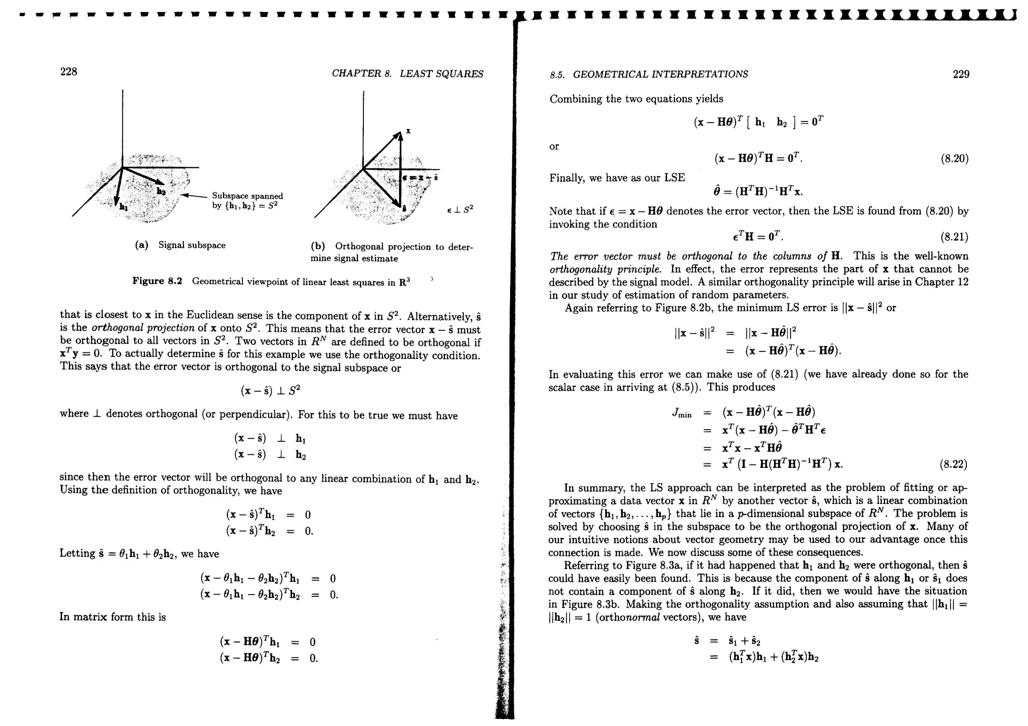
![~-- - - ,- ~ r
230 CHAPTER 8. LEAST SQUARES
x
(a) Orthogonal hi'S
(b) Nonorthogonal h;'s
Figure 8.3 Effect of nonorthogonal columns of observation matrix
where hTx is the length of the vector x along 11;. In matrix notation this is
so that
s [hI hz] [ :~: ]
[hI hz] [ :~ ] x
HHTx
This result is due to the orthonormal columns of H. As a result, we have
and therefore
No inversion is necessary. An example follows.
Example 8.5 - Fourier Analysis (continued)
Continuing Example 8.4, if fo = kiN, where k is an integer taking on any of the values
k =1,2, ... ,N12 -1, it is easily shown (see (4.13)) that
8.5. GEOMETRICAL INTERPRETATIONS
and also
N
2
N
2
231
so that hI and h2 are orthogonal but not orthonormal. Combining these results produces
HTH = (NI2)I, and therefore,
If we had instead defined the signal as
s[nJ = a' ~cos ( 27r ~n) +b'~sin (27r ~n)
then the columns of H would have been orthonormal. o
In general, the columns of H will not be orthogonal, so that the signal vector estimate
is obtained as
s= HB = H(HTH)-IHTx.
The signal estimate is the orthogonal projection of x onto the p-dimensional subspace.
The N x N matrix P = H (HTH) -IHT is known as the orthogonal projection matrix or
just the projection matrix. It has the properties
1. pT
= P, symmetric
2. p2 = P, idempotent.
That the projection matrix must be symmetric is shown in Problem 8.11, that it must be
idempotent follows from the observation that if P is applied to Px, then the same vector
must result since Px is already in the subspace. Additionally, the projection matrix
must be singular (for independent columns of H it has rank p, as shown in Problem
8.12). If it were not, then x could be recovered from s, which is clearly impossible since
many x's have the same projection, as shown in Figure 8.4.](https://image.slidesharecdn.com/fundamentalsofstatisticalsignalprocessing-estimationtheory-kay-230513154707-1f7652e0/75/Fundamentals-Of-Statistical-Signal-Processing-Estimation-Theory-Kay-pdf-121-2048.jpg)
![,...........•......•..•••....
232 CHAPTER 8. LEAST SQUARES
Figure 8.4 Vectors with same
projection onto subspace
Likewise, the error vector 10 = X - S = (I - P)x is the projection of x onto the
complement subspace or the subspace orthogonal to the signal subspace. The matrix
pl. = 1 _ P is also a projection matrix, as can be easily verified from the properties
given above. As a result, the minimum L8 error is, from (8.22),
Jrnin xT
(I - P)x
xTpl.x
XTpl.Tpl. X
IIPJ.xW
which is just IleW.
In th.e next section we further utilize the geometrical theory to derive an order-
recursive L8 solution.
8.6 Order-Recursive Least Squares
In many cases the signal model is unknown and must be assumed. For example, consider
the experimental data shown in Figure 8.5a. The following models might be assumed
81 (t) A
82(t) = A + Bt
for 0:::; t :::; T. If data x[n] are obtained by sampling x(t) at times t = n~, where ~ = 1
and n = 0,1, ... , N - 1, the corresponding discrete-time signal models become
Using a L8E with
A
A+Bn.
[:1 H2 = [ : : 1
l I N -1
5.0 -
4.5 -
4.0..,
3.5..,
3.0 -
2.5 -
2.0 -
1.5 _
....-
1.0 - o·
0.5.
0.0 I
0
5.0 -c
4.5 -
4.0 _
3.5 -
3.0 -
2.5
2.0 -
1.5 _
....-
1.0 -
0.5.
0.0 I
0
5.0 -
4.5 -
4.0 -
3.5..,
3.0..,
2.5.;
2.0 J
1.0
0.5.
0
00
0
0
10
0
00
0
10
(a) Experimental data
.' . .'
.
..
.
.
'., '. 00
20 30 40 50 60
Time, t
(b) One-parameter fit
0
0 000
0
00
o •
. 00
00
0
0
000
00 000
0
20 30 40 50 60
Time, t
(c) Two-parameter fit
.
.'
. .
.. . .
. . .
.
.
.'
' .
70 80 90 100
0
00
0 0
0
0
0
00
'0 0
..
00
'
SI(t) = Al
70 80 90 100
00
0.0 +1--r----r----r---"T--r-----r-----r-----,---r--~
o 10 20 30 40 50 60 70 80 90 100
Time, t
Figure 8.5 Experimental data fitting by least squares](https://image.slidesharecdn.com/fundamentalsofstatisticalsignalprocessing-estimationtheory-kay-230513154707-1f7652e0/75/Fundamentals-Of-Statistical-Signal-Processing-Estimation-Theory-Kay-pdf-122-2048.jpg)
![L....a..&.,~ ____ .& . . . . . . . . . . . . . . . . . . . . . . . .
234 CHAPTER 8. LEAST SQUARES
"
~
100
90
80
70
60~
50
1
40
~ Constant
Parabola Cubic
I
Line
~~~ I I
~-;-----I----:
I
1~1 I : I
1.0 1.5 2.0 2.5 3.0 3.5 4.0
Number of parameters, k
Figure 8.6 Effect of chosen number of parameters on minimum least
squares error
would produce the estimates for the intercept and slope as
Al = x
and (see Problem 8.13)
2(2N - 1) N-l 6 N-l
N(N +1) ~ x[n] - N(N + 1) ~ nx[n]
6 N-l 12 N-l
N(N + 1) ~ x[n] + N(N2 _ 1) ~ nx[n].
(8.23)
(8.24)
In Figures 8.5b and 8.5c we have plotted SI(t) = Al and S2(t) = A2 + iht, where
T = 100. The fit using two parameters is better, as expected. We will later show that
the minimum LS error must decrease as we add more parameters. The question might
be asked whether or not we should add a quadratic term to the signal model. If we
did, the fit would become better yet. Realizing that the data are subject to error, we
may very well be jitting the noise. Such a situation is undesirable but in the absence of
a known signal model may be unavoidable to some extent. In practice, we choose the
simplest signal model that adequately describes the data. One such scheme might be to
increase the order of the polynomial until the minimum LS error decreases only slightly
as the order is increased. For the data in Figure 8.5 the minimum LS error versus
the number of parameters is shown in Figure 8.6. Models SI(t) and S2(t) correspond
to k = 1 and k = 2, respectively. It is seen that a large drop occurs at k = 2. For
larger orders there is only a slight decrease, indicating a modeling of the noise. In this
example the signal was actually
s(t) = 1 +0.03t
• ••• •••••• III.II ••••••• IIII.)
8.6. ORDER-RECURSIVE LEAST SQUARES
235
an~ the noise win] was WGN with variance (]'z = 0.1. Note that if A, B had been
estImated perfectly, the minimum LS error would have been
Jrnin J(A, B)
J(A, B)
N-l
L (x[n] - sin]?
n=O
n=O
~ N(]'Z
so t~at when the true order is reached, Jrnin ~ 10. This is verified in Figure 8.6 and
also Increases our confidence in the chosen model.
In the preced~ng example we saw that it was important to be able to determine the
LSE for severa! signal models. A straightforward approach would compute the LSE for
each model USIng (8.10). Alternati.vely, the computation may be reduced by using an
order-recurswe LS approach. In thiS method we update the LSE . d S 'fi 11
bl In or er. peci ca y
we a:e a e to compute the. LSE based on an H of dimension N x (k + 1) from th~
solutIOn based on an H of dimension N x k. For the previous example this update in
order would have bee~ exceedingly simple had the columns of H2 been orthogonal. To
see why assume the signal models to be
sl[n] = Al
sz[n] = A2 +B2n
~or -M :S n :S M. We have now altered the observation interval to be the symmetric
Interval .r-"':1, M] as oppos~d to the original [0, N - 1] interval. The effect of this
assumptIOn IS to orthogonahze the columns of Hz since now
H, ~ [; -(7)]
The LSE is readily found since
[
2M +1
HfHz= 0
is a diagonal matrix. The solutions are
_ 1 M
A1 = - - L x[n]
2M + 1 n=-M](https://image.slidesharecdn.com/fundamentalsofstatisticalsignalprocessing-estimationtheory-kay-230513154707-1f7652e0/75/Fundamentals-Of-Statistical-Signal-Processing-Estimation-Theory-Kay-pdf-123-2048.jpg)
![,'IIAAI.I'AA'A"I"AA •• '.1••
236
hi
and
Projection of h2
h~
"
hi .1 h~
CHAPTER 8. LEAST SQUARES
Figure 8.7 Gram-Schmidt
orthogonalization
1 M
2M+1 L x[n]
n=-M
M
L nx[n]
n=-lvl
In this case the LSE of A does not change as we add a parameter to the model and
follows algebraically from the diagonal nature of HIH2. In geometric terms this result
is readily apparent from Figure 8.3a. The orthogonality of the h;'s allows us to project
x along hi and h2 separately and then add the results. Each projection is independent
of the other. In general, the column vectors will not be orthogonal but can be replaced
by anoth.er set of p vectors that are orthogonal. The procedure for doing so is shown
in Figure 8.7 and is called a Gram-Schmidt orthogonalization. The new column h2 is
projected onto the subspace orthogonal to hi' Then, since hi and h~ are orthogonal,
the LS signal estimate becomes
s= hlel +h~e;
where hlel is also the LSE for the signal based on H = hi only. This procedure
recursively adds terms to the signal model; it updates the order. In Problem 8.14
this geometrical viewpoint is used together with a Gram-Schmidt orthogonalization to
derive the order-update equations. A purely algebraic derivation is given in Appendix
8A. It is now summarized.
Denote the N x k observation matrix as Hk, and the LSE based on Hk as {h or
(8.25)
The minimum LS error based on Hk is
(8.26)
~____ • • • I . I . I I . I I I I . I I I I I I I I IIIIJ
8.6. ORDER-RECURSIVE LEAST SQUARES 237
By increasing the order to k + 1 we add a column to the observation m t' Thl's
t b ' a rlX.
genera es a new 0 servatlOn matrix which in partitioned form is
Hk+1 = [Hk hk+1 1= [ N x k N x 1 1. (8.27)
To update {h and Jmin• we use
=[kX1]
1 x 1
(8.28)
where
pt = I - Hk(H[Hk)-IH[
is the projection matrix onto the subspace orthogonal to that spanned by th I
f H
.,., 'd . . HT e co umns
o k'.LO avO! mvertmg kHk we let
(8.29)
(8.30)
J. - J (hk+1Ptx)
2
mm.+! - min. - hT Pl.h . (8.31)
k+1 k k+1
Ihe entire algorithm.requires no matrix inversions. The recursion begins by determining
01, Jmin" and DI usmg (8.25), (8.26), and (8.29), respectively. We term (8.28), (8.30),
:md (8.31) the order-recursive least squares method. To illustrate the computations
mvolved we apply the method to the previous line fitting example.
Example 8.6 - Line Fitting
Since sl[n] = Al and s2[n] = A2 + B2n for n = 0,1, ... , N - 1, we have](https://image.slidesharecdn.com/fundamentalsofstatisticalsignalprocessing-estimationtheory-kay-230513154707-1f7652e0/75/Fundamentals-Of-Statistical-Signal-Processing-Estimation-Theory-Kay-pdf-124-2048.jpg)
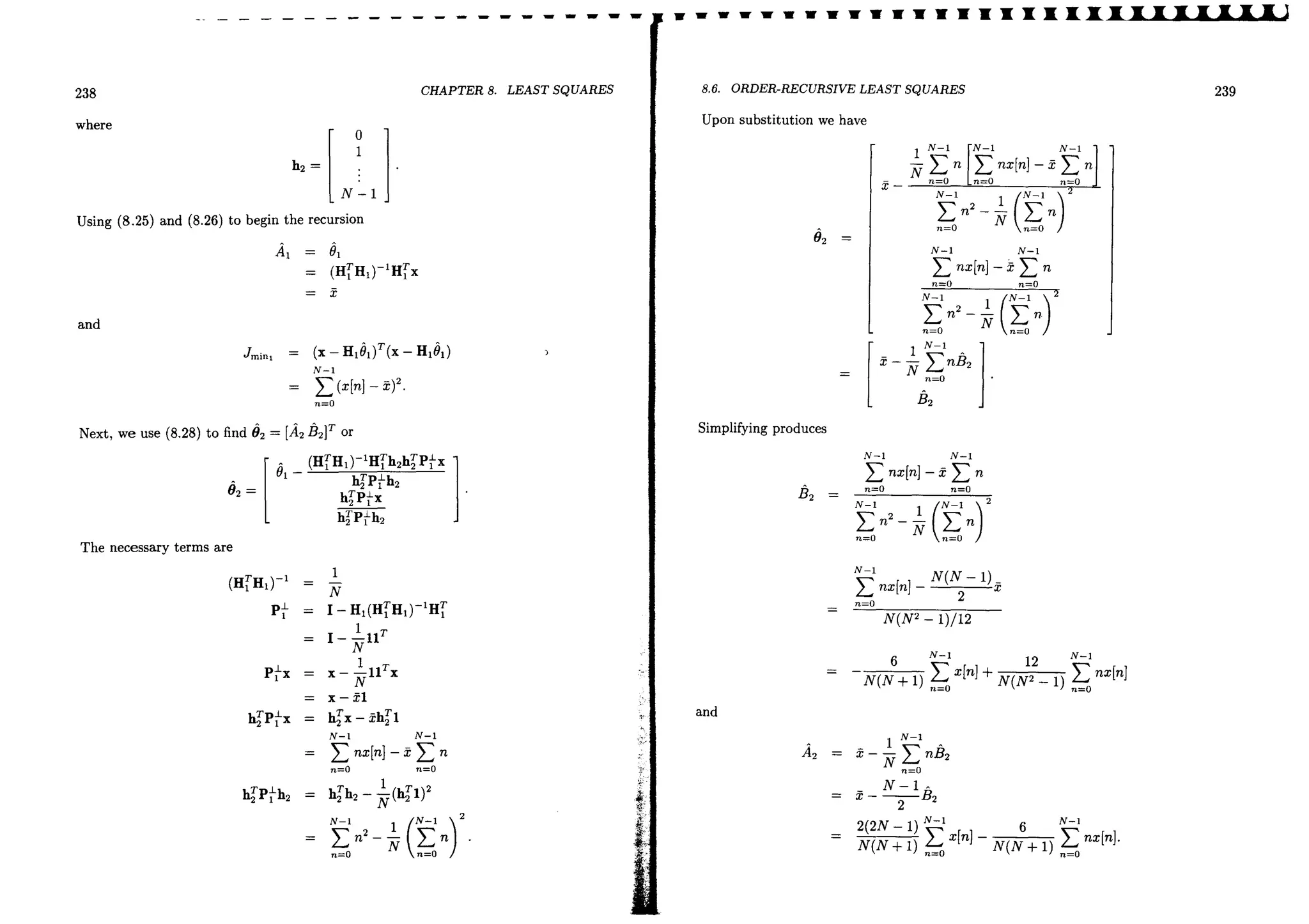
![240 CHAPTER 8. LEAST SQUARES
These are seen to agree with (8.24). The minimum LS error is, from (8.31),
(hfPtX)2
Jmin1
- hIPth2
(~nx[n]-x~n)'
J
mm
, - ~n' - ~ (~nr
(
N-I N )2
?;nx[n]- "2(N - l)x
Jmin,
- N(N2 - 1)/12
<>
In solving for the LSE of the parameters of the second-order model we first solved ~or
the LSE of the first-order model. In general, the recursive procedure solves successIve
LS problems until the desired order is attained. Hence, the recursive order~update
solution not only determines the LSE for the desired model but also determmes the
LSE for all lower-order models as well. As discussed previously, this property is useful
when the model order is not known a priori.
Several interesting observations can be made based on (8.28).
1. If the new column hk+I is orthogonal to all the previous ones, then HIhk+I = 0 and
from (8.28)
or the LSE for the first k components of 9k+1 remains the same. This generalizes
the geometrical illustration in Figure 8.3a.
2. The term Ptx = (I - Hk(HIHk)-IHI)x = x - Hk9k = €k is the LS error vector
or the data residual that cannot be modeled by the columns of Hk • It represents
the component of x orthogonal to the space spanned by the columns of Hk (see
Problem 8.17). We can view Ptx, the residual, as the part ofx yet to be modeled.
3. If hk+1 is nearly in the space spanned by the columns of Hk , then, as shown in
Figure 8.8, Pthk+I will be small. Consequently,
T.1 T p.1Tp.1h
hk+Ip k hk+I hk+I k k k+1
IIPthk+IW
~ 0
_---- •••••• IIIIIIIIIIIIIIIIIJ
8.6. ORDER-RECURSIVE LEAST SQUARES 241
= new information in hk+1
Figure 8.8 Near collinearity of columns of observation matrix
and the recursive procedure will "blow up" (see (8.28». In essence, since hk+1
nearly lies in the subspace spanned by the columns of Hk , the new observation
matrix Hk+I will be nearly of rank k and hence HI+!Hk+! will be nearly singular.
In practice, we could monitor the term hI+Ipthk+I and exclude from the recursion
those column vectors that produce small values of this term.
4. The minimum LS error can also be written in a more suggestive fashion, indicating
the contribution of the new parameter in reducing the error. From (8.22) and
(8.31) we have
xT p.1X
_ (hI+IPtX)2
k hk+IPthk+I
xT p.1X [1 _ (hk+!Ptx)
2
]
k xTPtxhk+!Pthk+!
Jmin.(1 - r~+I) (8.32)
where
2 [(Pthk+IY(PtX)]
2
rk+I = IIPt hk+IWIIPtxI12 · (8.33)
Letting (x,y) = xTy denote the inner product in RN , we have
where r~+I is seen to be the square of a correlation coefficient and as such has the
property](https://image.slidesharecdn.com/fundamentalsofstatisticalsignalprocessing-estimationtheory-kay-230513154707-1f7652e0/75/Fundamentals-Of-Statistical-Signal-Processing-Estimation-Theory-Kay-pdf-126-2048.jpg)
![242 CHAPTER 8. LEAST SQUARES
Intuitively, ptx represents the residual or error in modeling x based on k pa-
rameters, while pthk+1 represents the new model information contributed by
the (k + l)st parameter (see Figure 8.8). For instance, if ptx and Pthk+l are
collinear, then r~+1 = 1 and Jrnink+l = O. This says that the part of x that could
not be modeled by the columns of Hk can be perfectly modeled by hk+1' Assum-
ing that rk+l i= 0, the expression of (8.32) also shows that the minimum LS error
monotonically decreases with order as in Figure 8.6.
5. Recall that the LS signal estimate is
s= HO = Px
where P is the projection matrix. It is shown in Appendix 8B that P may be
recursively updated by using (8.28). The result is
(8.34)
This is termed the recursive orthogonal projection matrix. See Problem 8.18 for
its utility in determining the recursive formula for the minimum LS error. If we
define the unit length vector
(I - Pk )hk +1
11(1 - Pk)hk+111
Pthk+1
IIPthk+111
the recursive projection operator becomes
Pk+1 = Pk +uk+1uI+1
where Uk+1 points in the direction of the new information (see Figure 8.8), or by
letting Sk = PkX, we have
Sk+1 Pk+1X
Pkx + (uI+1X)Uk+1
Sk + (UI+1X)Uk+1'
8.7 Sequential Least Squares
In many signal processing applications the received data are obtained by sampling a
continuous-time waveform. Such data are on-going in that as time progresses, more
data become available. We have the option of either waiting for all the available data
or, as we now describe, of processing the data sequentially in time. This yields a
sequence of LSEs in time. Specifically, assume we have determined the LSE {J based on
8.7. SEQUENTIAL LEAST SQUARES 243
{x[~], x[I]' ... ,x[N -l)}. If we n?w observe x[N], can we update {J (in time) without
~avmg to resolve the lmear equatIOns of (8.1O)? The answer is yes, and the procedure
IS termed sequentzal least squares to distinguish it from our original approach in which
we processed all the data at once, termed the batch approach.
Consider Example 8.1 in which the DC signal level is to be estimated. We saw that
the LSE is
1 N-l
A[N-l]= N Lx[n]
n=O
where the argument of Adenotes the index of the most recent data point observed. If
we now observe the new data sample x[N], then the LSE becomes
A 1 N
A[N] = N+l Lx[n].
n=O
In computing this new estimator we do not have to recompute the sum of the observa-
tions since
1 (N-l )
A[N] N + 1 ~ x[n] + x[N]
N A 1
= N + 1A[N -1] + N + 1x[N]. (8.35)
~he new LSE is found by using the previous one and the new observation. The sequen-
tIal approach also lends itself to an interesting interpretation. Rearranging (8.35), we
have
A[N]=A[N-l]+ N~1 (x[N]-A[N-l]). (8.36)
The new estimate is equal to the old one plus a correction term. The correction term
decreases with N, reflecting the fact that the estimate A[N - 1] is based on many
more data samples and therefor.e shoul? ?e given more weight. Also, x[N] - A[N - 1]
can be thought of as the error m predIctmg x[N] by the previous samples, which are
summarized by A[N - 1]. If this error is zero, then no correction takes place for that
update. Otherwise, the new estimate differs from the old one.
The minimum LS error may also be computed recursively. Based on data samples
up to time N - 1, the error is
N-l
Jrnin[N - 1] = L (x[n]- A[N - 1])2
n=O
and thus using (8.36)
N
L(x[n]- A[N])2
n=O](https://image.slidesharecdn.com/fundamentalsofstatisticalsignalprocessing-estimationtheory-kay-230513154707-1f7652e0/75/Fundamentals-Of-Statistical-Signal-Processing-Estimation-Theory-Kay-pdf-127-2048.jpg)
![--------------------....
244 CHAPTER 8. LEAST SQUARES
N-l[ 1 ]2
~ x[n]- A[N - 1] - N + 1(x[N]- A[N - 1]) + (x[N] - A[N])2
2 N-l
Jmin[N - 1] - ~ L (x[n]- A[N - l])(x[N] - A[N - 1])
+ 1 n=O
N - -
+ (N + 1)2 (x[N]- A[N _1])2 + (x[N]- A[N])2.
Noting that the middle term on the right-hand side is zero, we have after some simpli-
cation
] [
N - 2
Jmin[N = Jmin N - 1] + N + 1(x[N]- A[N - 1]) .
The apparent paradoxical behavior of an increase in the minimum LS error is readily
explained if we note that with each new data point, the number of squared error terms
increases. Thus, we need to fit more points with the same number of parameters.
A more interesting example of a sequential LS approach arises in the weighted LS
problem. For the present example, if the weighting matrix W is diagonal, with [W]ii =
l/(jr, then the weighted LSE is, from (8.15),
To find the sequential version
A[N]
~ x[n]
L 172
A[N _ 1] = n=O n
N-l 1
t x[n]
n=O (j~
N 1
L 172
n=O n
L 172
n=O n
(
N-l 1 )
L 172
A[N -1] x[~]
n=O n +~
N 1 N 1
L 172 L 172
n=O n n=O n
. . . 1f 1f ...................... I I .... I I IIIIII..I.J
8.7. SEQUENTIAL LEAST SQUARES 245
_1A[N _ 1] x[N]
172 172
A[N-1]- N +_N_
N 1 N 1
L 172 L 172
n==O n n=O n
or finally
1
- - ';? -
A[N] = A[N - 1] + ~(x[N] - A[N - 1]).
1
L 172
n=O n
(8.37)
As expected, if (j~ = 172
for all n, we have our previous result. The gain factor that
multiplies the correction term now depends on our confidence in the new data sample.
If the new sample is noisy or (jJv -+ 00, we do not correct the previous LSE. On the
other hand, if the new sample is noise-free or (jJv -+ 0, then A[N] -+ x[N]. We discard
all the previous samples. The gain factor then represents our confidence in the new
data sample relative to the previous ones. We can make a further interpretation of
our results if indeed x[n] = A +w[n], where w[n] is zero mean uncorrelated noise with
variance 17;. Then, we know from Chapter 6 (see Example 6.2) that the LSE is actually
the BLUE, and therefore,
- 1
var(A[N - 1]) = ~
1
L 172
n=O n
and the gain factor for the Nth correction is (see (8.37»
K[N]
1
';?
_N_
N 1
L 172
n=O n
1
(jJv
1 1
-2- + -
(jN var(A[N - 1])
var(A[N - 1])
var(A[N - 1]) +(jJv
(8.38)
Since 0 ::; K[N] ::; 1, the correction is large if K[N] is large or var(A[N - 1]) is large.
Likewise, if the variance of the previous estimator is small, then so is the correction.
Further expressions may be developed for determining the gain recursively, since K[N]](https://image.slidesharecdn.com/fundamentalsofstatisticalsignalprocessing-estimationtheory-kay-230513154707-1f7652e0/75/Fundamentals-Of-Statistical-Signal-Processing-Estimation-Theory-Kay-pdf-128-2048.jpg)
![----~-------------
246 CHAPTER 8. LEAST SQUARES
depends on var(A[N - 1]). We can express the latter as
or finally
var(A[N]) =
1
N 1
L 0'2
n=O n
1
N-J 1 1
L 0'2 +;;:z
n=O n N
1
1 1
, + -2-
var(A[N - 1]) O'N
var(A[N - 1])0'~
var(A[N - 1]) +O'~
(
1 _ va:(A[N - 1]) ) var(A[N - 1])
var(A[N - 1]) + O'~
var(A[N]) = (1 - K[N])var(A[N - 1]). (8.39)
To find K[N] recursively we can use (8.38) and (8.39) as summarized below. In the
process of recursively finding the gain, the variance of the LSE is also found recursively.
Summarizing our results, we have
Estimator Update:
where
Variance Update:
A[N] = A[N - 1] +K[N](x[N]- A[N - 1])
K[N] = va:(A[N - 1])
var(A[N - 1]) +O'~
var(A[N]) = (1 - K[N])var(A[N - 1]).
To start the recursion we use
..1[0] x[O]
var(A[O]) O'~.
(8.40)
(8.41)
(8.42)
Then, K[I] is found from (8.41), and ..1[1] from (8.40). Next, var(A[I]) is determined
from (8.42). Continuing in this manner, we find K[2], A[2], var(A[2]), etc. An example
of the sequential LS approach is shown in Figure 8.9 for A = 10, 0'; = 1 using a Monte
Carlo computer simulation. The variance and gain sequences have been computed
••••••••••••••••• II.III ••• IIJ
8.7. SEQUENTIAL LEAST SQUARES
0.50i
0.40
0.45]'
Q) 0.35
~ 0.30-1
·c 0.25-+
~ 0.20--+
0.15--+
O·lOi
0.
05
1I ---,-~:::;=~::::::;;::::=::=:t=====t==t===t'=
0.00+ I I I I I I I I I I
o 10 ~ W ~ W 00 m ~ 00 ~
0.501
0.45i
0.40-+
I
0.35-+
Current sample, N
~ ::~
0'15~
0.10
0.05 I__r-_~::;=::::;==::;::::::::::~=~=~=~=
0.00+ I I I I I I I I I I
o 10 20 30 40 50 60 70 80 90 100
Current sample, N
10.0
1Z
oj
E 9.8
00
/:iJ
9.6
9.4
9.2+------r-~--_r_---;-----------r--r----t------1-'---1-----1
o 10
Figure 8.9
noise
20 30 40 50 60 70 80 90 100
Current sample, N
Sequential least squares for DC level in white Gaussian
247](https://image.slidesharecdn.com/fundamentalsofstatisticalsignalprocessing-estimationtheory-kay-230513154707-1f7652e0/75/Fundamentals-Of-Statistical-Signal-Processing-Estimation-Theory-Kay-pdf-129-2048.jpg)
![. - ~ ~ ~ --......................
248 CHAPTER 8. LEAST SQUARES
recursively from (8.42) and (8.41), respectively. Note that they decrease to zero since
. 1 1
var(A[N]) = -N- = -N
,,~ +1
~a2
n=O n
and from (8.41)
K[N] = 11 = _1_
.1.+1 N+1'
N
Also, as seen in Figure 8.9c, the estimate appears to be converging to the true value
of A = 10. This is in agreement with the variance approaching zero. Finally, it can be
shown (see Problem 8.19) that the minimum LS error can be computed recursively as
(x[N]- A[N -l]f
Jmin[N] = Jmin[N - 1] + -'-----;.:------'--
var(A[N - 1]) +a"fv
(8.43)
We now generalize our results to obtain the sequential LSE for a vector parameter.
The derivation is given in Appendix 8C. Consider the minimization of the weighted LS
error criterion J with W = C-1
, where C denotes the covariance matrix of the zero
mean noise or
J = (x - HO)TC-1(X - HO).
This is implicitly the same assumptions as in the BLUE. We know from (8.16) that the
weighted LSE is
0= (HTC-1H)-lHTC-1x
and since C is the covariance matrix of the noise, we have from (6.17)
where Cli is the covariance matrix of O. IIC is diagonal or the noise is uncorrelated, then
omay be computed sequentially in time, but otherwise not. Assuming this condition
to hold, let
C(n] diag(ag,a~, ... ,a;)
H[n]
[ H[n -1] ]
hT[n]
[nxp]
1xp
x[n] [ x[O] x[l] ... x[n]]T
and denote the weighted LSE of 0 based on x[n] or the (n + 1) data samples as O[n].
Then, the batch estimator is
(8.44)
"
t,
.,,<
?r-
«
•••••••••••••••• IIIIIIIII •• 1
8.7. SEQUENTIAL LEAST SQUARES 249
O"~, h[nJ, E[n - 1J
x[nJ ---+-{ >-_-....~ e[nJ
e[n -1J
Figure 8.10 Sequential least squares estimator
with covariance matrix
(8.45)
It should be kept in mind that C(n] is the covariance matrix of the noise, while ~[n] is
the covariance matrix of the LSE. The sequential LSE becomes
Estimator Update:
O[n] = O[n - 1] +K[n] (x[n]- hT[n]O[n - 1]) (8.46)
where
K n _ E[n - l]h[n]
[]- a; +hT[n]E[n - l]h[n]
(8.47)
Covariance Update:
E[n] = (I - K[n]hT[nJ) ~[n - 1]. (8.48)
The gain factor K[n] is apx 1 vector, and the covariance matrix E[n] has dimensionpxp.
It is of great interest that no matrix inversions are required. The estimator update is
summarized in Figure 8.10, where the thick arrows indicate vector processing. To start
the recursion we need to specify initial values for O[n-1] and E[n-1], so that K[n] can
be determined from (8.47) and then O[n] from (8.46). In deriving (8.46)-(8.48) it was
assumed that O[n -1] and E[n - 1] were available or that HT[n -1]C-1
[n -1]H[n -1]
was invertible as per (8.44) and (8.45). For this to be invertible H[n - 1] must have
rank greater than or equal to p. Since H[n -1] is an n x p matrix, we must have n ~ p
(assuming all its columns are linearly independent). Hence, the sequential LS procedure
normally determines O[p - 1] and E[P - 1] using the batch estimator (8.44) and (8.45),
and then employs the sequential equations (8.46)-(8.48) for n ~ p. A second method of
initializing the recursion is to assign values for 0[-1] and E[-l]. Then, the sequential](https://image.slidesharecdn.com/fundamentalsofstatisticalsignalprocessing-estimationtheory-kay-230513154707-1f7652e0/75/Fundamentals-Of-Statistical-Signal-Processing-Estimation-Theory-Kay-pdf-130-2048.jpg)
![--rr~----~------~-------·····
250 CHAPTER B. LEAST SQUARES
L8 estimator is computed for n 2: O. This has the effect of biasing the estimator toward
8[-1]. Typically, to minimize the biasing effect we choose E[-I] to be large (little
confidence in 8[-1]) or E[-I] = aI, where a is large, and also 8[-1] = o. The LSE for
n 2: p will be the same as when the batch estimator is used for initialization if a -+ 00
(see Problem 8.23). In the next example we show how to set up the equations. In
Example 8.13 we apply this procedure to a signal processing problem.
Example 8.7 - Fourier Analysis
We now continue Example 8.4 in which the signal model is
s[n] = a cos 27rfon + bsin27rfon n2:0
and 6 = [a bV is to be estimated by a sequential LSE. We furthermore assume that the
noise is uncorrelated (e[n] must be diagonal for sequential LS to apply) and,has equal
variance (72 for each data sample. Since there are two parameters to be estimated,
we need at least two observations or x[O], x[l] to initialize the procedure using a batch
initialization approach. We compute our first L8E, using (8.44), as
8[1] (HT[I] (:21) H[I]) -1 HT[l] (:21)x[l]
(HT[I]H[I])-1 HT[l]x[l]
where
H[I]
x[l] =
(H[l] is the 2 x 2 partition of H given in (8.18).) The initial covariance matrix is, from
(8.45),
E[l] [HT[l] (:21)H[I]r
1
(72(HT[1]H[lW1.
Next we determine 8[2]. To do so we first compute the 2 x 1 gain vector from (8.47) as
E[1]h[2]
K[2] = (72 + hT[2]E[I]h[2]
where hT[2] is the new row of the H[2] matrix or
hT[2] = [ cos 47rfo sin 47rfo 1.
•••••••••••••• IIIIIIIIIIIII.l
B.B. CONSTRAINED LEAST SQUARES 251
Once the gain vector has been found, 8[2] is determined from (8.46) as
8[2] = 8[1] + K[2](x[2]- hT[2]8[1]).
Finally, the 2 x 2 LSE covariance matrix is updated as per (8.48) for use in the next
computation of the gain vector or
E[2] = (I - K[2]hT[2])E[1].
It should be clear that, in general, computer evaluation of 8[n] is necessary. Also, except
for the initialization procedure, no matrix inversion is required. Alternatively, we could
have avoided even the matrix inversion of the initialization by assuming 8[-1] = 0 and
E[-l] = 01 with 0 large. The recursion then would have begun at n = 0, and for n 2: 2
we would have the same result as before for large enough o. 0
Finally, we remark that if the minimum LS error is desired, it too can be found sequen-
tiallyas (see Appendix 8e)
(x[n]- hT[n]8[n - 1])2
Jmin[n] = Jmin[n - 1] + (7~ +hT[n]E[n - l]h[n]·
8.8 Constrained Least Squares
(8.49)
At times we are confronted with LS problems whose unknown parameters must be
constrained. Such would be the case if we wished to estimate the amplitudes of several
signals but knew a priori that some of the amplitudes were equal. Then, the total
number of parameters to be estimated should be reduced to take advantage of the a
priori knowledge. For this example the parameters are linearly related, leading to a
linear least squares problem with linear constmints. This problem is easily solved, as
we now show.
Assume that the parameter 6 is subject to r < p linear constraints. The constraints
must be independent, ruling out the possibility of redundant constraints such as 81 +
82 = 0, 281 + 282 = 0, where 8i is the ith element of 6. We summarize the constraints
as
A6=b (8.50)
where A is a known r x p matrix and b is a known r x 1 vector. If, for instance,
p = 2 and one parameter is known to be the negative of the other, then the constraint
would be 81 + 82 = O. We would then have A = [11] and b = o. It is always assumed
that the matrix A is full rank (equal to r), which is necessary for the constraints to
be independent. It should be realized that in the constrained LS problem there are
actually only (p - r) independent parameters.
To find the L8E subject to the linear constraints we use the technique of Lagrangian
multipliers. We determine 8e (c denotes the constrained LSE) by minimizing the La-
grangian
Je = (x - H6)T(X - H6) + >..T(A6 - b)](https://image.slidesharecdn.com/fundamentalsofstatisticalsignalprocessing-estimationtheory-kay-230513154707-1f7652e0/75/Fundamentals-Of-Statistical-Signal-Processing-Estimation-Theory-Kay-pdf-131-2048.jpg)
![252 CHAPTER B. LEAST SQUARES
where ~ is a r x 1 vector of Lagrangian multipliers. Expanding this expression, we have
Je = xTX - 26THTX +6THTH6 +~TA6 - ~Tb.
Taking the gradient with respect to 6 and using (4.3) yields
and setting it equal to zero produces
(HT H)-1HT x- ~(HTH)-1AT~
2
iJ - (HTH)-1AT~
2
(8.51)
where iJ is the unconstmined LSE and ~ is yet to be determined. To find ~ we impose
the constraint of (8.50), so that
and hence
~ = [A(HTH)-1ATr1 (AiJ - b).
2
Substituting into (8.51) produces the solution
(8.52)
where iJ = (HTH) -1 HTx. The constrained LSE is a corrected version of the uncon-
strained LSE. If it happens that the constraint is fortuitously satisfied by iJ or AiJ = b,
then according to (8.52) the estimators are identical. Such is usually not the case,
however. We consider a simple example.
Example 8.8 - Constrained Signal
If the signal model is
{
(}1 n = 0
s[nJ = (}2 n = 1
o n=2
and we observe {x[OJ,x[1J,x[2]}, then the observation matrix is
B.B. CONSTRAINED LEAST SQUARES
x[l]
~ Signal vector
lies here
(a) Unconstrained least squares
Sc Constraint
~ subspace
(b) Constrained least squares
Figure 8.11 Comparison of least squares and constrained least squares
Observe that the signal vector
must lie in the plane shown in Figure 8.lla. The unconstrained LSE is
and the signal estimate is
s= HiJ =
[
x[OJ 1
X~1J .
253
As shown in Figure 8.lla, this is intuitively reasonable. Now assume that we know a
priori that (}1 = (}2. In terms of (8.50) we have
[1 -1] 6 = 0
so that A = [1 - IJ and b = O. Noting that HTH = I, we have from (8.52)
iJe iJ-AT(AAT)-1AiJ
[I - AT(AAT)-1A] iJ.
After some simple algebra this becomes
__ [ Hx[OJ + x[l]) ]
6e -
~(x[OJ + x[l])](https://image.slidesharecdn.com/fundamentalsofstatisticalsignalprocessing-estimationtheory-kay-230513154707-1f7652e0/75/Fundamentals-Of-Statistical-Signal-Processing-Estimation-Theory-Kay-pdf-132-2048.jpg)
![LIIIII
254 CHAPTER 8. LEAST SQUARES
and the constrained signal estimate becomes
[
~(x[O]+x[I]) 1
Sc = HOc = Hx[O]: x[I])
as illustrated in Figure 8.llb. Since Bl = B2 , we just average the two observations,
which is again intuitively reasonable. In this simple problem we could have just as
easily incorporated our parameter constraints into the signal model directly to yield
{
B n=O
s[n] = B n = 1
o n = 2
)
and estimated B. This would have produced the same result, as it must. This new model
is sometimes referred to as the reduced model [Graybill 1976] for obvious reasons. It
is worthwhile to view the constrained LS problem geometrically. Again referring to
Figure 8.11b, if Bl = B2 , then the signal model is
and s must lie in the constraint subspace shown. The constrained signal estimate Sc may
be viewed as the projection of the unconstrained signal estimate sonto the constrained
subspace. This accounts for the correction term of (8.52). In fact, (8.52) may be
obtained geometrically using projection theory. See also Problem 8.24. 0
8.9 Nonlinear Least Squares
In Section 8.3 we introduced the nonlinear LS problem. We now investigate this in more
detail. Recall that the LS procedure estimates model parameters 9 by minimizing the
LS error criterion
J = (x - S(9))T(X - s(9))
where s(B) is the signal model for x, with its dependence on 9 explicitly shown. (Note
that if x - s(9) '" N(O,a2
I), the LSE is also the MLE.) In the linear LS problem the
signal takes on the special form s(9) = H9, which leads to the simple linear LSE. In
general, s(9) cannot be expressed in this manner but is an N-dimensional nonlinear
function of 9. In such a case the minimization of J becomes much more difficult, if not
impossible. This type of nonlinear LS problem is often termed a nonlinear regression
problem in statistics [Bard 1974, Seber and Wild 1989], and much theoretical work on
it can be found. Practically, the determination of the nonlinear LSE must be based on
8.9. NONLINEAR LEAST SQUARES 255
iterative approaches and so suffers from the same limitations discussed in Chapter 7
for MLE determination by numerical methods. The preferable method of a grid search
is practical only if the dimensionality of 9 is small, perhaps p ~ 5.
Before discussing general methods for determining nonlinear LSEs we first describe
two methods that can reduce the complexity of the problem. They are
1. transformation of parameters
2. separability of parameters.
In the first case we seek a one-to-one transformation of 9 that produces a linear signal
model in the new space. To do so we let
a = g(9)
where g is a p-dimensional function of 9 whose inverse exists. If a g can be found so
that
s(9(a)) =s (g-l(a)) = Ha
then the signal model will be linear in a. We can then easily find the linear LSE of a
and thus the nonlinear LSE of 9 by
where
a = (HTH)-lHTx.
This approach relies on the property that the minimization can be carried out in any
transformed space that is obtained by a one-to-one mapping and then converted back
to the original space (see Problem 8.26). The determination of the transformation g, if
it exists, is usually quite difficult. Suffice it to say, only a few nonlinear LS problems
may be solved in this manner.
Example 8.9 - Sinusoidal Parameter Estimation
For a sinusoidal signal model
s[n] = Acos(21rfon +1» n = 0, 1, ... , N - 1
it is desired to estimate the amplitude A, where A > 0, and phase 1>. The frequency fo
is assumed known. The LSE is obtained by minimizing
N-l
J = L (x[n]- Acos(21rfon + 1>))2
n=O
over A and 1>, a nonlinear LS problem. However, because
Acos(21rfon +1» = A cos 1>cos 21rfon - Asin1>sin21rfon](https://image.slidesharecdn.com/fundamentalsofstatisticalsignalprocessing-estimationtheory-kay-230513154707-1f7652e0/75/Fundamentals-Of-Statistical-Signal-Processing-Estimation-Theory-Kay-pdf-133-2048.jpg)
![r--r-------------······.•••••~.III.I.I.I.IIIIIII.II •• I ••• )
!
256
CHAPTER B. LEAST SQUARES
if we let
0'1 Acos ¢
0'2 -Asin¢,
then the signal model becomes
s[n] = 0'1 cos 27rfan + 0'2 sin 27rfan.
In matrix form this is
s=Ha
where
H=
[
COS ;7rfa sin ~7rfa ]
cos 27rfo:(N -1) sin 27rfo:(N -1) ,
which is now linear in the new parameters. The LSE of a is
& = (HTH)-IHTx
and to find {j we must find the inverse transformation g-l(a). This is
A
(
-0'2)
arctan ~
so that the nonlinear LSE for this problem is given by
8 ~ [; 1
[
v'~Qi+Q~ 1
arctan ( &~2 )
w~ere 0: = (H
T
H)-IHTX • The reader may wish to refer back to Example 7.16 in which
this approach was used to find the MLE of frequency. 0
A second ty~~ of nonlinear LS problem that is less complex than the general one exhibits
the separability property. Although the signal model is nonlinear, it may be linear in
some of the parameters, as illustrated in Example 8.3. In general, a separable signal
model has the form
s = H(a),B
B.9. NONLINEAR LEAST SQUARES 257
where
8 = [ ; ] = [ (p ~:X1 ]
and H(a) is an N x q matrix dependent on a. This model is linear in,B but nonlinear
in a. As a result, the LS error may be minimized with respect to ,B and thus reduced
to a function of a only. Since
J(a,,B) = (x - H(a),B)T (x - H(a),B)
the ,B that minimizes J for a given a is
(8.53)
and the resulting LS error is, from (8.22),
J(a,/3) = xT [I- H(a) (HT(a)H(a)fl HT(a)] x.
The problem now reduces to a maximization of
xTH(a) (HT(a)H(a)fl HT(a)x (8.54)
over a. If, for instance, q = p - 1, so that a is a scalar, then a grid search can possibly
be used. This should be contrasted with the original minimization of a p-dimensional
function. (See also Example 7.16.)
Example 8.10 - Damped Exponentials
Assume we have a signal model of the form
s[n] = A 1r n + A2r
2n
+ A3 r
3n
where the unknown parameters are {AI, A2, A3 , r}. It is known that 0 < r < 1. Then,
the model is linear in the amplitudes ,B = [AI A2 A3 jT, and nonlinear in the damping
factor a = r. Using (8.54), the nonlinear LSE is obtained by maximizing
xTH(r) (HT(r)H(r)fl HT(r)x
over 0 < r < 1, where
[J,
1 1
1
r2 r3
H(r) =
r 2(N-l) r 3(N-l)
Once f is found we have the LSE for the amplitudes](https://image.slidesharecdn.com/fundamentalsofstatisticalsignalprocessing-estimationtheory-kay-230513154707-1f7652e0/75/Fundamentals-Of-Statistical-Signal-Processing-Estimation-Theory-Kay-pdf-134-2048.jpg)
![• ••••••••••••••••••••••••••••
258 CHAPTER 8. LEAST SQUARES
This maximization is easily carried out on a digital computer. o
It may also be possible to combine the approaches to reduce a nonseparable problem
to a separable one by an appropriate transformation. When these approaches fail, we
are forced to tackle the original nonlinear LS problem or to minimize
J = (x - S(8))T (x - s(8)).
Necessary conditions can be obtained by differentiation of J. They are
8J N-l 8 [.]
80 = -2 L (x[i] - sri]) ;OZ = 0
J i=O J
for j = 1,2, ... ,p. If we define an N x p Jacobian matrix as
[
8S(8)] = 8s[i]
88 ij 80j
i =O,I, ... ,N - 1
j = 1,2, ... ,p,
then the necessary conditions become
N-l
L (x[i]- sri]) [8S(8)] = 0
i=O 88 ij
j = 1,2, ... ,p
or in matrix form
8s(8)T
--(x - s(9)) - 0
v8 - (8.55)
which is a set of p simultaneous nonlinear equations. (If the signal is linear in the
unkn~wn parameters or s(8) = H8 so that 8s(8)/88 = H, we have our usual LS
equatIons.) They may be solved using the Newton-Raphson iteration described in
Chapter 7. Letting
8s(8f
g(8) = &9(x - s(8)) (8.56)
the iteration becomes
8k+l = 8k - (8~~))-I g(8)le=ek (8.57)
To find the Jacobian of g, which is actually the scaled Hessian of J, we need
8[g(8)]i = ~ [~1( []_ [])8S[n]]
80 80 ~ x n s n 80
J J n=O '
which follows from (8.56). Evaluating this, we have
I ••• IIIIIIIIIIIIIIIIIIIIIIIJ
8.9. NONLINEAR LEAST SQUARES 259
To put this in more succinct form let
[H(8)J;j = [8~~lj = ~J;] (8.58)
for i = 0, 1, ... , N - l;j = 1,2, ... ,po (Again if s(8) = H8, then H(9) = H.) Also let
82
s[n]
[Gn(8)]ij = 80
i
80
j
(8.59)
for i = 1,2, ... ,Pi j = 1,2, ... ,po Then,
and
8[g(8)]i
80j
N-l
L (x[n] - s[n]) [Gn(8)J;j - [H(8)]nj [H(8)]ni
n=O
N-l
L [Gn(8)];j (x[n]- s[n]) - [HT(8)Ln [H(8)]nj
n=Q
8~~) = ~ Gn(8)(x[n]- s[n]) - HT(8)H(8).
n=O
(8.60)
In summary, we have upon using (8.57) with (8.56) and (8.60) the Newton-Raphson
iteration
(
N 1 )-1
8k + HT(8k )H(8k ) - ~ Gn(8k )(x[n]- [s(8k )]n)
. HT(8k )(x - s(9k )) (8.61)
where H(8) is given by (8.58) and Gn (8) is given by (8.59). These are the first-order
and second-order partials of the signal with respect to the unknown parameters. It is
interesting to note that if s(8) = H8, then Gn (8) = 0 and H(8) = H and we have
9k +l = 8k + (HTH)-IHT(x - H8k )
= (HTH)-IHTx
or convergence is attained in one step. This is, of course, due to the exact quadratic
nature of the LS error criterion, which results in a linear g(8). It would be expected then
that for signal models that are approximately linear, convergence will occur rapidly.
A second method for solving a nonlinear LS problem is to linearize the signal model
about some nominal 8 and then apply the linear LS procedure. This differs from the
Newton-Raphson method in which the derivative of J is linearized about the current
iterate. To appreciate the difference consider a scalar parameter and let 00 be the
nominal value of O. Then, linearizing about 00 we have
8s[n; 0]1
s[n; 0] ::::> s[n; 00 ] + ----ao 9=90 (0 - 00 )](https://image.slidesharecdn.com/fundamentalsofstatisticalsignalprocessing-estimationtheory-kay-230513154707-1f7652e0/75/Fundamentals-Of-Statistical-Signal-Processing-Estimation-Theory-Kay-pdf-135-2048.jpg)
![• • • • • • • • • • • • • • • • • • • • • • • • • • • • •
260 CHAPTER B. LEAST SQUARES
where the dependence of s[n] on 8 is now shown. The LS error becomes
N-1
J = L (x[n] - s[n; 8]?
n=O
~ I:(x[n] - s[n; 80
] + 8s[n; 8]1 80
_ 8s[n; 8]1 8) 2
n=O 88 8=80 88 8=80
(x - 8(80 ) + H(80 )80 - H(80 )8)T (x - 8(80 ) + H(80 l80 - H(80 )8).
Since x - s(80 ) + H(80 )80 is known, we have as the LSE
(HT(80 )H(80 )r1
HT(80 ) (x - s(80 ) + H(80 l80)
(
T ) -1 T
80 + H (80 )H(80 ) H (80 ) (x - s(80 )).
If we now iterate the solution, it becomes
which is identical to the Newton-Raphson iteration except for the omission of the second
derivatives or for the presence of Gn . The linearization method is termed the Gauss-
Newton method and can easily be generalized to the vector parameter case as
(8.62)
where
[H(8)]ij = ~Ji].
J
In Example 8.14 the Gauss method is illustrated. Both the Newton-Raphson and
the Gauss methods can have convergence problems. It has been argued that neither
method is reliable enough to use without safeguards. The interested reader should
consult [Seber and Wild 1989] for additional implementation details.
8.10 Signal Processing Examples
We now describe some typical signal processing problems for which a LSE is used. In
these applications the optimal MVU estimator is unavailable. The statistical charac-
terization of the noise may not be known or, even if it is, the optimal MVU estimator
cannot be found. For known noise statistics the asymptotically optimal MLE" is gener-
ally too complicated to implement. Faced with these practical difficulties we resort to
least squares.
••••••• IIIIIIIIIIIIIIIIIIIIIJ
B.lD. SIGNAL PROCESSING EXAMPLES 261
Example 8.11 - Digital Filter Design
A common problem in digital signal processing is to design a digital filter whose fre-
quency response closely matches a given frequency response specification [Oppenheim
and Schafer 1975]. Alternatively, we could attempt to match the impulse response,
which is the approach examined in this example. A general infinite impulse response
(IIR) filter has the system function
1i(z) =
B(z)
A(z)
b[O] + b[1]z-1 + ... + b[q]z-q
1 + a[1]z-1 + ... +a[p]z-p .
If the desired frequency response is Hd(f) = 1id(exp[j271}]), then the inverse Fourier
transform is the desired impulse response or
The digital filter impulse response is given as a recursive difference equation, obtained
by taking the inverse z transform of 1i(z) to produce
{
P q
h[n] = - t;a[k]h[n - k] + {;b[k]8[n - k] n ~ 0
o n < O.
A straightforward LS solution would seek to choose {ark], b[k]} to minimize
N-1
J = L (hd[n]- h[n])2
n=O
where N is some sufficiently large integer for which hd[n] is essentially zero. Unfortu-
nately, this approach produces a nonlinear LS problem (see Problem 8.28 for the exact
solution). (The reader should note that hd[n] plays the role of the "data," and h[n]
that of the "signal" model. Also, the "noise" in the data is attributable to modeling
error whose statistical characterization is unknown.) As an example, if
then
and
b[O]
1i(z) = 1 + a[1]z-1'
h[n] = { ~[O](-a[l]t ~ ~ ~
N-1
J = L (hd[n]- b[0](-a[1])n)2
n=O](https://image.slidesharecdn.com/fundamentalsofstatisticalsignalprocessing-estimationtheory-kay-230513154707-1f7652e0/75/Fundamentals-Of-Statistical-Signal-Processing-Estimation-Theory-Kay-pdf-136-2048.jpg)
![262 CHAPTER 8. LEAST SQUARES
6[n]
-I 'H.(z) = B(z)
h[n] -
2: E[n]
A(z)
+
hd[n]
(a) True least squares error
6[n]
-I 'H.(z) = B(z) h[n]
Ef[n]
A(z)
(b) Filtered least squares error
Figure 8.12 Conversion of nonlinear least squares filter design to lin-
ear least squares
which is clearly very nonlinear in a[l]. In fact, it is the presence of A(z) that causes
the L8 error to be nonquadratic. To alleviate this problem we can filter both hd[n] and
h[n] by .A.(z), as shown in Figure 8.12. Then, we minimize the filtered L8 error
N-l
J, = L (hd! [n] - b[n])2
n=O
where hd! [n] is given as
P
hd! [n] = L a[k]hd[n - k]
k=O
and a[O] = 1. The filtered L8 error then becomes
N-l(P )2
J, = ~ t;a[k]hd[n - k]- b[n]
8.lD. SIGNAL PROCESSING EXAMPLES 263
which is now a quadratic function of the a[k]'s and b[k]'s. Alternatively,
N-l[ (P )]2
J, = ~ hd[n]- - {; a[k]hd[n - k] + b[n]
In minimizing this over the filter coefficients note that the b[n]'s appear only in the
first (q + 1) terms since b[n] = 0 for n > q. As a result, we have upon letting a =
[a[l] a[2] ... a[p]f and b = [b[O] b[l] ... b[q]f,
~ [hd[n] - ( - ~a[k]hd[n - k] + b[n]) r
+n~l [hd[n]- (- ~a[k]hd[n - k])] 2
The first sum may be minimized (actually made to be zero) by setting
n = 0, 1, ... , q
or
P
b[n] = hd[n] +L a[k]hd[n - k].
k=l
In matrix form the L8E of the numerator coefficients is
where
h [hd[O] hd[l] hd[q] f
0 0
h,JJ
hd[O] 0
hd[l] hd[O]
hd[q - 1] hd[q - 2]
Ho
The vector h has dimension (q + 1) x 1, while the matrix Ho has dimension (q + 1) x p.
To find the L8E of the denominator coefficients or Ii we must minimize
N-l [ (P )]2
n~l hd[n] - - {; a[k]hd[n - k]
(x - H8f(x - H8)](https://image.slidesharecdn.com/fundamentalsofstatisticalsignalprocessing-estimationtheory-kay-230513154707-1f7652e0/75/Fundamentals-Of-Statistical-Signal-Processing-Estimation-Theory-Kay-pdf-137-2048.jpg)
![- - r - - - - - - - - - - - - - - - - -
264 CHAPTER 8. LEAST SQUARES
where (J = a and
x = [ hd[q+1] hd[q + 2] hd[N -1] f (N -l-q xl)
[ h,lql hd[q - 1] h,lq - p+ I] ]
H
_ hd[q;+ 1] hd[q] hd [q-p+2]
(N - 1- q x p).
hd[N - 2] hd[N - 3] hd[N -1- p]
The LSE of the denominator coefficients is
This method for designing digital filters is termed the least squares Prony method [Parks
and Burrus 1987]. As an example, consider the design of a low-pass filter for which the
desired frequency response is '
{
I IfI< fe
H~(f) = 0 IfI> fe
where fe is the cutoff frequency. The corresponding impulse response is
h~[n] = sin 27rfen
7rn
-oo<n<oo
and as expected is not causal (due to the zero phase frequency response assumption).
To ensure causality we delay the impulse response by no samples and then set the
resultant impulse response equal to zero for n < o. Next, to approximate the desired
impulse response using the LS Prony method we assume that N samples are available
or
hd[n] = sin27rfe(n-no)
7r(n - no)
n = 0, 1, ... , N - 1.
For a cutoff frequency of fe = 0.1 and a delay of no = 25 samples, the desired impulse
response is shown in Figure 8.13a for N = 50. The corresponding desired magnitude
frequency response is shown in Figure 8.13b. The effects of truncating the impulse
response are manifested by the sidelobe structure of the response. Using the LS Prony
method with p = q = 10, a digital filter was designed to match the desired low-pass
filter frequency response. The result is shown in Figure 8.13c, where the magnitude
of the frequency response or 11£(exp(j27rf)) Ihas been plotted in dB. The agreement is
generally good, with the Prony digital filter exhibiting a peaky structure in the pass-
band (frequencies below the cutoff) and a smooth rolloff in the stopband (frequencies
above the cutoff) in contrast to the desired response. Larger values for p and q would
presumably improve the match. <>
8.10. SIGNAL PROCESSING EXAMPLES
0.20
1
'"
j:::~
.§ 0.05-+
-0
'"
'"
.~ D.OO-/.
Q I
-O.05-t1----r-----=-r-----r----..::~-...,_---r__--___j1
o 00
»
u
<::
'"
:>
-0.5
g' -10
.!::
'" -15
-0
:>
'8 -20
-0.3
~ -25
E ~---
Sample number, n
I I I I
-0.2 -0.1 0.0 0.1
Frequency
I
0.2
I
0.3
(b)
I
0.4
I
0.5
S -30~1----11----,1----11----,1----11----,1----11----,I----,I--~I
~ -0.5 -0.4 -0.3 -0.2 -0.1 0.0 0.1 0.2 0.3 0.4 0.5
Frequency
Figure 8.13 Low pass filter design by least squares Prony method
265](https://image.slidesharecdn.com/fundamentalsofstatisticalsignalprocessing-estimationtheory-kay-230513154707-1f7652e0/75/Fundamentals-Of-Statistical-Signal-Processing-Estimation-Theory-Kay-pdf-138-2048.jpg)
![LII.II ••••••••••••••••••••••
266 CHAPTER 8. LEAST SQUARES
Example 8.12 - AR Parameter Estimation for the ARMA Model
We now describe a method for estimation of the AR parameters of an autoregressive
moving average (ARMA) model. An ARMA model for a WSS random process assumes
a PSD of
where
q
B(f) 1 + L)[k] exp(-j21rjk)
k=1
p
A(f) = 1 + L a[k]exp(-j21rjk).
k=1
)
The b[kl's are termed the MA filter parameters, th~ a[kl's. the AR filt~~ parameters, and
u2
the driving white noise variance. The process IS obtamed by excltmg a causal filter
whose frequency response is B(f)jA(f) with white noise of variance u~. If the b[kl's are
zero then we have the AR process introduced in Example 3.16. The estimation of the
AR ~arameters of an AR model using an asymptotic MLE was discussed in Example
7.18. For the ARMA process even the asymptotic MLE proves to be intractable. An
alternative approach relies on equation error modeling of the ACF. It estimates the
AR filter parameters, leaving the MA filter parameters and white noise variance to be
found by other means.
To determine the ACF we can take the inverse z transform of the PSD extended to
the z plane or
u2
B(z)B(z-l)
Pxx(z) = A(z)A(Z-I)
where B(f) = B(exp(j21rf)), A(f) = A(exp(j27rf)). The usu~l PSD is.obtained. by
evaluating Pxx(z) on the unit circle of the z plane or for z = exp(J21rf). It IS convement
to develop a difference equation for the ACF. This difference equation will serve as the
basis for the equation error modeling approach. Taking the inverse z transform of
A(z)Pxx(z), we have
-1 -1 { 2 ( ) B(Z-I) }
Z {A(z)Pxx(z)} = Z u B Z A(Z-I) .
Since the filter impulse response is causal, it follows that
h[n] Z-1 {B(Z) }
A(z)
o
for n < O. Consequently, we have that
-1 {B(Z-I)}
h[-n] = Z A(Z-I) = 0
~············ • • • • • • • • • • • • • • • • i
8.lD. SIGNAL PROCESSING EXAMPLES
for n > 0 and hence is anticausal. Thus,
Continuing, we have
Z-1 {A(z)Pxx(z)}
o for n > q.
Z-1 {u2 B(z) B(Z-I)}
A(Z-I)
o for n > q.
Finally, a difference equation for the ACF can be written as
p
La[k]rxx[n - k] = 0 for n > q
k=O
267
(8.63)
where a[O] = 1. These equations are called the modified Yule- Walker equations. Recall
from Example 7.18 that the Yule-Walker equations for an AR process were identical
except that they held for n > 0 (since q = 0 for an AR process). Only the AR filter
parameters appear in these equations.
In practice, we must estimate the ACF lags as
N-I-Ikl
Txx[k] = ~ L x[n]x[n + Ikl],
n=O
assuming x[n] is available for n = 0,1, ... , N - 1. Substituting these into (8.63) yields
p
L a[k]Txx[n - k] = E[n] n>q
k=O
where E[n] denotes the error due to the effect of errors in the ACF function estimate.
The model becomes
p
fxx[n] = - L a[k]fxx[n - k] + E[n] n>q
k=1
which can be seen to be linear in the unknown AR filter parameters. If the ACF is
estimated for lags n = 0,1, ... ,M (where we must have M S N - 1), then a LSE of
a[k] will minimize
J n~1 [fxx[n]- (- ~a[k]fxx[n - k]) r (8.64)
(x - IiBf(x - HB)](https://image.slidesharecdn.com/fundamentalsofstatisticalsignalprocessing-estimationtheory-kay-230513154707-1f7652e0/75/Fundamentals-Of-Statistical-Signal-Processing-Estimation-Theory-Kay-pdf-139-2048.jpg)
![- ~ - - ~ - - - - - - - --- --~
268
where
x
[~::f~!~ll
Txx[M]
[:f~ll
alP]
()
[
Txx[q]
:xx[~ + 1]
rxx[M -1]
H
Txx[q - 1]
Txx[q]
CHAPTER B. LEAST SQUARES
... ~xx[q-P+1]l
... rxx [q-p+2]
· . .
· .
· .
... Txx[M - p]
The LSE of () is (HTH) -1 HTx and is termed the least squares modified Yule- Walker
equationJ>. It is interesting to observe that in this problem we use a LSE for the
estimated ACF data, not the original data. Additionally, the observation matrix H,
which is usually a known deterministic matrix, is now a random matrix. As expected,
the statistics of the LSE are difficult to determine. In practice, M should not be chosen
too large since the ACF estimate is less reliable at higher lags due to the (N - k)
lag products averaged in the estimate of rxx[k]. Some researchers advocate a weighted
LSE to reflect the tendency for the errors of (8.64) to increase as n increases. As an
example, the choice Wn = 1 - (n/(M + 1)) might be made and the weighted LSE of
(8.16) implemented Further discussions of this problem can be found in [Kay 1988].
o
Example 8.13 - Adaptive Noise Canceler
A common problem in signal processing is to reduce unwanted noise. It arises in such
diverse problems as the suppression of a 60 Hz interference in an electronic circuit and
the suppression of a mother's heartbeat masking the fetal heartbeat in an EKG trace
[Widrow and Stearns 1985]. A particularly effective means of accomplishing this is
the adaptive noise canceler (ANC). It assumes the availability of a reference noise that
after suitable filtering can be subtracted from the noise that is to be canceled. As an
example, to cancel a 60 Hz interference we need to know the amplitude and phase of the
interference, both of which are generally unknown. A suitable adaptive filter as shown
in Figure 8.14 can modify the amplitude and phase so as to make it nearly identical
to the interference to be canceled. A discrete-time ANC is shown in Figure 8.15. The
primary channel contains noise x[n] to be canceled. To effect cancelation a. reference
channel containing a known sequence xR[n] that is similar but not identical to the noise
is then filtered to improve the match. The filter lln (z) has weights that are determined
B.lO. SIGNAL PROCESSING EXAMPLES
Primary
channel
oscillator
o r D (
V V V
60 Hz interference
~ Time
Figure 8.14 Adaptive noise canceler for 60 Hz interference
Primary __
x""[n.:.!]_____________--,
channel 1
+,
Error
signal
L:'r-_• •[n]
Reference xR[n]
channel
p-i
1in(z) = L hn[l]z-I
1=0
x[n]
Figure 8.15 Generic adaptive noise canceler
269
at each time n to make i[k] ::::: x[k] for k = 0, 1, ... ,n. Since we want E[n] ::::: 0, it makes
sense to choose the weights at time n to minimize
k=O
n
L (x[k] - X[k])2
k=O](https://image.slidesharecdn.com/fundamentalsofstatisticalsignalprocessing-estimationtheory-kay-230513154707-1f7652e0/75/Fundamentals-Of-Statistical-Signal-Processing-Estimation-Theory-Kay-pdf-140-2048.jpg)
![270
(a)
aryl
Time, t
Fixed interference model (station-
~----"--,
CHAPTER 8. LEAST SQUARES
Time, t
(b) Changing interference model (non-
stationary)
Figure 8.16 Stationarity of interference model
where hn [I] are the filter weights at time n. It is immediately recognized that the
weights can be determined as the solution of a sequential LS problem. Before giving
the solution we remark that the LSE assumes that the interference is fixed over time
or that it is stationary. For instance, the primary channel containing the sinusoid is
assumed to appear as shown in Figure 8.16a. If, however, the interference appears as
in Figure 8.16b, then the adaptive filter must quickly change its coefficients to respond
to the changing interference for t > to. How fast it can change depends upon how
many error terms are included in J[n] before and after the transition at t = to. The
chosen weights for t > to will be a compromise between the old weights and the desired
new ones. If the transition occurs in discrete time at n = no, then we should probably
expect the wrong weights until n »no. To allow the filter to adapt more quickly
we can downweight previous errors in J[n] by incorporating a weighting or "forgetting
factor" ', where 0 < A< 1, as follows:
This modification downweights previous errors exponentially, allowing the filter to react
more quickly to interference changes. The penalty paid is that the estimates of the filter
weights are noisier, relying on fewer effective LS errors. Note that the solution will not
change if we minimize instead
(8.65)
for each n. Now we have our standard sequential weighted LS problem described in
Section 8.7. Referring to (8.46), we identify the sequential LSE of the filter weights as
8.10. SIGNAL PROCESSING EXAMPLES 271
The data vector h[n) is given as (not to be confused with the impulse response h[n])
h[n] = [xR[n] xR[n - 1] '" xR[n - p + 1] (
and the weights a~ are given by An. Also, note that
ern) x[n]- hT[n]8[n - 1)
p-I
x[n) - L hn-dl)xR[n -I)
1=0
is the error at time n based on the filter weights at time n - 1. (This is not the same as
E[n) = x[n)- x[n) = x[n)- hT[n]8[n).) The algorithm is summarized from (8.46)-(8.48)
as
8[n) = 8[n - 1) + K[n)e[n)
where
p-I
ern) x[n)- L hn-dl)xR[n -I]
K[n]
h[n]
E[n)
1=0
E[n - l)h[n]
An + hT[n]E[n - l)h[n)
[xR[n) xR[n - 1] ... xR[n - p + 1] (
(I - K[n]hT[nJ) E[n - 1].
The forgetting factor is chosen as 0 < A< 1, with Anear lor 0.9 < A< 1 being typical.
As an example, for a sinusoidal interference
x[n] = lOcos(27l"(0.1)n+ 7l"/4)
and a reference signal
XR[n) = cos(27l'(0.1)n)
we implement the. AN? using .two filter coefficients (p = 2) since the reference signal
need only be modIfied III amplItude and phase to match the interference. To initialize
the sequential LS estimator we choose
8[-1] 0
E[-I) 105
1
and a forgetting factor of A = 0.99 is assumed. The interference x[n] and output
~[n] of the ~NC are shown in Figures 8.17a and 8.17b, respectively. As expected, the
Illterference IS canceled. The LSE of the filter coefficients is shown in Figure 8.17c and
is seen to rapidly converge to the steady-state value. To find the steady state values of
the weights we need to solve
1£[exp(27l'(0.1))) = lOexp(j7l'/4)](https://image.slidesharecdn.com/fundamentalsofstatisticalsignalprocessing-estimationtheory-kay-230513154707-1f7652e0/75/Fundamentals-Of-Statistical-Signal-Processing-Estimation-Theory-Kay-pdf-141-2048.jpg)
![272
10
8 4
6
4
CI)
u
2
Q
CI)
... 0
Jl
...
" -2
.s -4
-u
-8
-10 V
o
(a)
10
8
6
4
... 2
0
... 0
...
r.l
-2
-4
-u
-8
-10
0
(b)
20,
15J
I
"' 10
Cl
CI)
5
'u
~
CI)
0
0
u
...
CI)
..,
Ei:
o
(c)
- :-
CHAPTER B. LEAST SQUARES
A A A A A A ~ A A (
~ I V V J J V V V
10 20 30 40 50 60 70 80 90 100
Sample number, n
10 20 30 40 50 60 70 80 90 100
Sample number, n
_ - - - - - - - - - - - - - - - h[OJ
~----------------- h[lJ
I
10
I
20
I
30 40 50 60 70 80
Sample number, n
Figure 8.17 Interference cancellation example
90 100
B.W. SIGNAL PROCESSING EXAMPLES 273
which says that the adaptive filter must increase the gain of the reference signal by 10
and the phase by 7r/ 4 to match the interference. Solving, we have
h[O] + h[l] exp(-j27r(0.1)) = lOexp(j7r/4)
which results in h[O] = 16.8 and h[l] = -12.0.
Example 8.14 - Phase-Locked Loop
o
We now consider the problem of carrier recovery in a communication system, which is
necessary for coherent demodulation. It is assumed that the carrier is received but is
embedded in noise. The received noise-free carrier is
s[n] = cos(27rfon +1» n = -!'vI, ... ,0, ... ,M
where the frequency fo and phase 1> are to be estimated. A symmetric observation
interval is chosen to simplify the algebra. A LSE is to be used. Due to the nonlinearity
we employ the linearization technique of (8.62). Determining first H(8), where 8 =
[fo1>f, we have
so that
8s[n]
8fo
8s[n]
81>
- sin(27rfon +1»
-(M - 1)27rsin(-27rfo(M - 1) +1»
[
- M27r sin(- 27rfoM + 1»
H(8) = - :
sin(-27rfo(7-1) + 1»
sin(-27rfoM +1» 1
M27rsin(27rfoM + 1» sin(27rfoM +1»
and
M M
47r2
L n2
sin2
(27rfon+1» 27r L nsin2
(27rfon + 1»
n=-M n=-M
M M
27r L nsin2
(27rfon +1» L sin
2
(27rfon + 1»
n=-M n=-M
But
M
L n2
sin2
(27rfon +1»
n=-M
M [~ ~ ]
L - - - cos(47rfon + 21»
n=-M 2 2](https://image.slidesharecdn.com/fundamentalsofstatisticalsignalprocessing-estimationtheory-kay-230513154707-1f7652e0/75/Fundamentals-Of-Statistical-Signal-Processing-Estimation-Theory-Kay-pdf-142-2048.jpg)
![274 CHAPTER 8. LEAST SQUARES
M
L nsin2
(27rfon + <p)
M
L [~-~cos(47rfon+2<p)l
n=-M
n=-M
M
L sin2
(27rfon+<p)
n=-M
M [1 1 ]
L 2- 2cos(47rfon + 2<p)
n=-M
and since [Stoica et al. 1989]
1 M .
'" n' cos(47rfon + 2<p) ~ 0
(2M + l)i+1 n~M
i = 0, 1,2
we have from (3.22)
[
4;2 M(M +01)(2M + 1)
HT (O)H(0) ~
~ [ST' :1
for M » 1. We have then from (8.62)
3 M
f - - - '" nsin(27rfo n+<Pk)(x[n]-cos(27rfokn+<Pk))
fOH 1 Ok 47rlvI3 ~ k
n=-M
or since
it follows that
1 M
L sin(411'fOk n + 2<pk)
2(2M + 1) n=-M
~ 0
3 M
FO - - - '" nx[n] sin(27rfo. n +<Pk)
JI. 47rM3 ~
n=-M
1 M
<Pk - M L x[n] sin(27rfo.n +<Pk).
n=-M
l"'" - --1""" 1""""" '11' ... ~ ... JI' JI' ....... I I I I I I I • • ~J
REFERENCES
275
The LSE of frequency and phase can be implemented as a phase-locked loop [Proakis
1983J. In Problem 8.29 it is shown that at convergence for a high enough SNR the
solution will be
<>
References
Bard, Y., Nonlinear Pammeter Estimation, Academic Press, New York, 1974.
Graybill, F.A., Theory and Application of the Linear Model, Duxbury Press, North Scituate, Mass.,
1976.
Kay, S.M., Modern Spectml Estimation: Theory and Application, Prentice-Hall, Englewood Cliffs,
N.J., 1988.
Oppenheim, A.V., R.W. Schafer, Digital Signal Processing, Prentice-Hall, Englewood Cliffs, N.J.,
1975.
Parks, T.W., C.S. Burrus, Digital Filter Design, J. Wiley, New York, 1987.
Proakis, J.G., Digital Communications, McGraw-Hill, New York, 1983.
Scharf, 1.1., Statistical Signal Processing, Addison-Wesley, New York, 1991.
Seber, G.A.F., C.J. Wild, Nonlinear Regression, J. Wiley, New York, 1989.
Stoica, P., R.1. Moses, B. Friedlander, T. Soderstrom, "Maximum Likelihood Estimation of the
Parameters of Multiple Sinusoids from Noisy Measurements," IEEE 'Irans. Acoust., Speech,
Signal Process., Vol. 37, pp. 378-392, March 1989.
Widrow, B., S.D. Stearns, Adaptive Signal Processing, Prentice-Hall, Englewood Cliffs, N.J., 1985.
Problems
8.1 The LS error
N-l
J = L (x[nJ - A cos 27rfon - Brn)2
n=O
is to be minimized to find the LSE of 0 = [A fo B rjY, where 0 < r < 1. Is
this a linear or nonlinear LS problem? Is the LS error quadratic in any of the
parameters, and if so, which ones? How could you solve this minimization problem
using a digital computer?
8.2 Show that the inequality given in (8.7) holds.
8.3 For the signal model
s[nJ ={ _~ O:5n:5M-l
M:5 n:5 N -1,](https://image.slidesharecdn.com/fundamentalsofstatisticalsignalprocessing-estimationtheory-kay-230513154707-1f7652e0/75/Fundamentals-Of-Statistical-Signal-Processing-Estimation-Theory-Kay-pdf-143-2048.jpg)
![276 CHAPTER 8. LEAST SQUARES
find the LSE of A and the minimum LS error. Assume that x[n] = s[n] +w[n] for
n = 0, 1, ... ,N - 1 are observed. If now w[n] is WGN with variance (7z, find the
PDF of the LSE.
8.4 Derive the LSE for a vector parameter as given by (8.10) by verifying the identity
where
8 = (HTH)-IHTx.
To complete the proof show that J is minimized when fJ = 8, assuming that H is
full rank and therefore that HTH is positive definite.
8.5 For the signal model
p
s[n] = L Ai cos 21rfin
i=l
where the frequencies fi are known and the amplitudes Ai are to be estimated,
find the LSE normal equations (do not attempt to solve them). Then, if the
frequencies are specifically known to be J; = i/N, explicitly find the LSE and
the minimum LS error. Finally, if x[n] = s[n] + w[n], where w[n] is WGN with
variance (7z, determine the PDF of the LSE, assuming the given frequencies. Hint:
The columns of H are orthogonal for the given frequencies.
8.6 For the general LSE of (8.10) find the PDF of the LSE if it is known that x ,...,
N(HfJ, (7zl). Is the LSE unbiased?
8.7 In this problem we consider the estimation of the noise variance (7z in the model
x = HfJ +w, where w is zero mean with covariance matrix (7zl. The estimator
A l l AT A
(7Z = -Jrnin = -(x - HfJ) (x - HfJ)
N N
where 8 is the LSE of (8.10), is proposed. Is this estimator unbiased, and if
not, can you propose one that is? Explain your results. Hint: The identities
E(xTy) = E(tr(yxT
)) = tr(E(yxT
)) and tr(AB) = tr(BA) will be useful.
8.8 Verify the LSE for A given in (8.15). Find the mean and variance for Aif x[n] =
A + w[n], where w[n] is zero mean uncorrelated noise with variance (7~.
8.9 Verify (8.16) and (8.17) for the weighted LSE by noting that if W is positive
definite, we can write it as W = DTD, where D is an invertible N x N matrix.
8.10 Referring to Figure 8.2b, prove that
This can be thought of as the least squares Pythagorean theorem.
PROBLEMS 277
8.11 In this problem we prove that a projection matrix P must be symmetric. Let
x = e+e·, where elies in a subspace which is the range of the projection matrix
or Px = eand e.L lies in the orthogonal subspace or pe.L = O. For arbitrary
vectors Xl', Xz in RN show that
by decomposing Xl and Xz as discussed above. Finally, prove the desired result.
8.12 Prove the following properties of the projection matrix
a. P is idempotent.
h. P is positive semidefinite.
c. The eigenvalues of P are either 1 or O.
d. The rank of P is p. Use the fact that the trace of a matrix is equal to the sum
of its eigenvalues.
8.13 Verify the result given in (8.24).
8.14 In this problem we derive the order-update LS equations using a geometrical
argument. Assume that 8k is available and therefore
is known. Now, if hk+l is used, the LS signal estimate becomes
where h~+l is the component of hk+l orthogonal to the subspace spanned by
{hI, hz, ... ,hd. First, find h~+l and then determine a by noting that ah~+l is
the projection of X onto h~+l' Finally, since
determine 8k +l'
8.15 Use order-recursive LS to find the values of A and B that minimize
N-I
J = L (x[n]- A - Brn)Z.
n=O
The parameter r is assumed to be known.](https://image.slidesharecdn.com/fundamentalsofstatisticalsignalprocessing-estimationtheory-kay-230513154707-1f7652e0/75/Fundamentals-Of-Statistical-Signal-Processing-Estimation-Theory-Kay-pdf-144-2048.jpg)
![278 CHAPTER 8. LEAST SQUARES
8.16 Consider the models
A
{~
O~n~N-I
O~n~M-I
M~n~N-1.
The second signal is useful for modeling ajump in level at n = M. We can express
the second model in the alternative form
where
s[n] = Audn] + (B - A)u2[n]
1 O~n~N-I
{
0 O~n~M-I
1 M~n~N-1.
Now let 91 = A and 92 = [A (B - A)]T and find the LSE and minimum LS error
for each model using order-recursive LS. Discuss how you might use it to detect
a jump in level.
8.17 Prove that Ptx is orthogonal to the space spanned by the columns of Hk .
8.18 Using the orthogonal recursive projection matrix formula (8.34), derive the update
formula for the minimum LS error (8.31).
8.19 Verify the sequential formula for the minimum LS error (8.43) by using the se-
quential LSE update (8.40).
8.20 Let x[n] = Arn + wIn], where wIn] is WGN with variance (J2 = 1. Find the
sequential LSE for A, assuming that r is known. Also, determine the variance of
the LSE in sequential form and then solve explicitly for the variance as a function
of n. Let A[O] = x[O] and var(A[O]) = (J2 = 1.
8.21 Using the sequential update formulas for the gain (8.41) and variance (8.42), solve
for the gain and variance sequences if (J~ = rn. Use var(A[O]) = var(x[O]) = (J6 =
1 for initialization. Then, examine what happens to the gain and variance as
N -+ 00 if r = 1, 0 < r < 1, and r > 1. Hint: Solve for I/var(A[N]).
8.22 By implementing a Monte Carlo computer simulation plot A[N] as given by (8.40).
Assume that the data are given by
x[n] = A +wIn]
where wIn] is zero mean WGN with (J~ = rn. Use A = 10 and r = 1,0,95,1.05.
Initialize the estimator by using A[O] = x[O] and var(A[O]) = var(x[O]) = (J6 = 1.
Also, plot the gain and variance sequences.
•••••••••••••••• I1III&I ••••• 1
PROBLEMS 279
8.23 In this problem we examine the initialization of a sequential LSE. Assume that
we choose 6[-1] and E[-I] = aI to initialize the LSE. We will show that, as
a -+ 00, the batch LSE
OB[n] = (HT[n]C-1[n]H[n])-1 HT[n]C-1[n]x[n]
(~:~h[k]hT[k])-I (~:~X[k]hT[k])
for n ~ p is identical to the sequential LSE. First, assume that the initial observa-
tion vectors {h[-p], h[-(p - 1)], ... ,h[-I]} and noise variances {(J:'p, (J:(P_l)' ... ,
(J:'I} exist, so that for the chosen initial LSE and covariance we can use a batch
estimator. Hence,
and
where
[
hT~!;~1)1]
hT[-I]
H[-I]
C[-1] = diag ((J:p, (J:(P_I)' ... ,(J:I) .
Thus, we may view the initial estimate for the sequential LSE as the result of
applying a batch estimator to the initial observation vectors. Since the sequential
LSE initialized using a batch estimator is identical to the batch LSE using all
the observation vectors, we have for the sequential LSE with the assumed initial
conditions
Prove that this can be rewritten as
Os[n] =
(E-1[-I] + ~ :~h[k]hT[k])-I (E-1[-I]6[-I] + ~ :~X[k]hT[k]) .
Then examine what happens as a -+ 00 for 0 ~ n ~ p - 1 and n ~ p.](https://image.slidesharecdn.com/fundamentalsofstatisticalsignalprocessing-estimationtheory-kay-230513154707-1f7652e0/75/Fundamentals-Of-Statistical-Signal-Processing-Estimation-Theory-Kay-pdf-145-2048.jpg)
![- -,..,..--1""- ___ - .. ~---_- ••••••••••
280 CHAPTER 8. LEAST SQUARES
8.24 In Example 8.8 determine Sc by first projecting x onto the subspace spanned by
hI and h2 to produce s, and then projecting sonto the constrained subspace.
8.25 If the signal model is
s[n] =A+B(-lt n = 0, 1, ... ,N - 1
and N is even, find the LSE of () = [ABjT. Now assume that A = B and repeat
the problem using a constrained LS approach. Compare your results.
8.26 Consider the minimization of h(B) with respect to B and assume that
{} = arg min h(B).
8
Let Q = g(B), where 9 is a one-to-one mapping. Prove that if & minimizes
h(g-l(a)), then {} = g-I(&).
8.27 Let the observed data be
x[n] = exp(B) +w[n] n = 0, 1, ... ,N - 1.
Set up a Newton-Raphson iteration to find the LSE of B. Can you avoid the
nonlinear optimization and find the LSE analytically?
8.28 In Example 8.11 the true LSE must minimize
N-l
J = 2::(hd[n]- h[n])2.
n=O
In this problem we derive the equations that must be optimized to find the true
LSE [Scharf 1991]. It is assumed that p = q+ 1. First, show that the signal model
can be written as
[ h[O[ 1
h[l]
s
h[N:-1]
g[O] 0 0
g[l] g[O] 0
[ biOI 1
g[q] g[q -1] g[O]
b[l]
g[q+ 1] g[q] g[l]
b[q]
g[N -1] g[N-2] g[N -1- q]
v '~
G b
•••••••••• I •• IIIIIIIIII ••• I.;
PROBLEMS
where
g[n] = Z-1 {A~Z) }
and G is N x (q + 1). Letting x = [hd[O] hd[l] ... hd[N - 1jJT, show that
J(a, b) = xT (I - G(GTG)-IGT) x
where bis the LSE of b for a given a. Finally, prove that
1 - G(GTG)-lGT = A(ATA)-lAT
where AT is the (N - q - 1) x N = (N - p) x N matrix
[
a[p] alP - 1] . . . 1
AT = ~ a~] .;. al]
o 0 ... 0
o 0
1 0
a[p] alP - 1]
Hence, the LSE of a is found by minimizing
Once this is found (using a nonlinear optimization), we have
(GTG)-lGTx
(I - A(ATA)-IAT) X
281
(8.66)
where the elements in A are replaced by the LSE of a. Note that this problem is
an example of a separable nonlinear LS problem. Hint: To prove (8.66) consider
L = [AG], which is invertible (since it is full rank), and compute
You will also need to observe that ATG = 0, which follows from a[n]*g[n] = 8[n].
8.29 In Example 8.14 assume that the phase-locked loop converges so that fO.+1 = fa.
and 4>k+l = 4>k· For a high SNR so that x[n] ~ cos(27rfon + 4», show that the
final iterates will be the true values of frequency and phase.](https://image.slidesharecdn.com/fundamentalsofstatisticalsignalprocessing-estimationtheory-kay-230513154707-1f7652e0/75/Fundamentals-Of-Statistical-Signal-Processing-Estimation-Theory-Kay-pdf-146-2048.jpg)
![Appendix SA
Derivation of
Order-Recursive
Least Squares
In this appendix we derive the order-recursive least squares formulas (8.28)-(8.31).
Referring to (8.25), we have
But
Using the inverse of a partitioned matrix formula (see Appendix 1)
[
(
bbT)-1 1 ( bb
T
)-1 1
A b -1 _ A - -c- --;; A - -c- b
[b
T
C] - _!bT (A- bb
T
)-1 1
c c c- bT A-1b
for A a symmetric k x k matrix, b a k x 1 vector, and c a scalar, and also Woodbury's
identity (see Appendix 1)
(
bbT)-1 _ -1 A-1bbTA-1
A - -c- - A + c _ bTA-1b
282
APPENDIX BA. DERIVATION OF ORDER-RECURSIVE LEAST SQUARES
we have
EkHfhk+1
hf+1hk+l
Finally, we have
..
Ek
hf+1HkEk
hf+lhk+l
EkHfhk+1
hf+1hk+1
1
DkHfhk+1 DkHf hk+lhf+1 Hk DkH fhk+1
hf+1hk+1 + hf+1Pt hk+lhf+l hk+1
DkHfhk+1 [hf+1Pthk+1 +hf+l (I - Pt)hk+d
hf+1Pthk+1hf+lhk+1
DkHfhk+1
hf+1Pthk+1 .
283](https://image.slidesharecdn.com/fundamentalsofstatisticalsignalprocessing-estimationtheory-kay-230513154707-1f7652e0/75/Fundamentals-Of-Statistical-Signal-Processing-Estimation-Theory-Kay-pdf-147-2048.jpg)
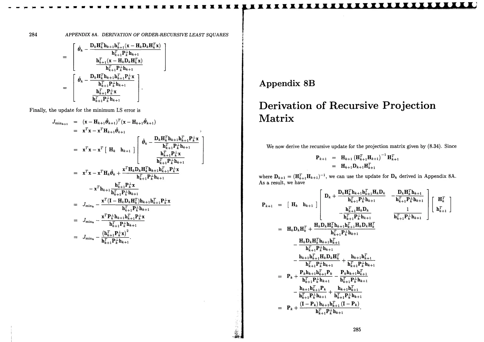
![__ ~~ __________ ~~~ ___ ••••••••• ••••••• IIIIIIIIIIIIIII.IIIA.J
Appendix Be
Derivation of Sequential Least Squares
In this appendix we derive (8.46)-(8.48).
8[n] (HT[n]C-1
[n]H[n]) -I HT[n]C-1
[n]x[n]
(
[ HT[n _ 1] h[n] 1[ C[n:; 1] O
2]-I [H[n - 1] ])-1
o an hT[n]
. ([ HT[n-l] h[n] 1[C[n:;l] O
2]-1 [x[n-l]]).
o an x[n]
Since the covariance matrix is diagonal, it is easily inverted to yield
Let
~[n - 1] = (HT[n - I]C-1[n - I]H[n _ 1])-1
which is the covariance matrix of e[n - 1]. Then,
286
APPENDIX 8e. DERIVATION OF SEQUENTIAL LEAST SQUARES 287
The first term in parentheses is just ~[n]. We can use Woodbury's identity (see
Appendix 1) to obtain
~[n] (
1 )-1
~-I[n - 1] + a~ h[n]hT[n]
~[n - 1] _ _
~"-[n_-_l-,-=]h:7-[n-7-]h--:T...:....[n...:....]~--,[n:-:---:--,-I]
a~ +hT[n]~[n - l]h[n]
(I - K[n]hT[n]) ~[n - 1]
where
K[n]- ~[n -1]h[n]
- a~ +hT[n]~[n - l]h[n]
Applying these results to e[n] yields
since
e[n] = (I - K[n]hT[n]) ~[n - 1]
. ( ~-I[n - l]e[n - 1] + :~h[n]x[n])
e[n - 1] = (HT[n - I]C-1
[n -1]H[n -1]) -I HT[n -1]C-1
[n - l]x[n - 1]
= ~[n - I]HT
[n -1]C-I
[n - l]x[n - 1].
Continuing, we have
But
e[n] = e[n - 1] + ~~[n - l]h[n]x[n]- K[n]hT[n]8[n - 1]
a~
1
- -K[n]hT[n]~[n -1]h[n]x[n].
172
n
and therefore
e[n] e[n -1] +K[n]x[n]- K[n]hT[n]e[n -1]
e[n - 1] +K[n] (x[n]- hT[n]e[n -1]) .](https://image.slidesharecdn.com/fundamentalsofstatisticalsignalprocessing-estimationtheory-kay-230513154707-1f7652e0/75/Fundamentals-Of-Statistical-Signal-Processing-Estimation-Theory-Kay-pdf-149-2048.jpg)
![288 APPENDIX Be. DERIVATION OF SEQUENTIAL LEAST SQUARES
Finally, to update the minimum LS error we have
(x[n] - H[n]8[n]) TC-1
[n] (x[n] - H[n]8[n])
xT[n]C-1[n] (x[n]- H[n]8[n])
[
C-l[n - 1] 0] [x[n - 1]- H[n - 1]8[n]]
[xT[n-1] x[n]l OT ~
a2 x[n] - hT[n]8[n]
n
xT[n -1]C-1
[n -1] (x[n -1]- H[n -1]8[n])
+ :2x[n] (x[n] - hT[n]8[n]) .
n
Let ern] = x[n]- hT[n]8[n - 1]. Using the update for 8[n] produces
)
Jrnin[n] xT[n - 1]C-1
[n - 1] (x[n - 1]- H[n - 1]8[n - 1]- H[n - l]K[n]e[n])
But
so that
and also
+ a~ x[n] (x[n] - hT[n]8[n - 1] - hT[n]K[n]e[n])
n
Jrnin[n - 1]- xT[n - 1]C-1
[n - l]H[n - l]K[n]e[n]
+ ~x[n] (1 - hT[n]K[nJ) ern].
a;
Jrnin[n] = Jrnin[n - 1]- 8T[n -1]:E-1
[n - l]K[n]e[n]
+ ~x[n] (1 - hT[n]K[nJ) ern]
a;
~x[n] (1 - hT[n]K[nJ) - 8T[n -1]:E-1
[n -l]K[n]
a;
1 ( hT[n]:E[n - l]h[n]) 8T[n - l]h[n]
a;x[n] 1 - a; +hT[n]:E[n - l]h[n] - a; + hT[n]:E[n - l]h[n]
x[n] - hT[n]8[n - 1]
a; +hT[n]:E[n - l]h[n]
ern]
a; + hT[n]:E[n - l]h[n]'
Hence, we have finally
e2
[n]
Jrnm[n] = Jrnin[n - 1] + a; +hT[n]:E [n - l]h[n]
Chapter 9
Method of Moments
9.1 Introduction
The approach known as the method 0/ moments is described in this chapter. It produces
an estimator that is easy to determine and simple to implement. Although the estimator
has no optimality properties it is useful if the data record is Ion enou h. This is
ecause the method of moments estimator is usually consistent. If the performance
is not satisfactory, then it can be used as an initial estimate, which is subsequently
improved through a Newton-Raphson implementation of the MLE. After obtaining the
method of moments estimator, we describe some approximate approaches for analyzing
its statistical performance. The techniques are general enough to be used to evaluate
the performance of many other estimators and are therefore useful in their own right.
9.2 Summary
The method of moments approach to estimation is illustrated in Section 9.3 with some
examples. In general, the estimator is iven b 9.11 for a vector arameter. The
Eerformance of the met 0 0 moments estimator may be partially characterized~
the approximate mean of (9.15) and the approximate variance of (9.16). Also,!!:!!l'
estimator that depends on a group of statistics whose PDF is concentrated about its
mean can make use of the same expressions. Another case where an approximate mea;
and variance evaluation is useful involves signal in noise problems when the SNR ~
high. Then, the estimation performance can be partially described by the approximate
mean of (9.18) and the approximate variance of (9.19).
9.3 Method of Moments'
The method of moments approach to estimation is based on the solution of a theoretical
equation involving the moments of a PDF. As an example, assume we observe x[n] for
n = 0,1, ... ,N - 1, which are liD samptes from the Gaussian mixture PDF (see also
289](https://image.slidesharecdn.com/fundamentalsofstatisticalsignalprocessing-estimationtheory-kay-230513154707-1f7652e0/75/Fundamentals-Of-Statistical-Signal-Processing-Estimation-Theory-Kay-pdf-150-2048.jpg)
![• • • • • • • • • • • • • • • • • • • • • • • • • • • •
290 CHAPTER 9. METHOD OF MOMENTS
Problem 6.14)
p(x[n]; f) = ~ exp (_~ x
2
[n]) + _f_ exp (_~ X2[~])
v27rar 2 ar V27ra? 2 a2
or in more succinct form
where
(,b;(x[n]) = _1_ exp (_~ X2[~]) .
v27rar 2 ai
The parameter f is termed the mixture parameter, which satisfies 0 < f < 1, and ai, a~
are the variances of the individual Gaussian PDFs. The Gaussian mixture PDF may
be thought of as the PDF of a random variable obtained from a N(O, ail PDF with
probability 1- f and from a N(o, an PDF with probability f. Now if ar, ai are known
and f is to be estimated, all our usual MVU estimation methods will fail. The MLE
will require the maximization of a very nonlinear function of f. Although this can
be implemented using a grid search, the method of moments provides a much simpler
estimator. Note that
E(x2[n]) = I:x2[n] [(1- f)cPl(x[n]) + fcP2(x[n])] dx[n]
= (l-f)a~+fa~ (9.1)
since the mean of x[n] is zero. This theoretical equation relates the unknown param-
eter f to the second moment. If we now replace E(x2
[n]) by its natural estimator
1 "N-l 2[ ] h
Iii L.m=O X n, we ave
1 N-l
N L x2
[n] = (1 - f)ai + fa~
n=O
(9.2)
and solving for f, we have our method of moments estimator
1 N-l
N Lx2[n]-a~
i. = n=O
a? - ar
(9.3)
The ease with which the estimator was found is due to the linear nature of the theoretical
moment equation (9.1). The estimator is easily shown to be unbiased (although this is
not generally the case). The variance of i. is found as
-.....-..._ ••• IIIIII .. IIIIIII .. IIIIIIIIIJ
9.3. METHOD OF MOMENTS
But it is easily shown that
E(x4
[n]) = (1 - f)3at + f3a~
which when combined with (9.1) produces the variance
(
0) _ 3(1- flat + 3fai - [(1 - f)ai + fai]2
var f - N( 2 _ 2)2
a2 a 1
291
(9.4)
To determine the loss in performance we could evaluate the CRLB (we would need to do
this numerically) and compare it to (9.4). If the increase in variance were substantial,
we could attempt to implement the MLE, which would attain the bound for large data
records. It should be observed that the method of moments estimator is consistent in
that i. -+ f as N -+ 00. This is because as N -+ 00, from (9.3) E(i.) = f and from (9.4)
var(i.) -+ O. Since the estimates of the moments that are substituted into the theoretical
equation approach the true moments for large data records, the equation to be solved
approaches the theoretical equation. As a result, the method of moments estimator
will in general be consistent (see Problem 7.5). In (9.2) for example, as N -+ 00, we
have
and the theoretical equation results. When solved for f, the true value is obtained.
We now summarize the method of moments for a scalar parameter. Assume that
the kth moment JJ.k = E(xk[n]) 'depends upon the unknown parameter () according to
JJ.k = h(8). (9.5)
We first solve for () as
() = h-1(JJ.k)
assuming h-1
exists. We then replace the theoretical moment by its natural estimator
1 N-l
{t.k = N L xk[riJ-
n=O
(9.6)
to yield the method of moments estimator
(9.7)
Some examples follow.
Example 9.1 - DC Level in WGN
If x[n] = A+w[n] is observed for n = 0,1, ... ,N -1, where w[n] is WGN with variance
a2
and A is to be estimated, then we know that
JJ.l = E(x[n]) = A.](https://image.slidesharecdn.com/fundamentalsofstatisticalsignalprocessing-estimationtheory-kay-230513154707-1f7652e0/75/Fundamentals-Of-Statistical-Signal-Processing-Estimation-Theory-Kay-pdf-151-2048.jpg)
![II . . . . . . ..
296 CHAPTER 9. METHOD OF MOMENTS
where the x[nl's are lID and each has an exponential distribution. To find the approx-
imate mean and variance we use (9.15) and (9.16). In this case we have
where
and
The mean of T1 is
1 N-1
T1 = N L x[n]
n=O
/11 = E(Td
1 N-1
N L E(x[n])
n=O
E(x[n])
1
A
using the results of Example 9.2. The variance of T1 is
But
var(x[n])
so that
(
1 N-1 )
var(Td = var N ~ x[n]
var(x[n])
N
1
00 1
x2
[n]A exp(-Ax[n]) dx[n]- -
o A2
2 1 1
1
var(Td = NA2 '
~I -_..!..-_A2
OT1T.=!". - /1~ - .
From (9.15) we have the approximate mean
9.5. STATISTICAL EVALUATION OF ESTIMATORS
and from (9.16) the approximate variance is
var(~) = :1IT.=!". var(T1
)::1IT.=!".
(_A2) N~2 (_A2)
A2
N
297
The estimator is seen to be approximately unbiased and has an approximate variance
decreasing with N. It should be emphasized that these expressions are only approxi-
mate. They are only as accurate as is the linearization of g. In fact, for this problem
~ can be easily shown to be the MLE. As such, its asymptotic PDF (as N -+ 00) can
be shown to be (see (7.8))
Hence, the approximation is accurate only as N -+ 00. (In Problem 9.10 quadratic
expansions of 9 are employed to derive the second-order approximations to the mean
and variance of i) To determine how large N must be for the mean and variance
expressions to hold requires a Monte Carlo computer simulation. <>
The basic premise behind the Taylor series approach is that the function 9 be approx-
imately linear over the range of T for which p(T; 8) is essentially nonzero. This occurs
naturally when
1. The data record is large so that p(T; 8) is concentrated about its mean, as in the pre-
vious example. There the PDF of T1 = it L~:01 x[n] becomes more concentrated
about E(T1 ) as N -+ 00 since var(T1 ) = 1/(NA2
) -+ 0 as N -+ 00.
2. The problem is to estimate the parameter of a signal in noise, and the SNR is
high. In this case, by expanding the function about the signal we can obtain the
approximate mean and variance. For a high SNR the results will be quite accurate.
This is because at a high SNR the noise causes only a slight perturbation of the
estimator value obtained in the case of no noise. We now develop this second case.
We consider the data
x[n] = s[n; 8] + w[n] n = 0, 1, ... ,N - 1
where w[n] is zero mean noise with covariance matrix C. A general estimator of the
scalar parameter 8 is
g(x)
g(8(8) +w)
h(w).](https://image.slidesharecdn.com/fundamentalsofstatisticalsignalprocessing-estimationtheory-kay-230513154707-1f7652e0/75/Fundamentals-Of-Statistical-Signal-Processing-Estimation-Theory-Kay-pdf-154-2048.jpg)
![~~ ..........................
298 CHAPTER 9. METHOD OF MOMENTS
In this case we may choose the statistic T as the original data since as the SNR becomes
larger, the PDF of T = x becomes more concentrated about its mean, which is the
signal. We now use a first-order Taylor expansion of 9 about the mean of x, which is
,." = s(0), or, equivalently, of h about w = O. This results in
8;::, h(O) + £ ~I w[n].
n=O ow[n] w=o
As before, it follows that approximately
E(8)
var(B)
h(O) = g(s(O))
oh IT C oh I
Ow w=o Ow w=o .
(9.17)
(9.18)
(9.19)
In most cases if there is no noise, the estimator yields the true value since g(s(0)) = O.
Hence, for a high SNR it will be unbiased. An example follows.
Example 9.5 - Exponential Signal in White Noise
For the data
x[n] = rn + w[n] n = 0, 1,2
where w[n] is zero mean uncorrelated noise with variance 0'2, the damping factor r is
to be estimated. Wishing to avoid a maximization of the likelihood to find the MLE
(see Example 7.11), we propose the estimator
, x[2] + x[l]
r= .
x[l] +x[O]
In terms of the signal and noise we have
and according to (9.18)
, _r2_+~w~[2:,--]+_r_+_w....;.[....;..I]
r = h(w) = r + w[l] + 1 + w[O]
r2 +r
E(f) = h(O) = r + 1 = r
or the estimator is approximately unbiased. To find the variance
oh I r2 + w[2] + r + w[l] I
ow[0] w=o = - (r + w[l] + 1 + W[0])2 w=o
r2 +r
(r + 1)2
r
r+l
••••••••• IIIIIIIIIIIIIIIII.Il
9.6. SIGNAL PROCESSING EXAMPLE
Similarly,
oh I
ow[l] ..=0
oh I
ow[2] w=o
r-l
r+l
1
r+l
Since C = 0'21, we have from (9.19)
2 ( oh I )2
var(f) = 0'2 L --
n=O ow[n] w=o
0'2 2 2
(r + 1)2 [r + (r - 1) + 1]
2
2r2 - r + 1
0' •
(r + 1)2
299
<)
It is also worthwhile to remark that from (9.14) and (9.17) the estimators are approx-
imately linear functions of T and w, respectively. If these are Gaussian, then 8 will
also be Gaussian - at least to within the approximation assumed by the Taylor expan-
sion. Finally, we should note that for a vector parameter the approximate mean and
variance for each compont;.nt can be obtained by applying these techniques. Obtaining
the covariance matrix of (J is possible using a first-order Taylor expansion but can be
extremely tedious.
9.6 Signal Processing Example
We now apply the method of moments and the approximate performance analysis to
the problem of frequency estimation. Assume that we observe
x[n] = Acos(211'fon + </J) + w[n] n = 0,1, ... ,N - 1
where w[n] is zero mean white noise with variance 0'2. The frequency fa is to be
estimated. This problem was discussed in Example 7.16 in which the MLE of frequency
was shown to be approximately given by the peak location of a periodogram. In an
effort to reduce the computation involved in searching for the peak location, we now
describe a method of moments estimator. To do so we depart slightly from the usual
sinusoidal model to assume that the phase </J is a random variable independent of w[n]
and distributed as </J rv UfO, 211']. With this assumption the signal s[n] = A cos(211'fan +
</J) can be viewed as the realization of a WSS random process. That this is the case is
verified by determining the mean and ACF of s[n]. The mean is](https://image.slidesharecdn.com/fundamentalsofstatisticalsignalprocessing-estimationtheory-kay-230513154707-1f7652e0/75/Fundamentals-Of-Statistical-Signal-Processing-Estimation-Theory-Kay-pdf-155-2048.jpg)
![·-~~ ..---~.-~~~~-~--.- ..-...
300 CHAPTER 9. METHOD OF MOMENTS
and the ACF is
E(s[n]) E[A COS(27Tfon +4»)
r2~ 1
io A COS(27Tfon + 4» 27T d4>
o
E[s[n)s[n + k))
E[A2 cos(27Tfon + 4» cos(27Tfo(n + k) + 4»)
A2E [~COS(47Tfon + 27Tfok + 24» + ~ cos 27Tfok]
A2
- cos 27Tfok.
2
The ACF of the observed process becomes
To simplify the discussion and the subsequent estimator we will assume that the signal
amplitude is known (see Problem 9.12 for the unknown amplitude case). We will let
A = yI2, so that the ACF becomes
Txx[kj = cos 27Tfok +0'26[k).
To estimate the frequency by the method of moments approach we observe that
rxx[l) = cos2rrfo,
and therefore without having to assume knowledge of 0'2 we can implement the method
of moments estimator
. 1
fo = - arccos Txx[l)
27T
where Txx[l) is an estimator of Txx[l). A reasonable estimator of the ACF for k = 1 is
1 N-2
Txx[l) = N _ 1 L x[n)x[n + 1)
n=O
so that finally we have for our frequency estimator
1 [1 N-2 ]
io = - arccos -N L x[n)x[n + 1) .
27T - 1 n=O
(9.20)
• • • • • • • • • • • • • • • • • • • • • • • • • • • • • 1
9.6. SIGNAL PROCESSING EXAMPLE 301
The argument of the arccos function may exceed 1 in magnitude, usually occurring
when the SNR is low. If this is the case, the estimate is meaningless and it is indicative
of an unreliable estimator.
Although motivated by the random phase sinusoidal model, this estimator remains
valid if 4> is dete:ministic and unknown (see Problem 9.11). In determining the mean
and variance of fo we assume that 4> is deterministic. To assess the performance of our
estimator we use the first-order Taylor expansion approach and expand about the point
w = O. Thus, the obtained performance is valid for high enough SNR. From (9.18) we
have
1 [1 N-2 ]
E(jo) 27T arccos N -1 ~ ..;2cos(27Tfon + 4»..;2cos(27Tfo(n + 1) + 4»
1 [1 N-2 ]
= 27T arccos N _ 1 ~ (cos(47Tfon + 27Tfo + 24» +cos 27Tfo) .
The double-frequency term when summed is approximately zero, so that at a high SNR
1
27T arccos [cos 27Tfo)
fo· (9.21)
To find the variance we note that
so that the first-order partials are
oh I 1 1 ou I
ow[i) w=o = - 27T Jf="U2 ow[i) w=o'
But
ou I IoN-2 I
ow[i) w=o = N - 1 ow[i) ~(s[n)w[n + 1) + w[n)s[n + 1]) ...=0
with the other terms in the sum resulting in zero after differentiating and letting w = O.
Continuing, we have
{
N~IS[l) i = 0
ou I 1 ( [. .
ow[i) ...=0 = N-I S t - 1) + s[t + 1]) i = 1,2, ... , N - 2
N~l s[N - 2) i = N - 1](https://image.slidesharecdn.com/fundamentalsofstatisticalsignalprocessing-estimationtheory-kay-230513154707-1f7652e0/75/Fundamentals-Of-Statistical-Signal-Processing-Estimation-Theory-Kay-pdf-156-2048.jpg)
![302 CHAPTER 9. METHOD OF MOMENTS
Also,
1 N-2
N -1 L s[n)s[n+ 1]
n=O
"'" cos 27rfo
as already shown. Thus,
ah I
aw[i) w=o
au I
27rsin27rfo aw[i) w=o'
1
From (9.19) with C = 0"21 we obtain
N-l( ah I )2
var(jo) = 0"2 L --
n=O aw[n) w=o
But s[n - 1) + s[n + 1) = 2cos27rfos[n), as can easily be verified, so that finally the
variance of the frequency estimator is for a high SNR
(9.22)
where s[n) = v'2cos(27rfon + ¢). The evaluation of the variance is straightforward,
although tedious. Note that the variance decreases most rapidly as 1/N2 (for fo = 1/4)
versus the 1/N3
dependence for the CRLB (see (3.41)). Additionally, for fo near 0 or
1/2 the variance increases rapidly. This is due to the arccos operation required to
determine fa. As shown in Figure 9.1, a slight perturbation in the argument for x near
±1 (fo near 0 or 1/2) will cause large fluctuations in the function value due to the steep
slope.
As an example of the accuracy of the approximate mean and variance expressions,
we consider the data set with parameters SNR = A2/20"2 = 1/0"2 for A = v'2 and
fa = 0.2, ¢ = 0, and N = 50. For w[n) being WGN a Monte Carlo computer simulation
in which 1000 realizations of fo as given by (9.20) were generated for each of several
SNRs. In Figure 9.2a the actual mean E(jo) obtained, as well as the theoretical mean
of fo = 0.2, are shown versus SNR. As expected for a high enough SNR, the estimator
is essentially unbiased. The slight discrepancy is due to the approximations made in
deriving the estimator, principally that N was large enough to neglect the double-
frequency term. For larger N it can be verified that the mean equals the true value
9.6. SIGNAL PROCESSING EXAMPLE
303
arccos(x)
1 :
fo = - ,
2 "': /'
-1
fo = 0
Figure 9.1 Explanation for in-
x = cos 27Tfo creased variance of frequency esti-
mator
0.220
0.215
0.210
<=
oj
0.205
Il)
::;s
0.200
0.195
-10
-20-+
Il) !
~ -25-+
I
-5
.~ -301-·····....
~ -35J ......
o "
.,;; -40-+
.£ ,
~ -45-f
-50j'
-55
/ActUaI
..............................., ~~~:~:i~~;.
I
o 5
SNR (dB)
(a)
10 15
I
20
~0~1-------,1-------,1------~1-------,1______-T1_______1
-10 -5 0 5 10 15 20
SNR (dB)
(b)
Figure 9.2 Method of moments frequency estimator](https://image.slidesharecdn.com/fundamentalsofstatisticalsignalprocessing-estimationtheory-kay-230513154707-1f7652e0/75/Fundamentals-Of-Statistical-Signal-Processing-Estimation-Theory-Kay-pdf-157-2048.jpg)
![304 CHAPTER 9. METHOD OF MOMENTS
for a high SNR. Correspondingly, in Figure 9.2b the actual variance obtained and
the theoretical variance as determined from (9.22) are shown versus SNR. The same
behavior is evident. Some further discussions of this example can be found in Problem
9.13. For further discussions of this estimation approach the reader should consult
[Lank et al. 1973, Kay 1989].
References
Kay, S., "A Fast and Accurate Single Frequency Estimator," IEEE Trans. Acoust., Speech, Signal
Process., Vo!' 37, pp. 1987-1990, Dec. 1989.
Lank, G.W., 1.8. Reed, G.E. Pollon, "A Semicoherent Detection and Doppler Estimation Statistic,"
IEEE Trans. Aerosp. Electron. Systems, Vo!' 9, pp. 151-165, March 1973.
Rider, P.R., "Estimating the Parameters of Mixed Poisson, Binomial, and Weibull Distributions
by the Method of Moments," Bull. Int. Statist. Inst., Vo!' 38, pp. 1-8, 1961.
Problems
9.1 If N lID observations {x [0], x[l], ... ,x[N - In are made from the Rayleigh PDF
find a method of moments estimator for (J2.
x>O
x<O
9.2 If N lID observations {x[O], x[l]' ... ,x[N - In are made from the Laplacian PDF
1 (v'2lxl)
p(x; (J) = -- exp - - -
"fi(J (J
find a method of moments estimator for (J.
9.3 Assume that N lID samples from a bivariate Gaussian PDF are observed or
{xQ' Xl.' .. xN-d, where each x is a 2 x 1 random vector with PDF x,....., N(O, C).
If
C=[~ i]
find a method of moments estimator for p. Also, determine a cubic equation to be
solved for the MLE of p. Comment on the ease of implementation of the different
estimators.
9.4 If N lID observations {x[O],x[l], ... ,x[N - In are made from the N(J.L,(J2) PDF,
find a method of moments estimator for () = [J.L a2JT.
.......... IIIIIIIIIIIIIIJ;IIIIII)
PROBLEMS
305
9.5 In Example 8.12 we determined that the ACF of an ARMA process satisfies the
recursive difference equation
p
rxx[n] = - L a[k]rxx[n - k] n>q
k=]
where {a[l], a[2], ... ,alP]} denote the AR filter parameters and q is the MA order.
Propose a method of moments estimator for the AR filter parameters.
9.6 For a DC level in WGN or
x[n] = A +w[n] n = O,l, ... ,N - 1
where w[n] is WGN with variance a2
, the parameter A2 is to be estimated. It is
proposed to use
A2 = (xj2.
For this estimator find the approximate mean and variance using a first-order
Taylor expansion approach.
9.7 For the observed data
x[n] = cos¢> +w[n] n = 0, 1, ... , N - 1
where w[n] is WGN with variance a2
, find a method of moments estimator for
¢>. Assuming the SNR is high, determine the approximate mean and variance for
your estimator using the first-order Taylor expansion approach.
9.8 In this problem we determine the mean of an estimator to second order by using a
second-order Taylor expansion. To do so expand (j = g(T) about the mean of T
or T = J.L, retaining the terms up to and including the quadratic term. Show that
the approximate mean of (j is
where
Hint: Use the result
9.9 In this problem we determine the approximate variance of an estimator to second
~rder or by using a second-order Taylor expansion approach. To do so first expand
() = g(T) about the mean of T or T = J.L, retaining the terms up to and including](https://image.slidesharecdn.com/fundamentalsofstatisticalsignalprocessing-estimationtheory-kay-230513154707-1f7652e0/75/Fundamentals-Of-Statistical-Signal-Processing-Estimation-Theory-Kay-pdf-158-2048.jpg)
![306
-------.,....,..,~ ............ --
CHAPTER 9. METHOD OF MOMENTS
the quadratic term. Next, use the results of Problem 9.8 and finally make the
assumption that T ~ N(J-L, CT ). You should be able to verify the following result:
, og IT og I 1
var(O) = -;:;- CT "'T + -2tr [(G(J-L)CT)2].
uT T=J-L u T=J-L
The r x r G(J-L) is defined in Problem 9.8. Hint: You will need the following result,
which is valid for a symmetric N x N matrix A,
9.10 Using the results of Problems 9.8 and 9.9 find the approximate mean and variance
to second order for the estimator of .A discussed in Example 9.4. Ho'f do your
results compare to the first-order result? Be sure to justify the approximate
Gaussian PDF of x, required to apply the variance expression. Also, compare the
results to those predicted from asymptotic MLE theory (recall that the estimator
is also the MLE).
9.11 Prove that for a sinusoidal signal
s[n] = A cos(21l-Jon + ¢)
where the phase ¢ is deterministic but unknown, that
1 N-2 A2
N _ 1 L s[n]s[n + 1]-+ 2 cos 27rfo
n=O
as N -+ 00. Assume that fa is not near 0 or 1/2. Hence, comment on the use of
the method of moments estimator proposed in the signal processing example in
Section 9.6 for the deterministic phase sinusoid.
9.12 To extend the applicability of the frequency estimator proposed in the signal
processing example in Section 9.6 now assume that the signal amplitude A is
unknown. Why can't the proposed estimator (9.20) be used in this case? Consider
the estimator
, 1 [N~l~x[n]x[n+l]
fa = - arccos N 1 •
27r 1 -
N L x
2
[n]
n=O
Show that at a high SNR and for large N, E(jo) = fa. Justify this estimator
as a method of moments estimator based on the ACF. Would you expect this
estimator to work well at a lower SNR?
.--_ • • • • • • • • • I I I I • • • • • • • • • • • J
PROBLEMS
307
9.13 For the signal processing example in Section 9.6 assume that the parameters are
A = .J2, fa = 0.25, ¢ = 0, and that N is odd. Show that from (9.22) var(jo) = O.
To understand this result note that
oh I
ow[iJ ...=0 = 0
for i = 0, 1, ... , N -1. What does this say about the first-order Taylor expansion
approximation? How could you improve this situation?](https://image.slidesharecdn.com/fundamentalsofstatisticalsignalprocessing-estimationtheory-kay-230513154707-1f7652e0/75/Fundamentals-Of-Statistical-Signal-Processing-Estimation-Theory-Kay-pdf-159-2048.jpg)
![310
CHAPTER 10. THE BAYESIAN PHILOSOPHY
P.4(~; A)
-Ao
(a) PDF of sample mean
(b) PDF of truncated sample mean
Figure 10.1 Improvement of estimator via prior knowledge
1" ate the realization of a random variable based on data is described in Section ~0.5
: ~~ing due to th~ ~orrelation ?etw;~~th~e~~~:o:;~;:~~:~,p~~~~:~i~O~S~u:;::~::~~
the result that a Jomtly Gaussian. y (1025) This is then applied to the)Bayesian
h . (1024) and a covariance . . A
avmg a mean· . t ·or PDF as summarized in Theorem 10.3. s
linear model of (10.26) to Yield the pos erl
f
h t' PDF (10 28) is the minimum
. h . eha ter 11 the mean 0 t e pos erlor .
wIll be s. own m p , ter Section 10.7 discusses nuisance parameters from
11SE eS~lmat~r for .a vectho:IPaSramt'~n io 8 describes the potential difficulties of using a
a Bayesian vlewpomt, w Ie. ec I . '.
Bayesian estimator in a classical estimatIOn problem.
10.3 Prior Knowledge and Estimation
It is a fundamental :uletof eS;~~:~:;fee~?at:::a~:t~~ei:~~~~~~~~~;~~dIT: :il~l~~~:~
~ more accurate estl:~~~timator should produce only estimates within that interva!.
mterval, then an~ g h that the MVU estimator of A is the sample mean x.
In Example 3.1 It was sown" . I A <
However, this assumed :hat .A could take on anyo~:~~: : ~:~::~at-;c~ take ~~
Due to physical constramts It may be more AreasT t' A" _ - as the best estimator
. fi"t I A <A< oream-x
~~~I~a~~e~~~:~;at7~t:i~:eeTm~y ;icld v~lue~·outside the known interva~. As shown
in Figure 10.la, this is due to noise effects. eertainl~, we would expect to Improve our
estimation if we used the truncated sample mean estimator
. {-Ao
A= i
Ao
i < -Au
-Ao ~ i ~ Ao
i > Ao
which would be consistent with the known constraints. Such an estimator would have
the PDF
Pr{i ~ -Ao}8(~ + Ao)
+PA (~; A)[u(~ + Ao) - u(~ - Ao)]
+ Pr{i :::: Ao}8(~ - Ao) (10.1)
10.3. PRIOR KNOWLEDGE AND ESTIMATION 311
where u(x) is the unit step function. This is shown in Figure 1O.lb. It is seen that A
is a biased estimator. However, if we compare the MSE of the two estimators, we note
that for any A in the interval - Ao ~ A ~ Ao
mse(..1) = 1:(~ -Aj2pA(~; A) d~
1:°(~ -A)2pA(~; A) d~ +1::(~ -A)2pA(~; A) d~
+ r (~- A)2pA(~;A)~
lAo
> 1:°(-Ao - A)2pA(~; A) d~ +1:°0(~- A)2pA(~;A) ~
+ roo(Ao-A)2pA(~;A)d~
lAo
mse(A).
Hence, A, the truncated sample mean estimator, is better than the sample mean esti-
mator in terms of MSE. Although Ais still the MVU estimator, we have been able to
reduce the mean square error by allowing the estimator to be biased. In as much as
we have been able to produce a better estimator, the question arises as to whether an
optimal estimator exists for this problem. (The reader may recall that in the classical
case the MSE criterion of optimality usually led to unrealizable estimators. We shall
see that this is not a problem in the Bayesian approach.) We can answer affirmatively
but only after reformulating the data model. Knowing that A must lie in a known
interval, we suppose that the true value of A has been chosen from that interval. We
then model the process of choosing a value as a random event to which a PDF can
be assigned. With knowledge only of the interval and no inclination as to whether A
should be nearer any particular value, it makes sense to assign a U[-Ao, Ao] PDF to
the random variable A. The overall data model then appears as in Figure 10.2. As
shown there, the act of choosing A according to the given PDF represents the departure
of the Bayesian approach from the classical approach. The problem, as always, is to
estimate the value of A or the realization of the random variable. However, now we
can incorporate our knowledge of how A was chosen. For example, we might attempt
to find an estimator Athat would minimize the Bayesian MSE defined as
Bmse(..1) = E[(A - ..1)2]. (10.2)
We choose to define the error as A - Ain contrast to the classical estimation error of
A- A. This definition will be useful later when we discuss a vector space interpretation
of the Bayesian estimator. In (10.2) we emphasize that since A is a random variable, the
expectation operator is with respect to the joint PDF p(x, A). This is a fundamentally
different MSE than in the classical case. We distinguish it by using the Bmse notation.
To appreciate the difference compare the classical MSE
mse(..1) = J(A - A)2p(X; A) dx (10.3)](https://image.slidesharecdn.com/fundamentalsofstatisticalsignalprocessing-estimationtheory-kay-230513154707-1f7652e0/75/Fundamentals-Of-Statistical-Signal-Processing-Estimation-Theory-Kay-pdf-161-2048.jpg)
![312
CHAPTER 10. THE BAYESIAN PHILOSOPHY
PDF 1
~:o
x[n] n = 0, 1. ... , IV - 1
, ,
, _____________________ 1
Bayesian philosophy
Figure 10.2 Bayesian approach to data modeling
to the Bayesian MSE
Bmse(A) = j j (A - A)2p(X, A) dxdA. (10.4)
Even the underlying experiments are different, as is reflected in the averaging PDFs.
If we were to assess the MSE performance using a Monte Carlo computer simulation,
then for the classical approach we would choose a realization of w[n] and add it to a
given A. This procedure would be repeated M times. Each time we would ~dd.a new
realization of w[n] to the same A. In the Bayesian approach, for each realIzatIOn we
would choose A according to its PDF U[-Ao, Ao] and then generate w[n] (assuming
that w[n] is independent of A). We would then repeat this procedure M t.im~s. In
the classical case we would obtain a MSE for each assumed value of A, while III the
Bayesian case the single MSE figure obtained would be an average over.the PDF of
A. Note that whereas the classical MSE will depend on A, and hence estimators that
attempt to minimize the MSE will usually depend on A (see Section 2.4), the Bayesian
MSE will not. In effect, we have integrated the parameter dependence away! It should
be clear that comparing classical and Bayesian estimators is like comparing "apples
and oranges." The reader who is tempted to do so may become thoroughly confused.
Nonetheless, at times, the forms of the estimators will be identical (see Problem 10.1).
To complete our example we now derive the estimator that minimizes the Bayesian
MSE. First, we use Bayes' theorem to write
p(x, A) = p(Alx)p(x)
so that
Bmse(A) = j [j(A - A)2p(Alx) dA) p(x) dx.
Now since p(x) 2 0 for all x, if the integral in brackets can be mi,nimized for each x,
then the Bayesian MSE will be minimized. Hence, fixing x so that A is a scalar variable
10.3. PRIOR KNOWLEDGE AND ESTIMATION
-Ao
ptA)
1
2Ao
A
Ao
p(Alx)
-Ao X Ao
E(Alx)
(a) Prior PDF (b) Posterior PDF
Figure 10.3 Comparison of prior and posterior PDFs
(as opposed to a general function of x), we have
~ j(A - A)2p(Alx) dA =
8A
-,(A - A)2p(Alx) dA
j 8 '
8A
j -2(A - A)p(Alx) dA
-2 j Ap(Alx) dA + 2A j p(Alx) dA
which when set equal to zero results in
A = j Ap(Alx) dA
or finally
A = E(Alx)
313
A
(10.5)
since the conditional PDF must integrate to 1. It is seen that the optimal estimator in
terms of minimizing the Bayesian MSE is the mean of the posterior PDF p(Alx) (see
also Problem 10.5 for an alternative derivation). The posterior PDF refers to the PDF
of A after the data have been observed. In contrast, peA) or
peA) = j p(x, A) dx
may be thought of as the prior PDF of A, indicating the PDF before the data are
observed. We will henceforth term the estimator that minimizes the Bayesian MSE
the minimum mean square error (MMSE) estimator. Intuitively, the effect of observing
data will be to concentrate the PDF of A as shown in Figure 10.3 (see also Problem
10.15). This is because knowledge of the data should reduce our uncertainty about A.
We will return to this idea later.](https://image.slidesharecdn.com/fundamentalsofstatisticalsignalprocessing-estimationtheory-kay-230513154707-1f7652e0/75/Fundamentals-Of-Statistical-Signal-Processing-Estimation-Theory-Kay-pdf-162-2048.jpg)
![- - - : - - ~ -- . .
314 CHAPTER 10. THE BAYESIAN PHILOSOPHY
In determining the MMSE estimator we first require the posterior PDF. We can use
Bayes' rule to determine it as
p(Alx)
p(xIA)p(A)
p(x)
p(xIA)p(A)
Jp(xIA)p(A) dA'
(10.6)
Note that the denominator is just a normalizing factor, independent of A, needed to
ensure that p(Alx) integrates to 1. If we continue our example, we recall that the prior
PDF p(A) is U[-Ao, AoJ. To specify the conditional PDF p(xIA) we need to further
assume that the choice of A via p(A) does not affect the PDF of the noise samples or
that w[nJ is independent of A. Then, for n = 0,1, ... , N - 1
and therefore
px(x[nllA) pw(x[nJ - AlA)
pw(x[nJ- A)
_1_ exp [__I_(x[nJ
- A)2]
..,j27r(J2 2(J2
[
1 N-J ]
p(xIA) = 1 N exp --2
2 L (x[nJ - A)2 .
(27r(J2) 2' (J n=O
(10.7)
It is apparent that the PDF is identical in form to the usual classical PDF p(x; A). In
the Bayesian case, however, the PDF is a conditional PDF, hence the "I" separator,
while in the classical case, it represents an unconditional PDF, albeit parameterized
by A, hence the separator ";" (see also Problem 10.6). Using (10.6) and (10.7), the
posterior PDF becomes
p(Alx) =
1 [1 N-J ]
2A
o
(27r(J2)'f exp --2(J-2 ~(x[nJ- A?
IAI :s Ao
J
AO 1 [1 N J ]
---2--"I:!.. exp --2
2 L (x[nJ - A)2 dA
-Ao 2Ao(27r(J ) 2 (J n=O
o IAI > Ao·
But
N-J N-J
L(x[nJ- A)2 L x2[nJ- 2NAx + NA2
n=O n=O
N-l
N(A - X)2 + L x2[nJ- Nx2
n=O
10.3. PRIOR KNOWLEDGE AND ESTIMATION 315
so that we have
--;:1=2 exp [--h-(A - X)2]
cV27r%:i 27'1
IAI :s Ao
(10.8)
o IAI >Ao
The factor c is determined by the requirement that p(Alx) integrate to 1, resulting in
JAO 1 [1 ]
c = - - - 2 exp -~(A - £)2 dA.
-Ao V 27r%:i 2N
The PDF is seen <0 be a truncated Gaussian, as shown in Figure 1O.3b. The MMSE
estimator, which is the mean of p(Alx), is
E(Alx)
1:Ap(Alx) dA
JAO 1 [1 ]
A---
2
exp -~(A - x? dA
-Ao V 27r%:i 2N
(10.9)
JAO 1 [1 ].
- - - 2 exp -~(A - X)2 dA
-Ao yi27r%:i 2N
Although this cannot be evaluated in closed form, we note that Awill be a function of
x as well as of Ao and (J2 (see Problem 10.7). The MMSE estimator will not be x due
to the truncation shown in Figure 1O.3b unless Ao is so large that there is effectively no
truncation. This will occur if Ao » J(J2/N. Otherwise, the estimator will be "biased"
towards zero as opposed to being equal to X. This is because the prior knowledge
embodied in p(A) would in the absence of the data x produce the MMSE estimator
(see Problem 10.8)
The effect of the data is to position the posterior mean between A = 0 and A = x in a
compromise between the prior knowledge and that contributed by the data. To further
appreciate this weighting consider what happens as N becomes large so that the data
knowledge becomes more important. As shown in Figure 10.4, as N increases, we have
from (10.8) that the posterior PDF becomes more concentrated about x (since (J2/N
decreases). Hence, it becomes nearly Gaussian, and its mean becomes just x. The
MMSE estimator relies less and less on the prior knowledge and more on the data. It
is said that the data "swamps out" the prior knowledge.](https://image.slidesharecdn.com/fundamentalsofstatisticalsignalprocessing-estimationtheory-kay-230513154707-1f7652e0/75/Fundamentals-Of-Statistical-Signal-Processing-Estimation-Theory-Kay-pdf-163-2048.jpg)
![- ~ ~ - - - - - - - - - - - - - - - - - - ~ - - - -
316 CHAPTER 10. THE BAYESIAN PHILOSOPHY
p(Alx) p(Alx)
A
~ Ao
-Ao
A
X"" E(Alx)
(a) Short data record (b) Large data record
Figure 10.4 Effect of increasing data record on posterior PDF
The results of this example are true in general and are now summarized. The
Bayesian approach to parameter estimation assumes that the parameter to be estimated
is a realization of the random variable B. As such, we assign a prior PDF p(B) to it. After
the data are observed, our state of knowledge about the parameter is summarized by
the posterior PDF p(Blx). An optimal estimator is defined to be the one that minimizes
the MSE when averaged over all realizations of () and x, the so-called Bayesian MSE.
This estimator is the mean of the posterior PDF or iJ = E(Blx). The estimator is
determined explicitly as
iJ = E(Blx) = JBp(Blx) dB. (10.10)
The MMSE estimator will in general depend on the prior knowledge as well as the
data. If the prior knowledge is weak relative to that of the data, then the estimator
will ignore the prior knowledge. Otherwise. the estimator will be "biased" towards the
prior mean. As expected, the use of prior information always improves the estimation
accuracy (see Example 10.1).
The choice of a prior PDF is critical in Bayesian estimation. The wrong choice will
result in a poor estimator, similar to the problems of a classical estimator designed with
an incorrect data model. Much of the controversy surrounding the use of Bayesian
estimators stems from the inability in practice to be able to justify the prior PDF.
Suffice it to say that unless the prior PDF can be based on the physical constraints of
the problem, then classical estimation is more appropriate.
10.4 Choosing a Prior PDF
As shown in the previous section, once a prior PDF has been chosen, the MMSE
estimator follows directly from (10.10). There is no question of existence as there is
with the MVU estimator in the classical approach. The only practical stumbling block
that remains, however, is whether or not E(Blx) can be determined in closed form. In
. - - - - - --- -. --. . . . .... -----. . -
10.4. CHOOSING A PRIOR PDF 317
the introductory example the posterior PDF p(Alx) as given by (10.8) could not be
found explicitly due to the need to normalize p(xIA)p(A) so that it integrates to 1.
Additionally, the posterior mean could not be found, as evidenced by (10.9). We would
have to resort to numerical integration to actually implement the MMSE estimator.
This problem is compounded considerably in the vector parameter case. There the
posterior PDF becomes
p(8Ix) = p(xI8)p(8)
Jp(xI8)p(8) d8
which requires a p-dimensional integration over 8. Additionally, the mean needs to
be evaluated (see Chapter 11), requiring further integration. For practical MMSE
estimators we need to be able to express them in closed form. The next example
illustrates an important case where this is possible.
Example 10.1 - DC Level in WGN - Gaussian Prior PDF
We now modify our prior knowledge for the introductory example. Instead of assuming
the uniform prior PDF
IAI ~ Ao
IAI > Ao
which led to an intractable integration, consider the Gaussian prior PDF
p(A) = _1_ exp [__l_(A - J-LA)2] .
J27ra~ 2a~
The two prior PDFs clearly express different prior knowledge about A, although with
J-LA = 0 and 3aA = Ao the Gaussian prior PDF could be thought of as incorporating
the knowledge that IAI ~ Ao. Of course, values of A near zero are thought to be more
probable with the Gaussian prior PDF. Now if
p(xIA)
1 [1 N-J ]
(27ra2)~ exp - 2a2 ?;(x[nJ- A)2
1 [1 N-J ] [ 1 ]
---lY.;:;- exp --2
2 L x2
[nJ exp --2 (NA2 - 2NAx)
(27ra2
) 2 a n=O 2a
we have](https://image.slidesharecdn.com/fundamentalsofstatisticalsignalprocessing-estimationtheory-kay-230513154707-1f7652e0/75/Fundamentals-Of-Statistical-Signal-Processing-Estimation-Theory-Kay-pdf-164-2048.jpg)
![~ ......... · · · · · .. · · · · -------i. --· -· · · .. ............I . _ • • a •.'
318
p(Alx)
CHAPTER 10. THE BAYESIAN PHILOSOPHY
p(xIA)p(A)
Jp(xIA)p(A) dA
1 [ 1 N-l ] [1 ]
N exp --2 L x2[n] exp --2 (NA2 - 2NAx)
(27l"(T2) T J27l"(T~ 2(T n-O 2(T
i:exp [-~ (:2(NA2 - 2NAx) + :~ (A - JjA)2)] dA
exp [-~Q(A)]
Note, however, that the denominator does not depend on A, being a normalizing factor,
and the argument of the exponential is quadratic in A. Hence, p(Alx) must be a
Gaussian PDF whose mean and variance depend on x. Continuing, we have for Q(A)
N 2 2NAx A2 2JjAA Jj~
-A ---+2---2-+2
(T2 (T2 (TA (TA (TA
Q(A) =
(
N +~) A2 _ 2 (N x +Jj:) A +Jj~ .
(T2 (T~ (T2 (TA (TA
Let
1
JjAlx =
Then, by completing the square we have
2 2
1 (2 2) JjAlx Jj.4
Q(A) = -2- A - 2JjAlxA + JjAlx - -2- + 2
(TAlx (TAlx (TA
10.4. CHOOSING A PRIOR PDF
so that
p(Alx)
1 2 2
)
2 JjAlx JjA
-2-(A - JjAlx - -2- + 2"
(TAlx (TAlx (TA
[ 1( )2] [1 (Jj~ Jj~IX)]
exp --2- A - JjAlx exp -- 2" - -2-
2(TAlx 2 (TA (TAlx
JOO [1 2] [1 (Jj~ Jj~IX)]
exp --2-(A - JjAlx) exp -- 2" - -2-
-00 2(TAlx 2 (TA (TAlx
--==l==exp [--;-(A - JjAlx)2]
r:;;;;;z- 2(TAIx
V~"u Alx
319
dA
where the last step follows from the requirement that p(Alx) integrate to 1. The pos-
terior PDF is also Gaussian, as claimed. (This result could also have been obtained by
using Theorem 10.2 since A, x are jointly Gaussian.) In this form the MMSE estimator
is readily found as
A E(Alx)
or finally, the MMSE estimator is
(10.11)
where
(T2
a = A 2.
(T~ + lv
Note that a is a weighting factor since 0 < a < 1. Using a Gaussian prior PDF, we
are able to determine the MMSE estimator explicitly. It is interesting to examine the
interplay between the prior knowledge and the data. When there is little data so that
(T~ «(T2IN, a is small and A~ JjA, but as more data are observed so that (T~ »(T2IN,
a ~ 1 and A~ x. The weighting factor a depends directly on our confidence in the prior
knowledge or (T~ and the data knowledge or (T2IN. (The quantity (T2IN is interpreted
as the conditional variance or E[(x - A)2IA]). Alternatively, we may view this process
by examining the posterior PDF as N increases. Referring to Figure 10.5, as the data
record length N increases, the posterior PDF becomes narrower. This is because the](https://image.slidesharecdn.com/fundamentalsofstatisticalsignalprocessing-estimationtheory-kay-230513154707-1f7652e0/75/Fundamentals-Of-Statistical-Signal-Processing-Estimation-Theory-Kay-pdf-165-2048.jpg)
![320
p(Alx)
posterior variance
CHAPTER 10. THE BAYESIAN PHILOSOPHY
"'p(A)
A
Figure 10.5 Effect of increasing
data record length on posterior PDF
2 1
var(Alx) = 17Alx = N 1 (10.12)
-+-
172
(j~
will decrease. Also, the posterior mean (10.11) or A will also change with increasing
N. For small N it will be approximately /-LA but will approach x for increasing N. In
fact, as N -+ 00, we will have A -+ x, which in turn approaches the true value of A
chosen. Observe that if there is no prior knowledge, which can be modeled by letting
(j~ -+ 00, then A-+ xfor any data record length. The "classical" estimator is obtained.
Finally, it was originally claimed that by using prior knowledge we could improve the
estimation accuracy. To see why this is so recall that
where we evaluate the expectation with respect to p(x, A). But
Bmse(A)
Since A= E(Alx), we have
Bmse(A)
JJ(A - A)2p(X, A) dxdA
JJ(A - A)2p(Alx) dAp(x) dx.
JJ[A - E(Alx)fp(Alx) dAp(x) dx
Jvar(Alx)p(x) dx. (10.13)
We see that the Bayesian MSE is just the variance 0/ the posterior PDF when averaged
over the PDF o/x. As such, we have
Bmse(A)
N 1
-+-
172
(j~
- ~ ~ - - - -- - -----~ -- -- )
10.5. PROPERTIES OF THE GAUSSIAN PDF
since (j~:x does not depend on x. This can be rewritten as
so that finally we see that
Bmse(A) = - A 2
172 ( 17
2
)
N 172
+ '!.-
A N
• 172
Bmse(A) < N
321
(10.14)
where 172
/ N is the minimum MSE obtained when no prior knowledge is available (let
(j~ -+ 00). Clearly, any prior knowledge when modeled in the Bayesian sense will
improve our Bayesian estimator. 0
Gaussian prior PDFs are quite useful in practice due to their mathematical tractability,
as illustrated by the previous example. The basic property that makes this so is the
reproducing property. If p(x, A) is Gaussian, then p(A), being the marginal PDF, is
Gaussian, as is the posterior PDF p(Alx). Hence, the form of the PDF remains the
same, as it is conditioned on x. Only the mean and variance change. Another example
of a PDF sharing this property is given in Problem 10.10. Furthermore, Gaussian prior
PDFs occur naturally in many practical problems. For the previous example we can
envision the problem of measuring the DC voltage of a power source by means of a
DC voltmeter. If we set the power source to 10 volts, for example, we would probably
be willing to assume that the true voltage is close to 10 volts. Our prior knowledge
then might be modeled as A rv N (10, (j~), where (j~ would be small for a precision
power source and large for a less reliable one. Next, we could take N measurements
of the voltage. Our model for the measurements could be x[n] = A + w[n], where the
voltmeter error w[n] is modeled by WGN with variance 172. The value of 172 would
reflect our confidence in the quality of the voltmeter. The MMSE estimator of the true
voltage would be given by (10.11). If we repeated the procedure for an ensemble of
power sources and voltmeters with the same error characteristics, then our estimator
would minimize the Bayesian MSE.
10.5 Properties of the Gaussian PDF
We now generalize the results of the previous section by examining the properties of the
Gaussian PDF. The results of this section will be needed for the derivations of Bayesian
estimators in the next chapter. The bivariate Gaussian PDF is first investigated to
illustrate the important properties. Then, the corresponding results for the general
multivariate Gaussian PDF are described. The remarkable property that we shall
exploit is that the posterior PDF is also Gaussian, although with a different mean and
variance. Some physical interpretations are stressed.
Consider a jointly Gaussian random vector [x y]T whose PDF is
1 1 x - E(x) x - E(x)
p(x, Y) = 1 exp -- C-1
•
[ [
T 1
27rdef2(C) 2 y-E(y)] [y-E(y)]
(10.15)](https://image.slidesharecdn.com/fundamentalsofstatisticalsignalprocessing-estimationtheory-kay-230513154707-1f7652e0/75/Fundamentals-Of-Statistical-Signal-Processing-Estimation-Theory-Kay-pdf-166-2048.jpg)
![322
E(y)
E(ylxo)
Xo E(x)
CHAPTER 10. THE BAYESIAN PHILOSOPHY
x
Figure 10.6 Contours of con-
stant density for bivariate Gaussian
PDF
This is also termed the bivariate Gaussian PDF. The mean vector and covariance matrix
are
[
E(x) ]
E(y)
c = [
var(x) cov(x, y) ]
cov(y,x) var(y) .
Note that the marginal PDFs p(x) and p(y) are also Gaussian, as can be verified by
the integrations
p(x)
Joo p(x, y) dy = )2 1 ( ) exp [--2
1( ) (x - E(X))2]
-00 rrvar x var x
p(y) =
Joo p(x, y) dx = )2 1 () exp [--2
1( ) (y - E(y))2] .
_ 00 rrvar y var y
The contours along which the PDF p(x, y) is constant are those values of x and y for
which
[
X-E(X)]T [X-E(X)]
y _ E(y) C-
1
Y _ E(y)
is a constant. They are shown in Figure 10.6 as elliptical contours. Once x, say x[), is
observed, the conditional PDF of y becomes
( I )
- p(xo, y) _ p(xo, y)
p y Xo - - - - - 00
p(xo) [oop(X[), y) dy
so that the conditional PDF of y is that of the cross section shown in Figure 10.6 when
suitably normalized to integrate to 1. It is readily seen that since p(xo,y) (where Xu
is a fixed number) has the Gaussian form in y (from (10.15) the exponential argument
is quadratic in y), the conditional PDF must also be Gaussian. Since p(y) is also
Gaussian, we may view this property as saying that if x and yare jointly Gaussian,
the prior PDF p(y) and posterior PDF p(ylx) are both Gaussian. In Appendix lOA we
derive the exact PDF as summarized in the following theorem.
- - - - - - ~ - _ -_ _ ._...........)
10.5. PROPERTIES OF THE GAUSSIAN PDF 323
Theorem 10.1 (Conditional PDF of Bivariate Gaussian) If x and yare dis-
tributed according to a bivariate Gaussian PDF with mean vector [E(x) E(y)f and
covariance matrix
C _ [var(x) cov(x, y) ]
- cov(y, x) var(y)
so that
1 1 x-E(x) x-E(x)
p(x, y) = 1 exp -- C-1
[
T 1
2rrdet2(C) 2[y-E(y)] [Y-E(Y)] '
then the conditional PDF p(ylx) is also Gaussian and
E(ylx) E(y) + cov(x, y) (x - E(x))
var(x)
( I ) ()
COV2 ( x, y)
var y x = var y - var(x) .
(10.16)
(10.17)
We can view this result in the following way. Before observing x, the random variable y
is distributed according to the prior PDF p(y) or y '" N(E(y), var(y)). After observing
x, the random variable y is distributed according to the posterior PDF p(ylx) given
in Theorem 10.1. Only the mean and variance have changed. Assuming that x and
yare not independent and hence cov(x, y) =1= 0, the posterior PDF becomes more
concentrated since there is less uncertainty about y. To verify this, note from (10.17)
that
var(ylx)
where
var(y) [1 _ cov
2
(x, y) ]
var(x)var(y)
var(y)(l _ p2)
cov(x, y)
p = -y7"v=ar'7(x""')=va=r7
(y"7)
(10.18)
(10.19)
is the correlation coefficient satisfying Ipi ::; 1. From our previous discussions we also
realize that E(ylx) is the MMSE estimator of y after observing x, so that from (10.16)
y= E(y) + cov(~' ~) (x - E(x)).
varx
(10.20)
In normalized form (a random variable with zero mean and unity variance) this becomes
or
y- E(y) _ cov(x, y) x - E(x)
)var(y) - )var(x)var(y) )var(x)
(10.21)](https://image.slidesharecdn.com/fundamentalsofstatisticalsignalprocessing-estimationtheory-kay-230513154707-1f7652e0/75/Fundamentals-Of-Statistical-Signal-Processing-Estimation-Theory-Kay-pdf-167-2048.jpg)
![324
y
CHAPTER 10. THE BAYESIAN PHILOSOPHY
Figure 10.7
Contours of constant density of nor-
malized bivariate PDF
The correlation coefficient then acts to scale the normalized observation Xn to obtain the
MMSE estimator of the normalized realization of the random variable Yn' If the random
variables are already normalized (E(x) = E(y) =0, var(x) = var(y) = 1), the constant
PDF contours appear as in Figure 10.7. The locations of the peaks of p(x, y), when
considered as a function of y for each x, is the dashed line y = px, and it is readily
shown that fj = E(ylx) = px (see Problem 10.12). The MMSE estimator therefore
exploits the correlation between the random variables to estimate the realization of one
based on the realization of the other.
The minimum MSE is, from (10.13) and (10.18),
Bmse(fj) Jvar(ylx)p(x) dx
var(ylx)
var(y)(1- p2) (10.22)
since the posterior variance does not depend on x (var(y) and p depend on the covariance
matrix only). Hence, the quality of our estimator also depends on the correlation
coefficient which is a measure of the statistical dependence between x and y.
To gen'eralize these results consider a jointly Gaussian vector [xT yTf, where x is
k x 1 and y is l x 1. In other words, [xT yTf is distributed according to a multivariate
Gaussian PDF. Then, the conditional PDF of y for a given x is also Gaussian. as
summarized in the following theorem (see Appendix lOA for proof).
Theorem 10.2 (Conditional PDF of Multivariate Gaussian) If x and y are
jointly Gaussian, where x is k x 1 and y is lxI, with mean vector [E(X)T E(yf]T and
partitioned covariance matrix
] _[kXk kXl]
- lxk lxl
(10.23)
so that
1 [ 1 ([ x - E(x) ]) T ([ X - E(x) ])]
p(x, y) = (27l')~ det t (C) exp -2 y _ E(y) c-
1
Y_ E(y) "
--.--~--;---,...-~-- ..... .,..I'!I';
10.6. BAYESIAN LINEAR MODEL
then the conditional PDF p(ylx) is also Gaussian and
E(ylx)
Cy1x
E(y) +CyxC;;(x - E(x»
Cyy - CyxC;;Cxy'
325
(10.24)
(10.25)
Note that the covariance matrix of the conditional PDF does not depend on x, although
this property is not generally true. This will be useful later. As in the bivariate case,
the prior PDF p(y) is Gaussian, as well as the posterior PDF p(ylx). The question may
arise as to when the jointly Gaussian assumption may be made. In the next section we
examine an important data model for which this holds, the Bayesian linear model.
10.6 Bayesian Linear Model
Recall that in Example 10.1 the data model was
x[n] = A + w[n] n = 0, 1, ... , N - 1
where A ~ N(IlA, (T~), and w[n] is WGN independent of A In terms of vectors we
have the equivalent data model
x = 1A+w.
This appears to be of the form of the linear model described in Chapter 4 except for
the assumption that A is a random variable. It should not then be surprising that a
Bayesian equivalent of the general linear model can be defined. In particular let the
data be modeled as
x = HO+w (10.26)
where x is an N x 1 data vector, H is a known N x p matrix, 0 is a p x 1 random
vector with prior PDF N(J.Le, Ce), and w is an N x 1 noise vector with PDF N(O, Cw )
and independent of 9. This data model is termed the Bayesian general linear model. It
differs from the classical general linear model in that 0 is modeled as a random variable
with a Gaussian prior PDF. It will be of interest in deriving Bayesian estimators to
have an explicit expression for the posterior PDF p(Olx). From Theorem 10.2 we know
that if x and 0 are jointly Gaussian, then the posterior PDF is also Gaussian. Hence,
it only remains to verify that this is indeed the case. Let z = [xT OTf, so that from
(10.26) we have
z [HO;W]
[~ ~][:]
where the identity matrices are of dimension N x N (upper right) and p x p (lower
left), and 0 is an N x N matrix of zeros. Since 0 and ware independent of each other
and each one is Gaussian, they are jointly Gaussian. Furthermore, because z is a linear](https://image.slidesharecdn.com/fundamentalsofstatisticalsignalprocessing-estimationtheory-kay-230513154707-1f7652e0/75/Fundamentals-Of-Statistical-Signal-Processing-Estimation-Theory-Kay-pdf-168-2048.jpg)
![326 CHAPTER 10. THE BAYESIAN PHILOSOPHY
transformation of a Gaussian vector, it too is Gaussian. Hence, Theorem 10.2 applies
directly, and we need only determine the mean and covariance of the posterior PDF.
We identify x as H6 + wand y as 6 to obtain the means
and covariances
E(x) E(H6 + w) = HE(6) = Hl-te
E(y) = E(6) = I-te
Cxx E [(x - E(x))(x - E(x)fl
E [(H6 + w - Hl-te)(H6 + w - Hl-tefl
E [(H(6 - I-te) + w)(H(6 -I-te) + wfl
HE [(6 - l-te)(6 -I-tef] HT +E(wwT)
HCeHT +Cw
recalling that 6 and ware independent. Also, the cross-covariance matrix is
CyX E [(y - E(y))(x - E(x)fl
E [(6 - l-te)(H(6 - I-te) +W)T]
E [(6 -l-te)(H(6 -I-te)fl
CeHT.
We can now summarize our results for the Bayesian general linear model.
Theorem 10.3 (Posterior PDF for the Bayesian General Linear Model) If
the observed data x can be modeled as
x= H6+w (10.27)
where x is an N x 1 data vector, H is a known N x p matrix, 6 is a p x 1 random
vector with prior PDF N(l-te, Ce), and w is an N x 1 noise vector with PDF N(O, Cw)
and independent of 6, then the posterior PDF p(6Ix) is Gaussian with mean
E(6Ix) = I-te + CeHT(HCeHT + Cw )-I(X - Hl-te) (10.28)
and covariance
(10.29)
In contrast to the classical general linear model, H need not be full rank to ensure the
invertibility of HCeHT + Cwo We illustrate the use of these formulas by applying them
to Example 10.1.
Example 10.2 - DC Level in WGN - Gaussian Prior PDF (continued)
Since x[n] = A + w[nJ for n = 0,1, ... , N - 1 with A '" N(/-tA, O'~) and w[nJ is WGN
with variance 0'2 and independent of A, we have the Bayesian general linear model
x = IA+w.
•
I 10.6. BAYESIAN LINEAR MODEL 327
According to Theorem 10.3, p(Alx) is Gaussian and
Using Woodbury's identity (see Appendix 1)
(10.30)
so that
E(Alx)
(10.31)
It is interesting to note that in this form the MMSE estimator resem,bles a "~equential"
type estimator (see Section 8.7). The estimator with no data or A = /-tA IS correct:d
by the error between the data estimator x and the "previous" estimate /-tA' The "gam
factor" 0'2 / (0'2 + 0'2/N) depends on our confidence in the previous estimate and the
current d~ta. We will see later that a sequential MMSE estimator can be defined and
will have just these properties, Finally, with some more algebra (10.11) can be obtained.
To find the posterior variance we use (10.29), so that](https://image.slidesharecdn.com/fundamentalsofstatisticalsignalprocessing-estimationtheory-kay-230513154707-1f7652e0/75/Fundamentals-Of-Statistical-Signal-Processing-Estimation-Theory-Kay-pdf-169-2048.jpg)
![330 CHAPTER 10. THE BAYESIAN PHILOSOPHY
where A > 0, and assume a2
to be independent of O. The prior PDF is a special case
of the inverted gamma PDF. Then, from (10.38) we have
p(xIO) Jp(xIO, ( 2)p(a2)da2
{'XJ _~_17"1___ exp [_ ~XT(a2C(0)) -IX] Aexp (-;;-) da2
Jo (21l}'f det 2[a2C(0)] 2 a4
roo 1 1 exp [__l_XTC-I(O)X] Aexp(-;;-) da2.
Jo (21l}'f aN det2[C(O)] 2a2 a4
Letting ~ = 1/a2
, we have
p(:xIO) = N A 1 roo(f exp [- (A + ~XTC-I
(O)x)~] d~.
(2rr), det2[C(O)] Jo 2 )
But
100
xm- I exp(-ax) dx = a-mf(m)
for a > 0 and m > 0, resulting from the properties of the gamma integral. Hence, the
integral can be evaluated to yield
p(xIO) = Af(~ + 1) N •
(2rr)-'f det~ [C(O)] (A + !XTC-I(O)X) ,+1
The posterior PDF may be found by substituting this into (10.36) (at least in theory!)
o
10.8 Bayesian Estimation for Deterministic
Parameters
Although strictly speaking the Bayesian approach can be applied only when 0 is ran-
dom, in practice it is often used for deterministic parameter estimation. By this we
mean that the Bayesian assumptions are made to obtain an estimator, the MMSE es-
timator for example, and then used as if 0 were nonrandom. Such might be the case
if no MVU estimator existed. For instance, we may not be able to find an unbiased
estimator that is uniformly better in terms of variance than all others (see Example
2.3). Within the Bayesian framework, however, the MMSE estimator always exists and
thus provides an estimator which at least "on the average" (as different values of 0 are
chosen) works well. Of course, for a particular 0 it may not perform well, and this is the
risk we take by applying it for a deterministic parameter. To illustrate this potential
pitfall consider Example 10.1 for which (see (10.11))
1
j
,
.~ ------.....................
10.8. ESTIMATION FOR DETERMINISTIC PARAMETERS
mse(A) (Bayesian)
---il-'-----'~-----__:;.......- - mse(x) (MVU)
A
Figure 10.8 Mean square error of MVU and Bayesian estimators for
deterministic DC level in WGN
331
and 0 < a < 1. If A is a deterministic parameter, we can evaluate the MSE using (2.6)
as
mse(A) = var(A) +b2
(A)
where b(A) = E(A) - A is the bias. Then,
mse(A) a 2
var(x) + faA + (1 - a)/-lA - A]2
2 a
2
2 2
a N + (1 - a) (A - /-lA) . (10.40)
It is seen that the use of the Bayesian estimator reduces the variance, since 0 < a < 1,
but may substantially increase the bias component of the MSE. As shown further in
Figure 10.8, the Bayesian estimator exhibits less MSE than the MVU estimator x only
if A is close to the prior mean /-lA. Otherwise, it is a poorer estimator. It does not have
the desirable property of being uniformly less in MSE than all other estimators but
only "on the average" or in a Bayesian sense. Hence, only if A is random and mse(A)
can thus be considered to be the MSE conditioned on a known value of A, do we obtain
Bmse(A) EA[mse(A)]
2
a2~ + (1 - a)2EA[(A - /-lA)2]
a2
a 2N + (1 - a)2a~
a2
a~
N a2 + ~
A N
a2
< N = Brnse(x),](https://image.slidesharecdn.com/fundamentalsofstatisticalsignalprocessing-estimationtheory-kay-230513154707-1f7652e0/75/Fundamentals-Of-Statistical-Signal-Processing-Estimation-Theory-Kay-pdf-171-2048.jpg)
![332 CHAPTER 10. THE BAYESIAN PHILOSOPHY
or that the Bayesian MSE is less. In effect, the Bayesian MMSE estimator trades off
bias for variance in an attempt to reduce the overall MSE. In doing so it benefits from
the prior knowledge that A ~ N(/-LA, u~). This allows it to adjust Q so that the overall
MSE, on the average, is less. The large MSEs shown in Figure 10.8 for A not near /-LA
are of no consequence to the choice of Q since they occur infrequently. Of course, the
classical estimation approach will not have this advantage, being required to produce
an estimator that has good performance for all A.
A second concern is the choice of the prior PDF. If no prior knowledge is available,
as we assume in classical estimation, then we do not want to apply a Bayesian estimator
based on a highly concentrated prior PDF. Again considering the same example, if A
is deterministic but we apply the Bayesian estimator anyway, we see that
A u~ u2
/N
E(A) = u~ +u2 /NA + u~ +u2 /N/-LA'
There is a bias and it is towards /-LA' To alleviate this bias we would need to specify a
prior PDF that is nearly fiat, or for this example, by letting u~ -+ 00. Oth~rwise, as
already described, the MSE can be quite large for A not near /-LA. (Also, note that as
u~ -+ 00, we have A. -+ x and mse(A.) -+ mse(x), so that the two curves in Figure 10.8
become identical.) In general, such a prior PDF is termed a noninformative prior PDF.
The use of a Bayesian estimator for a deterministic parameter is often justified on the
basis that the noninformative prior PDF does not add any information to the problem.
How the prior PDF is chosen for a given problem is beyond the scope of our discussions
(see Problems 10.15-10.17 for one possible approach). Suffice it to say that there is a
good deal of controversy surrounding this idea. The interested reader should consult
[Box and Tiao 1973] for further details and philosophy.
References
Ash, R., Information Theory, J. Wiley, New York, 1965.
Box, G.E.P., G.C. Tiao, Bayesian Inference in Statistical Analysis, Addison-Wesley, Reading,
Mass., 1973.
Gallager, R.G., Information Theory and Reliable Communication, J. Wiley, New York, 1968.
Zacks, S., Pammetric Statistical Inference, Pergamon, New York, 1981.
Problems
10.1 In this problem we attempt to apply the Bayesian approach to the estimation of
a deterministic parameter. Since the parameter is deterministic, we assign the
prior PDF p(O) = 0(0 - (0 ), where 00 is the true value. Find the MMSE estimator
for this prior PDF and explain your results.
10.2 Two random variables x and yare said to be conditionally independent of each
other if the joint conditional PDF factors as
p(x, ylz) =p(xlz)p(Ylz)
PROBLEMS 333
where z is the conditioning random variable. We observe x[n] = A + w[n] for
n ~ 0,1, where A, w[O], and w[l] are random variables. If A, w[O], w[l] are
all I~~ep~ndent, prove that x[O] and x[l] are conditionally independent. The
Co~dl~lOmng random variable is A. Are x[O] and x[l] independent unconditionally
or IS It true that
p(x[O], x[l]) =p(x[O])p(x[l])?
To answer this consider the case where A, w[O], w[l] are independent and each
random variable has the PDF N(O, 1).
10.3 The data x[n] for n = 0,1, ... , N - 1 are observed each sample having the
conditional PDF '
p(x[n]IO) = { exp [-(x[n] - 0)] x[n] > 0
o x[n] < 0,
and conditioned on 0 the observations are independent. The prior PDF is
(0) = { exp(-0) 0 > 0
P 0 0 < O.
Find the MMSE estimator of O. Note: See Problem 10.2 for the definition of
conditional independence.
10.4 Repeat Problem 10.3 but with the conditional PDF
p(x[n]IO) = { ~ O:S x[n] :S 0
o otherwise
and the uniform prior PDF 0 ~ U[O, /3]. What happens if /3 is very large so that
there is little prior knowledge?
10.5 Rederive the MMSE estimator by letting
Bmse({J) Ex,e [(0_0)2]
Ex,e {[(O - E(Olx)) + (E(Olx) - 0)f}
and evaluating. Hint: Use the result Ex,eO = Ex [EelxOJ.
10.6 In Example 10.1 modify the data model as follows:
x[n] = A +w[n] n = 0, 1, ... ,N - 1
where w[n] is WGN with variance u! if A ~ 0 and u: if A < O. Find the PDF
p(xIA). Compare this to p(x; A) for the classical case in which A is deterministic
c](https://image.slidesharecdn.com/fundamentalsofstatisticalsignalprocessing-estimationtheory-kay-230513154707-1f7652e0/75/Fundamentals-Of-Statistical-Signal-Processing-Estimation-Theory-Kay-pdf-172-2048.jpg)
![334 CHAPTER 10. THE BAYESIAN PHILOSOPHY
and w[n] is WGN with variance a2
for
a. a! = a:
h. a~ #- a:.
10.7 Plot Aas given by (10.9) as a function of xif Ja2 / N = 1 for Ao = 3 and Ao = 10.
Compare your results to the estimator A = x. Hint: Note that the numerator
can be evaluated in closed form and the denominator is related to the cumulative
distribution function of a Gaussian random variable.
10.8 A random variable 0 has the PDF p(O). It is desired to estimate a realization of
owithout the availability of any data. To do so a MMSE estimator is proposed
that minimizes E[(O - 8)2], where the expectation is with respect to p(O) only.
Prove that the MMSE estimator is 8= E(O). Apply your results to Example 10.1
to show that the minimum Bayesian MSE is reduced when data are inco'rporated
into the estimator.
10.9 A quality assurance inspector has the job of monitoring the resistance values
of manufactured resistors. He does so by choosing a resistor from a batch and
measuring its resistance with an ohmmeter. He knows that the ohmmeter is of
poor quality and imparts an error to the measurement which he models as a
N(O, 1) random variable. Hence, he takes N independent measurements. Also,
he knows that the resistors should pe 100 ohms. Due to manufacturing tolerances,
however, they generally are in error by E, where E '"" N(O, 0.011). If the inspector
chooses a resistor, how many ohmmeter measurements are necessary to ensure
that a MMSE estimator of the resistance R yields the correct resistance to 0.1
ohms "on the average" or as he continues to choose resistors throughout the day?
How many measurements would he need if he did not have any prior knowledge
about the manufacturing tolerances?
10.10 In this problem we discuss reproducing PDFs. Recall that
where the denominator does not depend on O. If p(O) is chosen so that when
multiplied by p(xIO) we obtain the same form of PDF in 0, then the posterior
PDF p(Olx) will have the same form as p(O). Such was the case in Example 10.1
for the Gaussian PDF. Now assume that the PDF of x[n] conditioned on 0 is the
exponential PDF
p(x[n]IO) = { 0oexp(-Ox[n]) x[n] > 0
x[n] < 0
PROBLEMS 335
200
100
w (Ib)
5
• e ••
: ... :..
-....
_. _.-.
6
(a) Data for planet Earth
h (ft)
200
100
w (lb)
:. . . . ..
...:: -.. :.-.
: .....
•• • •• : e •••••
5 6
(b) Data for faraway planet
Figure 10.9 Height-weight data
h (ft)
where the x[n]'s are conditionally independent (see Problem 10.2). Next, assume
the gamma prior PDF
{
ACt OCt-l ( )
p(O) = f(a) exp -AO 0> 0
o 0<0
where A > 0, a > 0, and find the posterior PDF. Compare it to the prior PDF.
Such a PDF, in this case the gamma, is termed a conjugate prior PDF.
10.11 It is desired to estimate a person's weight based on his height. To see if this
is feasible, data were taken for N = 100 people to generate the ordered pairs
(h, w), where h denotes the height and w the weight. The data that were ob-
tained appear as shown in Figure 1O.9a. Explain how you might be able to guess
someone's weight based on his height using a MMSE estimator. What modeling
assumptions would you have to make about the data? Next, the same experiment
was performed for people on a planet far away. The data obtained are shown in
Figure 1O.9b. What would the MMSE estimator of weight be now?
10.12 If [x yf '"" N(O, C), where
C=[! i]
let g(y) = p(xo, y) for some x = Xo. Prove that g(y) is maximized for y = pXo.
Also, show that E(Ylxo) = pXo. Why are they the same? If p = 0, what is the
MMSE estimator of y based on x?
10.13 Verify (10.32) and (10.33) by using the matrix inversion lemma. Hint: Verify
(10.33) first and use it to verify (10.32).
10.14 The data
x[n] = Arn +w[n] n = 0, 1, ... , N - 1](https://image.slidesharecdn.com/fundamentalsofstatisticalsignalprocessing-estimationtheory-kay-230513154707-1f7652e0/75/Fundamentals-Of-Statistical-Signal-Processing-Estimation-Theory-Kay-pdf-173-2048.jpg)
![336 CHAPTER 10. THE BAYESIAN PHILOSOPHY
where r is known, w[n] is WGN with variance (J2, and A '" N(O, (J~) independent
of w[n] are observed. Find the MMSE estimator of A as well as the minimum
Bayesian MSE.
10.15 A measure of the randomness of a random variable B is its entropy defined as
H(B) = E(-lnp(B)) = - JInp(B)p(B) dB.
If B '" N(J.te, (J~), find the entropy and relate it to the concentration of the PDF.
After observing the data, the entropy of the posterior PDF can be defined as
H(Blx) = E( -lnp(Blx)) = - JJInp(Blx) p(x, B) dxdB
and should be less than H(B). Hence, a measure of the information gained by
observing the data is
1= H(B) - H(Blx).
Prove that 12:0. Under what conditions will I = O? Hint: Express H(B) as
H(B) = - JJInp(B)p(x, B) dxdB.
You will also need the inequality
JIn ::i:~PI(U) du 2: 0
for PDFs PI (U),P2(U). Equality holds if and only if PI(U) = P2(U). (This approach
is describeq more fully in [Zacks 1981] and relies upon the standard concept of
mutual information in information theory [Ash 1965, Gallagher 1968].)
10.16 For Example 10.1 show that the information gained by observing the data is
10.17 In choosing a prior PDF that is noninformative or does not assume any prior
knowledge, the argument is made that we should do so to gain maximum informa-
tion from the data. In this way the data are the principal contributor to our state
of knowledge about the unknown parameter. Using the results of Problem 10.15,
this approach may be implemented by choosing p(B) for which I is maximum. For
the Gaussian prior PDF for Example 10.1 how should J.tA and (J~ be chosen so
that p(A) is noninformative?
,
f
I
;
Appendix IDA
Derivation of Conditional Gaussian
PDF
In this appendix we derive the conditional PDF of a multivariate Gaussian PDF
as summarized in Theorem 10.2. The reader will note that the result is the vector
extension of that given in Example 10.1. Also, the posterior mean and covariance
expressions are valid even if the covariance matrix C is singular. Such was the case in
Appendix 7C in which x was a linear function of y. The derivation in this appendix,
however, assumes an invertible covariance matrix.
Using the notation of Theorem 10.2, we have
p(ylx) =
p(x,y)
p(x)
1 1 x - E(x) x - E(x)
[
T 1
(27r)~dett(C) exp -2" ([ y-E(y)]) C-
l
([ Y-E(Y)])
• 1 1 exp [-~(X - E(x)fC~;(x - E(X))]
(27r)2 det 2 (Cxx ) 2
That p(x) can be written this way or that x is also multivariate Gaussian with the given
mean and covariance follows from the fact that x and yare jointly Gaussian. To verify
this let
x=[! ~][;]
and apply the property of a Gaussian vector that a linear transformation also produces
a Gaussian vector. We next examine the determinant of the partitioned covariance
matrix. Since the determinant of a partitioned matrix may be evaluated as
337](https://image.slidesharecdn.com/fundamentalsofstatisticalsignalprocessing-estimationtheory-kay-230513154707-1f7652e0/75/Fundamentals-Of-Statistical-Signal-Processing-Estimation-Theory-Kay-pdf-174-2048.jpg)
![338 APPENDIX lOA. DERIVATION OF CONDITIONAL GAUSSIAN PDF
it follows that
and thus
We thus have that
det(C) -IC )
( ) = det(Cyy - CyxCXX xy'
det Cxx
1 ( 1 )
p(ylx) = , ! exp --Q
(27r)2 det 2 (Cyy - CyxC~"iCxy) 2
where
Q = [ x - E(x) ] T C-l [ X - E(x) ] _ (x _ E(x)fC;;;(x _ E(x)).
y - E(y) y - E(y)
)
To evaluate Q we use the matrix inversion formula for a partitioned symmetric matrix
[ (
(All - Al~t221A)~lrl A-I -A;-I(IAA12(AA22 -A~;IAA;-1)1~12)-1 ] .
- An - A21All A12 A21 11 22 - 21 11 12
Using this form, the off-diagonal blocks are transposes of each other so that the inverse
matrix must be symmetric. This is because C is symmetric, and hence C-l
is symmetric.
By using the matrix inversion lemma we have
(All - A12A221A2tl-l
= A;-11+A;-/A12(A22 - A21A;-11AI2)-1A21A;-/
so that
C-1 _ xx xx xy yx xx - xx xy
[
C-l + C-IC B-1C C-1 C-IC B-1
- -B-1CyXC;; B-1
where
B = Cyy - CyxC;;;Cxy.
The inverse can be written in factored form as
C-
l
= [~ -C;i
CXY
] [cg; B~I] [-Cy~C;; ~]
so that upon letting i = x - E(x) and y= y - E(y) we have
APPENDIX lOA. DERIVATION OF CONDITIONAL GAUSSIAN PDF 339
or finally
Q [y - (E(y) +CyxC;;;(x - E(x)))f
[Cyy - CYXC;;;Cxyt1 [y - (E(y) + CyxC;;;(x - E(x)))] .
The mean of the posterior PDF is therefore given by (10.24), and the covariance by
(10.25).](https://image.slidesharecdn.com/fundamentalsofstatisticalsignalprocessing-estimationtheory-kay-230513154707-1f7652e0/75/Fundamentals-Of-Statistical-Signal-Processing-Estimation-Theory-Kay-pdf-175-2048.jpg)
![342 CHAPTER 11. GENERAL BAYESIAN ESTIMATORS
C(.) = 1.1
(a) Quadratic error (b) Absolute error
c(.)
1-
-6 6
(c) Hit-or-miss error
Figure 11.1 Examples of cost function
an error ellipse as discussed in Example 11.7. Finally, Theorem 11.1 summarizes the
MMSE estimator and its performance for the important Bayesian linear model.
11.3 Risk Functions
Previously, we had derived the MMSE estimator by minimizing E[(O - B)2], where the
expectation is with respect to the PDF p(x, 8). If we let f = 0- Bdenote the error of the
estimator for a particular realization of x and 0, and also let C(f) = f2, then the MSE
criterion minimizes E[C(t:)]. The deterministic function C(f) as shown in Figure ILIa
is termed the cost function. It is noted that large errors are particularly costly. Also,
the average cost or E[C(t:)] is termed the Bayes risk R or
(11.1)
and measures the performance of a given estimator. If C(t:) = f2, then the cost function
is quadratic and the Bayes risk is just the MSE. Of course, there is no need to restrict
ourselves to quadratic cost functions, although from a mathematical tractibility stand-
point, they are highly desirable. Other possible cost functions are shown in Figures
11.1b and 11.1c. In Figure 11.1b we have
(11.2)
This cost function penalizes errors proportionally. In Figure 11.1c the "hit-or-miss"
cost function is displayed. It assigns no cost for small errors and a cost of 1 for all
11.3. RISK FUNCTIONS 343
errors in excess of a threshold error or
(11.3)
where 8 > O. If 8 is small, we can think of this cost function as assigning the same
penalty for any error (a "miss") and no penalty for no error (a "hit"). Note that in all
three cases the cost function is symmetric in f, reflecting the implicit assumption that
positive errors are just as bad as negative errors. Of course, in general this need not
be the case.
We already have seen that the Bayes risk is minimized for a quadratic cost function
by the MMSE estimator B= E(Olx). We now determine the optimal estimators for the
other cost functions. The Bayes risk R is
E[C(t:)]
JJC(0-B)p(x,8)dxdO
J[jC(8 - O)p(Olx) dO] p(x)dx. (11.4)
As we did for the MMSE case in Chapter 10, we will attempt to minimize the inner
integral for each x. By holding x fixed 0becomes a scalar variable. First, considering
the absolute error cost function, we have for the inner integral of (11.4)
g(O) = J10 - 0Ip(8Ix) dO
i9
00 (0 - 0)p(8Ix) dO +ioo
(0 - O)p(Olx) dO.
To differentiate with respect to 0we make use of Leibnitz's rule:
814>2(U)
-;;- h(u, v) dv =
uU 4>.(u)
r4>2(U) 8h(u,v) dv + d412(U) h(u,412(U))
J4>,(u) 8u du
~ d41~~u)h(U,411(U)).
Letting h(O,O) = (0 - O)p(Olx) for the first integral, we have
and d411(U)/du = 0 since the lower limit does not depend on u. Similarly, for the second
integral the corresponding terms are zero. Hence, we can differentiate the integrand
only to yield
dg(~) = 1
9
p(Olx) dO _ roo p(Olx) dO = 0
dO -00 19](https://image.slidesharecdn.com/fundamentalsofstatisticalsignalprocessing-estimationtheory-kay-230513154707-1f7652e0/75/Fundamentals-Of-Statistical-Signal-Processing-Estimation-Theory-Kay-pdf-177-2048.jpg)
![344 CHAPTER 11. GENERAL BAYESIAN ESTIMATORS
or
1li
oo p(Olx) dO =1
00
p(Olx) dO.
By definition {} is the median of the posterior PDF or the point for which Pr{0 :S {}Ix} =
1/2.
For the "hit-or-miss" cost function we have C(t) = 1 for t > 0 and t < -0 or for
0> {} + t5 and 0 < {} - 0, so that the inner integral in (11.4) is
g({}) = jli-O 1. p(Olx) dO + roo 1. p(Olx) dO.
-00 18+6
But
1:p(Olx) dO = 1,
yielding
l
li+6
g({}) = 1 - _ p(Olx) dO.
0-0
This is minimized by maximizing
i
li+6
_ p(Olx) dO.
0-0
For 0 arbitrarily small this is maximized by choosing {} to correspond to the location of
the maximum of p(Olx). The estimator that minimizes the Bayes risk for the "hit-or-
miss" cost function is therefore the mode (location of the maximum) of the posterior
PDF. It is termed the maximum a posteriori (MAP) estimator and will be described
in more detail later.
In summary, the estimators that minimize the Bayes risk for the cost functions of
Figure 11.1 are the mean, median, and mode of the posterior PDF. This is illustrated in
Figure 11.2a. For some posterior PDFs these three estimators are identical. A notable
example is the Gaussian posterior PDF
1 [1 2]
p(Olx) = r;;:::::2 exp - 20"2 (0 - J.1-olx) .
V21l'0"0lx 0lx
The mean J.1-olx is identical to the median (due to the symmetry) and the mode, as
illustrated in Figure 11.2b. (See also Problem 11.2.)
11.4 Minimum Mean Square Error Estimators
In Chapter 10 the MMSE estimator was determined to be E(Olx) or the mean of the
posterior PDF. For this reason it is also commonly referred to as the conditional mean
11.4. MINIMUM MEAN SQUARE ERROR ESTIMATORS 345
~)
€
Mode Mean Yledian
(a) General posterior PDF
p(lIlx)
II
Mean = median = mode
(b) Gaussian posterior PDF
Figure 11.2 Estimators for different cost functions
estimator. We continue our discussion of this important estimator by first extending it
to the vector parameter case and then studying some of its properties.
If (J is a vector parameter of dimension p x 1, then to estimate OJ, for example, we
may view the remaining parameters as nuisance parameters (see Chapter 10). If p(xl(J)
is the conditional PDF of the data and p((J) the prior PDF of the vector parameter, we
may obtain the posterior PDF for OJ as
(11.5)
where
I )
p(xl(J)p((J)
p((J x = .
Jp(xl(J)p((J) d(J
(11.6)
Then, by the same reasoning as in Chapter 10 we have](https://image.slidesharecdn.com/fundamentalsofstatisticalsignalprocessing-estimationtheory-kay-230513154707-1f7652e0/75/Fundamentals-Of-Statistical-Signal-Processing-Estimation-Theory-Kay-pdf-178-2048.jpg)
![346 CHAPTER 11. GENERAL BAYESIAN ESTIMATORS
E(Bdx)
JBlP(Bdx) dBl
or in general
{)i = JBip(Bilx)dBi
This is the MMSE estimator that minimizes
i = 1,2, ... ,po (11.7)
(11.8)
or the squared.error when averaged with respect to the marginal PDF P(X,Bi). Thus,
the MMSE estImator for a vector parameter does not entail anything new but only a
need to determine the posterior PDF for each parameter. Alternatively, we can express
the MMSE estimator for the first parameter from (11.5) as )
{)l JBlP(Bllx) dBl
or in general
In vector form we have
JBl [j...Jp(Olx) dB2... dBp] dBl
JBlP(Olx) dO
{)i = JBiP(Olx) dO i = 1,2, ... ,po
JBlP(Olx) dO
JB2P(0Ix) dO
JBpp(Olx) dO
JOp(Olx) dO
E(Olx)
(11.9)
(11.10)
where the expectation is with respect to the posterior PDF of the vector parameter
or p(Olx). Note that the vector MMSE estimator E(Olx) minimizes the MSE for each
component of the unknown vector parameter, or [9]i = [E(Olx)]i minimizes E[(Bi -{)i)2].
This follows from the derivation.
11.4. MINIMUM MEAN SQUARE ERROR ESTIMATORS 347
As discussed in Chapter 10, the minimum Bayesian MSE for a scalar parameter is
the posterior PDF variance when averaged over the PDF of x (see (10.13». This is
because
and since {)l = E(Bllx), we have
Bmse({)l) J[j(Bl - E(Bdx»2p(Bllx)dBl] p(x)dx
Jvar(Bllx)p(x) dx.
Now, however, the posterior PDF can be written as
so that
(11.11)
The inner integral in (11.11) is the variance of Bl for the posterior PDF p(Olx). This
is just the [1,1] element of C01x , the covariance matrix of the posterior PDF. Hence, in
general we have that the minimum Bayesian MSE is
i=I,2, ... ,p (11.12)
where
C01x = EOlx [(0 - E(Olx»(O - E(Olx)f]· (11.13)
An example follows.
Example 11.1 - Bayesian Fourier Analysis
We reconsider Example 4.2, but to simplify the calculations we let M = 1 so that our
data model becomes
x[n] = acos 211"fon + bsin 211"fon +w[n] n = 0, 1, ... ,lV - 1
where fo is a multiple of 1/lV, excepting 0 or 1/2 (for which sin 211"fon is identically
zero), and w[n] is WGN with variance (j2. It is desired to estimate 0 = [abf. We
depart from the classical model by assuming a, b are random variables with prior PDF
and 0 is independent of w[nJ. This type of model is referred to as a Rayleigh fad-
ing sinusoid [Van Trees 1968] and is frequently used to represent a sinusoid that has](https://image.slidesharecdn.com/fundamentalsofstatisticalsignalprocessing-estimationtheory-kay-230513154707-1f7652e0/75/Fundamentals-Of-Statistical-Signal-Processing-Estimation-Theory-Kay-pdf-179-2048.jpg)
![- - .-- - --- -- -- -- - -- -.........
348 CHAPTER 11. GENERAL BAYESIAN ESTIMATORS
propagated through a dispersive medium (see also Problem 11.6). To find the MMSE
estimator we need to evaluate E(9Ix). The data model is rewritten as
where
H=
x= H9+w
1
cos 27rfo
o
sin 27rfo
cos[27rfo(N -1)] sin[27rfo(N -1)]
which is recognized as the Bayesian linear model. From Theorem 10.3 we can obtain
the mean as well as the covariance of the posterior PDF. To do so we let
to obtain
8 = E(9Ix) = (T~HT (H(T~HT +(TZI)-lX
C01x = (T~I - (T~HT(H(T~HT + (T21)-lH(T~.
A somewhat more convenient form is given by (10.32) and (10.33) as
(
1 1) -1 1
E(9Ix) = 21 +HT 2H HT 2X
(To (T (T
Now, because the columns of H are orthogonal (due to the choice of frequency), we
have (see Example 4.2)
and
or the MMSE estimator is
ii =
1 [2 N-1 ]
-1-+-
z,,-'2
C7
,N= N ~ x[n] cos 27rfon
".
1 [2 N-1 ]
-1-+--::z
"",,2",7O"N N ~ x[n] sin 27rfon .
".
-r··--············...··.......
11.4. MINIMUM MEAN SQUARE ERROR ESTIMATORS 349
The results differ from the classical case only in the scale factor, and if (T~ » 2(Tz/ N,
the two results are identical. This corresponds to little prior knowledge compared to
the data knowledge. The posterior covariance matrix is
1
C01x = 1 N 1
~ + Z,,2
which does not depend on x. Hence, from (11.12)
1
Bmse(ii) 1 1
~ + Z,,2/N
1
Bmse(b) 1 l '
~ + Z,,2/N
<>
It is interesting to note that in the absence of prior knowledge in the Bayesian linear
model the MMSE estimator yields the same form as the MVU estimator for the classical
linear model. Many fortuitous circumstances enter into making this so, as described in
Problem 11.7. To verify this result note that from (10.32)
For no prior knowledge COl -t 0, and therefore,
(11.14)
which is recognized as the MVU estimator for the general linear model (see Chapter 4).
The MMSE estimator has several useful properties that will be exploited in our study
of Kalman filters in Chapter 13 (see also Problems 11.8 and 11.9). First, it commutes
over linear (actually affine) transformations. Assume that we wish to estimate 0: for
0: = A9+ b (11.15)
where A is a known r x p matrix and b is a known r x 1 vector. Then, 0: is a random
vector for which the MMSE estimator is
Ii = E(o:lx).
Because of the linearity of the expectation operator
Ii E(A9 +blx)
AE(9Ix) +b
A8 +b. (11.16)](https://image.slidesharecdn.com/fundamentalsofstatisticalsignalprocessing-estimationtheory-kay-230513154707-1f7652e0/75/Fundamentals-Of-Statistical-Signal-Processing-Estimation-Theory-Kay-pdf-180-2048.jpg)
![350 CHAPTER 11. GENERAL BAYESIAN ESTIMATORS
This holds regardless of the joint PDF p(x, 8). A second important property focuses
on the MMSE estimator based on two data vectors Xll X2' We assume that 8, Xll X2 are
jointly Gaussian and the data vectors are independent. The MMSE estimator is
Letting x = [xi xf]T, we have from Theorem 10.2
{) = E(8Ix) = E(8) + CoxC;;(x - E(x)). (11.17)
Since Xl, X2 are independent,
C-I [ Cx,x, Cx,x,
rl
xx Cx,x, Cx,x,
[ CxO", 0
rl
Cx,x,
[ C~lx, 0
]
C-I
X2 X 2
and also
C" ~E [. [ :: n
~ [C'" C'« I·
It follows from (11.17) that
We may interpret the estimator as composed of the prior estimator E(8) as well as that
due to the independent data sets. The MMSE is seen to have an additivity property for
independent data sets. This result is useful in deriving the sequential MMSE estimator
(see Chapter 13).
Finally, in the jointly Gaussian case the MMSE is linear in the data, as can be seen
from (11.17). This will allow us to easily determine the PDF of the error, as described
in Section 11.6.
11.5 Maximum A Posteriori Estimators
In the MAP estimation approach we choose {j to maximize the posterior PDF or
{j = argmaxp(Olx).
8
I
1
11.5. MAXIMUM A POSTERIORI ESTIMATORS 351
This was shown to minimize the Bayes risk for a "hit-or-miss" cost function. In finding
the maximum of p(Olx) we observe that
so an equivalent maximization is of p(xIO)p(O). This is reminiscent of the MLE except
for the presence of the prior PDF. Hence, the MAP estimator is
{j = arg max p(xIO)p(0)
8
(11.18)
or, equivalently,
{j = arg max [lnp(xIO) +L p(O)].
8
(11.19)
Before extending the MAP estimator to the vector case we give some examples.
Example 11.2 - Exponential PDF
Assume that
p(x[n]IO) = { 0oexp(-Ox[n]) x[n] > 0
x[n] < 0
where the x[nl's are conditionally IID, or
and the prior PDF is
N-I
p(xIO) = II p(x[nJlO)
n=O
p(O) = {oAexP(-AO) 0> 0
0<0.
Then, the MAP estimator is found by maximizing
g(O) Inp(xIO) + Inp(O)
In [ON exp ( -0 ~x[n]) ] + In [A exp(-AO)]
N In 0 - NfJx + In A- AO
for 0 > O. Differentiating with respect to fJ produces
dg(O) = N _ Nx _ A
dO 0
and setting it equal to zero yields the MAP estimator
A 1
0=--
x+~·](https://image.slidesharecdn.com/fundamentalsofstatisticalsignalprocessing-estimationtheory-kay-230513154707-1f7652e0/75/Fundamentals-Of-Statistical-Signal-Processing-Estimation-Theory-Kay-pdf-181-2048.jpg)
![352
l/x
CHAPTER 11. GENERAL BAYESIAN ESTIMATORS
p(O)
Figure 11.3 Domination of prior
PDF by conditional PDF in MAP
estimator
Note that as N --+ 00, (J --+ 1/x. Also, recall that E(x[nlIO) = 1/0 (see Example 9.2),
~o that
0= 1
E(x[nllO)
confirming the reasonableness of the MAP estimator. Also, if >. --+ 0 so that, the prior
PDF is nearly uniform, we obtain the estimator 1/x. In fact, this is the Bayesian MLE
(the estimator obtained by maximizing p(xIO)) since as >. --+ 0 we have the situation in
Figure 11.3 in which the conditional PDF dominates the prior PDF. The maximum of
9 is then unaffected by the prior PDF. <>
Example 11.3 - DC Level in WGN - Uniform Prior PDF
Recall the introductory example in Chapter 10. There we discussed the MMSE esti-
mator of A for a DC level in WGN with a uniform prior PDF. The MMSE estimator
as given by (10.9) could not be obtained in explicit form due to the need to evaluate
the integrals. The posterior PDF was given as
p(Alx) =
1 1 2
J27r1j21N exp -2]J(A - x)
----".,.-----
l
Ao 1 1 _ 2
-AD J21r(J"2IN exp --2-W-
2
(A - x)
IAI SAo
dA
o IAI > Ao·
In determining the MAP estimator of A we first note that the denominator or normal-
izing factor does not depend on A. This observation formed the basis for (11.18). The
posterior PDF is shown in Figure 11.4 for various values of x. The dashed curves indi-
cate the portion of the original Gaussian PDF that was truncated to yield the posterior
PDF. It should be evident from the figure that the maximum is x if Ixl SAo, Ao if
x> Ao, and -Ao if x < -Ao. Thus, the MAP estimator is explicitly given as
A {-Ao
A= x
Ao
x < -Ao
-Ao S xS Ao
x> Ao.
(11.20)
11.5. MAXIMUM A POSTERIORI ESTIMATORS 353
p(Alx)
......., r·······......
A
-Ao Ao
(a) -Ao::; x ::; Ao
p(Alx)
A
-Ao Ao x
(b) x> Ao
p(Alx)
••...........•..:--..............
.....•...........
A
x -Ao Ao
(c) X < -Ao
Figure 11.4 Determination of MAP estimator
The "classical estimator" x is used unless it falls outside the known constraint interval,
in which case we discard the data and rely only on the prior knowledge. Note that the
MAP estimator is usually easier to determine since it does not involve any integration
but only a maximization. Since p(O) is the prior PDF, which we must specify, and
p(xIO) is the PDF of the data, which we also assume known in formulatin~ our data
model, we see that integration is not required. In the case of the MMSE estimator we
saw that integration was a necessary part of the estimator implementation. Of course,
the required maximization is not without its potential problems, as evidenced by the
difficulties encountered in determining the MLE (see Section 7.7). <>](https://image.slidesharecdn.com/fundamentalsofstatisticalsignalprocessing-estimationtheory-kay-230513154707-1f7652e0/75/Fundamentals-Of-Statistical-Signal-Processing-Estimation-Theory-Kay-pdf-182-2048.jpg)
![354 CHAPTER 11. GENERAL BAYESIAN ESTIMATORS
To extend the MAP estimator to the vector parameter case in which the posterior PDF
is now p{9Ix), we again employ the result
p(B1 Ix) = J...Jp(fJlx) dB2.. ·dBp •
Then, the MAP estimator is given by
81 = argmaxp(Brlx)
0,
or in general
8i = argmaxp(Bilx)
0,
i = 1,2, ... ,p.
This estimator minimizes the average "hit-or-miss" cost function
Ri = E[C(Bi - 8i)]
for each i, where the expectation is over p(x, Bi).
(11.21)
(11.22)
One of the advantages of the MAP estimator for a scalar parameter is that to
numerically determine it we need only maximize p(xIB)p(B). No integration is required.
This desirable property of the MAP estimator for a scalar parameter does not carry
over to the vector parameter case due to the need to obtain P(Bilx) as per (11.21).
However, we might propose the following vector MAP estimator
(j = argmaxp(fJlx)
9
(11.23)
in which the posterior PDF for the vector parameter fJ is maximized to find the es-
timator. Now we no longer need to determine the marginal PDFs, eliminating the
integration steps, since, equivalently,
(j = arg maxp(xlfJ)p(fJ)
9
(11.24)
That t~is ~stimator is not in general the same as (11.22) is illustrated by the example
shown III Figure 11.5. Note that p{BI , B2 1x) is constant and equal to 1/6 on the rectangu-
lar regions shown (single cross-hatched) and equal to 1/3 on the square region (double
cross-hatched). It is clear from (11.23) that the vector MAP estimator, although not
unique, is any value of fJ within the square so that 0 < 82 < 1. The MAP estimator of
B2 is found as the value maximizing P(B2Ix). But
p(B2Ix) = Jp(B}, B2 1x) dBI
{
13~ dBI
r21
151
Jo 6' dBI + 3 6' dBI 1 < B2 < 2
{ -:3~ 0 < B2 < 1
1 < B2 < 2
11.5. MAXIMUM A POSTERIORI ESTIMATORS
2 3 4 5
(a) Posterior PDF p(lh,02Ix)
2
3
-
3
2 3 4 5
(b) Posterior PDF p(02Ix)
Figure 11.5 Comparison of scalar and vector MAP estimators
355
and is shown in Figure 11.5b. Clearly, the MAP estimator is any value 1 < 82 < 2,
which differs from the vector MAP estimator. It can be shown, however, that the vector
MAP estimator does indeed minimize a Bayes risk, although a different one than the
"hit-or-miss" cost function (see Problem 11.11). We will henceforth refer to the vector
MAP estimator as just the MAP estimator.
Example 11.4 - DC Level in WGN - Unknown Variance
We observe
x[n] = A +w[n] n =O,l, ... ,lV - 1.
In contrast to the usual example in which only A is to be estimated, we now assume the
variance a2 of the WGN w[n] is also unknown. The vector parameter is fJ = [Aa2]T.
We assume the conditional PDF
1 [1 N -I ]
p(xIA, ( 2) = .v exp --2
2 L (x[n]- A)2
(21t'a2)> a n=O
for the data, so that conditioned on knowing fJ, we have a DC level in WGN. The prior
PDF is assumed to be
p(Ala2)p(a2)
1 [1 (A )2] Aexp(-!.)
exp --- -/-tA .
V21t'aa2 2aa2 a4
The prior PDF of A conditioned on a2 is the usual N{/-tA, a~) PDF except that a~ =
aa2. The prior PDF for a2 is the same one used in Example 10.3 and is a special case
of the inverted gamma PDF. Note that A and a2
are not independent. This prior PDF
is the conjugate prior PDF (see Problem 10.10). To find the MAP estimator we need
to maximize
p(xIA, ( 2)p{A, ( 2)
p(xIA, ( 2)p(Ala2)p{a2)](https://image.slidesharecdn.com/fundamentalsofstatisticalsignalprocessing-estimationtheory-kay-230513154707-1f7652e0/75/Fundamentals-Of-Statistical-Signal-Processing-Estimation-Theory-Kay-pdf-183-2048.jpg)
![356 CHAPTER 11. GENERAL BAYESIAN ESTIMATORS
over A and 172
. To find the value of A that maximizes 9 we can equivalently maximize
just p(xIA, (j2)p(AI(j2). But in Example 10.1 we showed that
where
and
h(A) p(xIA, (j2)p(AI(j2)
1 [ 1 N-l ] [1 ]
(27r(j2)~J21WIexp -2a2~x2[n] exp -2"Q(A)
1 2 2
Q(A) = -2-(A - J.LAlx)2 _ J.L~lx + J.L~
aAlx 17Alx aA
J.LAlx
~x+~
A
2
17Alx =
1
N 1·
;>+;;;
Maximizing h(A) over A is equivalent to minimizing Q(A), so that
, ~x+~
A = J.LAlx = N lA
;>+;;;
and since a~ = aa2
, we have
, Nx+~
A- "
- N + 1. .
"
Since this does not depend on 172
, it is the MAP estimator. We next find the MAP
estimator for 172 by maximizing g(A, (7
2) = h(A)p((j2). First, note that
where
2 2
Q(A) = J.L~ _ J.L~lx.
17A aAlx
Letting (j~ = a(j2, we have
J.L~ A2 (N 1)
a(j2 - 172 + a(j2
1 [J.L~ '2 1 ]
- --A (N+-) .
172
a a
... ... '
{
1
11.5. MAXIMUM A POSTERIORI ESTIMATORS
Therefore, we must maximize over 17
2
g(A, (7
2
) = exp - - '" x [n]--~
1 [ 1 N-l 2 1] Aexp(-f,-)
(27ra2)~ v27ra(j2 2172 f;:a 2172 174
((j2~¥ exp (-:2)
where c is a constant independent of 172
and
Differentiating In 9 produces
and setting it to zero yields
1
N+5
a
-2-
1 N-l 1
a = 2" L x
2
[n] + 2"~ + A.
n=O
1 [1 N-l 2 1 ]
Ni5 2" ~x [n]+2"~+A
_1_ [~ x2[n] + J.L~ _ A2 (N + !..) + 2A]
N +5 n=O a a
N [1 ~ 2 '2] 1 2 '2 2A
N + 5 N f;:a x [n]- A + (N + 5)a (J.LA - A ) + N + 5·
The MAP estimator is therefore
9 = [:' 1
[ ~:r 1
N [1 N-l 2 '2] 1 2 '2 2A .
N + 5 N ~ x [n]- A + (N + 5)a (J.LA - A ) + N + 5
357
As expected, if N --+ 00 so that the conditional or data PDF dominates the prior PDF,
we have
A --+ x
1 N-l 1 N-l _ 2
d2
--+ N L x
2
[n]- x2
= N L (x[n]- x)
n=O n=O](https://image.slidesharecdn.com/fundamentalsofstatisticalsignalprocessing-estimationtheory-kay-230513154707-1f7652e0/75/Fundamentals-Of-Statistical-Signal-Processing-Estimation-Theory-Kay-pdf-184-2048.jpg)
![358 CHAPTER 11. GENERAL BAYESIAN ESTIMATORS
which is the Bayesian MLE. Recall that the Bayesian MLE is the value of 0 that
maximizes p(xIO). 0
It is true in general that as N -+ 00, the MAP estimator becomes the Bayesian
MLE. To find the MAP estimator we must maximize p(xIO)p(O). If the prior p(O) is
uniform over the range of 0 for which p(xIO) is essentially nonzero (as will be the case
if N -+ 00 so that the data PDF dominates the prior PDF), then the maximization
will be equivalent to a maximization of p(xIO). If p(xIO) has the same form as the PDF
family p(x; 0) (as it does for the previous example), then the Bayesian MLE and the
classical MLE will have the same form. The reader is cautioned, however, that the
estimators are inherently different due to the contrasting underlying experiments.
Some properties of the MAP estimator are of importance. First, if the posterior
PDF is Gaussian, as in the Bayesian linear model for example, the mode or peak
location is identical to the mean. Hence, the MAP estimator is identical to the MMSE
estimator ifx and 0 are jointly Gaussian. Second, the invariance property encountered
in maximum likelihood theory does not hold for the MAP estimator. The next example
illustrates this. )
Example 11.5 - Exponential PDF
Assume in Example 11.2 that we wish to estimate 0: = 1/(J. It might be supposed that
the MAP estimator is
A 1
0:=.."
(J
where {j is the MAP estimator of (J, so that
A >.
o:=x+ N.
We now show that this is not true. As before
p(x[n]I(J) = { (JO exp(-(Jx[n]) x[n] > 0
x[n] < O.
The conditional PDF based on observing 0: is
{
I (x[n])
p(x[n] 10:) = ; exp -~ x[n] > 0
x[n] < 0
since knowing 0: is equivalent to knowing (J. The prior PDF
(B) _ { >. exp(->.(J) (J > 0
p - 0 (J<O
(11.25)
cannot be transformed to p(o:) by just letting (J = 1/0:. This is because (J is a mndom
variable, not a deterministic parameter. The PDF of 0: must account for the derivative
11.6. PERFORMANCE DESCRIPTION
of the transformation or
Pa(O:)
Po(B(o:))
I!~I
{ >~p(->/Q) 0:>0
0:2
0 0: < o.
Otherwise, the prior PDF would not integrate to 1. Completing the problem
g(o:) Inp(xlo:) + Inp(o:)
In [(~) N exp ( _~~x[n])] + In >.exp~~>.jo:)
x >.
- N In 0: - N - +In>. - - - 21n 0:
0: 0:
Nx+>.
-(N +2) In 0: - - - +In>..
0:
Differentiating with respect to 0:
dg N + 2 Nx + >.
-=---+--
do: 0: 0:2
and setting it equal to zero yields the MAP estimator
A Nx + >.
0:= N+2
359
which is not the same as (11.25). Hence, it is seen that that 11AP estimator does not
commute over nonlinear transformations, although it does so for linear transformations
(see Problem 11.12).
o
11.6 Performance Description
In the classical estimation problem we were interested in the mean and variance of an
estimator. Assuming the estimator was Gaussian, we could then immediately obtain
the PDF. If the PDF was concentrated about the true value of the parameter, then
we could say that the estimator performed well. In the case of a random parameter
the same approach cannot be used. Now the randomness of the parameter results }n a
different PDF of the estimator for each realization of B. We denote this PDF by p(BIB).
To perform well the estimate should be close to (J for every possible value of B or the
error](https://image.slidesharecdn.com/fundamentalsofstatisticalsignalprocessing-estimationtheory-kay-230513154707-1f7652e0/75/Fundamentals-Of-Statistical-Signal-Processing-Estimation-Theory-Kay-pdf-185-2048.jpg)
![360 CHAPTER 11. GENERAL BAYESIAN ESTIMATORS
Figure 11.6
of parameter
Dependence of estimation error on realization
should be small. This is illustrated in Figure 11.6 where several conditional PDFs are
shown. Each PDF corresponds to that obtained for a given realization of B. For 9
to be a good estimator p(9IB) should be concentrated about B for all possible B. This
reasoning led to the MMSE estimator, which minimizes Ex.o[(B - 9)2]. For aIParbitrary
Bayesian estimator it thus makes sense to assess the performance by determining the
PDF of the error. This PDF, which now accounts for the randomness of B, should be
concentrated about zero. For the MMSE estimator 9 = E(Blx), the error is
and the mean of the error is
E = B- E(Blx)
Ex,o [B - E(Blx)]
Ex [Eolx(B) - Eo1x(Blx)]
Ex [E(Olx) - E(Blx)] =°
so that the error of the MMSE estimator is on the average (with respect to p(x, 0))
zero. The variance of the error for the MMSE estimator is
since E(E) = 0, and therefore
which is just the minimum Bayesian MSE. Finally, if E is Gaussian, we have that
E '" N(O, Bmse(9)). (11.26)
Example 11.6 - DC Level in WGN - Gaussian Prior PDF
Referring to Example 10.1, we have thz.t
11.6. PERFORMANCE DESCRIPTION 361
and
. 1
Bmse(A) = N l '
;;;-+;y:;;
In this case the error is E = A - A. Because 11 depends linearly on x, and x and A are
jointly Gaussian, E is Gaussian. As a result, we have from (11.26)
E '" N (0, N 11 ) .
;2+~
As N -+ 00, the PDF collapses about zero and the estimator can be said to be consistent
in the Bayesian sense. Consistency means that for a large enough data record 11 will
always be close to the realization of A, regardless of the realization value (see also
Problem 11.10). 0
For a vector parameter 0 the error can be defined as
t;. = 0 - e.
As before, if eis the MMSE estimator, then t;. will have a zero mean. Its covariance
matrix is
The expectation is with respect to the PDF p(x, 0). Note that
[E(Olx)Ji = E(Bilx) JOiP(Olx) dO
JBiP(Oilx) dBi
and depends on x only. Hence, E(Olx) is a function of x, as it should be for a valid
estimator. As in the scalar parameter case, the diagonal elements of the covariance
matrix of the error represent the minimum Bayesian MSE since the [i, iJ element is
Integrating with respect to 01 , • •• , Bi- 1, Bi +ll ... , Op produces
which is the minimum Bayesian MSE for 9i . Hence, the diagonal elements of the
error covariance matrix Ex,o(t;.t;.T) are just the minimum Bayesian MSEs. The error
covariance matrix is sometimes called the Bayesian mean square error matrix and is](https://image.slidesharecdn.com/fundamentalsofstatisticalsignalprocessing-estimationtheory-kay-230513154707-1f7652e0/75/Fundamentals-Of-Statistical-Signal-Processing-Estimation-Theory-Kay-pdf-186-2048.jpg)
![362 CHAPTER 11. GENERAL BAYESIAN ESTIMATORS
termed Me' To determine the PDF of € we now derive the entire covariance matrix.
We specialize our discussion to the Bayesian linear model (see Theorem 10.3). Then,
Me Ex,o [(9 - E(9Ix)) (9 - E(9Ix))T]
ExEolx [(9 - E(9Ix)) (9 - E(9Ix))T]
Ex(Colx)
where Colx is the covariance matrix of the posterior PDF p(9Ix). If 9 and x are jointly
Gaussian, then from (10.25)
(11.27)
since COlx does not depend on x. Specializing to the Bayesian linear model, we have
from (10.29) (shortening the notation from Coo to Co)
(11.28)
or from (10.33)
(11.29)
Finally, it should be observed that for the Bayesian linear model € = 9 - 8 is Gaussian
since from (10.28)
9-8
9 - 1-'0 - CoHT(HCoHT +Cw )-I(X - HI-'o)
and thus € is a linear transformation of x, 9, which are themselves jointly Gaussian.
Hence, the error vector for the MMSE estimator of the parameters of a Bayesian linear
model is characterized by
€ '" N(O, Me) (11.30)
where Me is given by (11.28) or by (11.29). An example follows.
Example 11.1 - Bayesian Fourier Analysis (continued)
We now again consider Example 11.1. Recall that
Co (7~1
Cw (721
HTH N 1.
2
Hence, from (11.29)
11.6. PERFORMANCE DESCRIPTION 363
'a
(a) Contours of constant probability density (b) Error "ellipses" for (7~ = 1, (72/N = 1/2
Figure 11.7 Error ellipses for Bayesian Fourier analysis
(
I N )-1
-1+-1
(7~ 2(72
(
I N )-1
(7~ + 2(72 I.
Therefore, the error € = [Ea Ehf has the PDF
where
[
1
1 1
~ + 2(T2/N
Me = •
o
The error components are seen to be independent and, furthermore,
Bmse(a)
Bmse(b)
[Mel11
[Meb
in agreement with the results of Example 11.1. Also, for this example the PDF of the
error vector has contours of constant probability density that are circular, as shown in
Figure 11.7a. One way to summarize the performance of the estimator is by the error](https://image.slidesharecdn.com/fundamentalsofstatisticalsignalprocessing-estimationtheory-kay-230513154707-1f7652e0/75/Fundamentals-Of-Statistical-Signal-Processing-Estimation-Theory-Kay-pdf-187-2048.jpg)
![364 CHAPTER 11. GENERAL BAYESIAN ESTIMATORS
or concentration ellipse (in this case it is a circle). It is in general an ellipse within
which the error vector will lie with probability P. Let
eTM:-le = c2
. (11.31)
o
Then, the probability P that e will lie within the ellipse described by (11.31) is
P = Pr{eTMile:-::::: c2
}.
But u = eTMile is a X~ random variable with PDF (see Problem 11.13)
{
~exp(-~) u > 0
p(u) = 2 2
o u<O
so that
P Pr{eTMilf:-::::: c2
}
2
1C
~ exp (- ~) du
1-exp(-C;)
or
eTMile = 2ln C
~ p)
describes the error ellipse for a probability P. The error vector will lie within this ellipse
with probability P. An example is shown in Figure 11.7b for a~ = 1,a2
/N = 1/2 so
that
and thus
M· = [~ ?]
o 0 2"
eTe=ln(-l).
1-P
In general, the contours will be elliptical if the minimum MSE matrix is not a scaled
identity matrix (see also Problems 11.14 and 11.15). <>
We now summarize our results in a theorem.
Theorem. 11.1 (Performance of the MMSE Estimator for the Bayesian Lin-
ear Model) If the observed data x can be modeled by the Bayesian linear model of
Theorem 10.3, the MMSE estimator is
(11.32)
(11.33)
•
11. 7. SIGNAL PROCESSING EXAMPLE 365
The performance of the estimator is measured by the error e = (J - 6, whose PDF is
Gaussian with mean zero and covariance matrix
Ex,o(eeT
)
T( T )-1
Co - CoB BCoB + Cw BCo
(COl +BTC;;;IBfl.
(11.34)
(11.35)
The error covariance matrix is also the minimum MSE matrix Mo' whose diagonal
elements yield the minimum Bayesian MSE or
[Cf ];;
Bmse(O;).
See Problems 11.16 and 11.17 for an application to line fitting.
11.7 Signal Processing Example
(11.36)
There are many signal processing problems that fit the Bayesian linear model. We
mention but a few. Consider a communication problem in which we transmit a signal
set) through a channel with impulse response h(t). At the channel output we observe a
noise corrupted waveform as shown in Figure 11.8. The problem is to estimate set) over
the interval 0 :-::::: t :-::::: Ts. Because the channel will distort and lengthen the signal, we
observe x(t) over the longer interval 0 :-::::: t :-::::: T. Such a problem is sometimes referred
to as a deconvolution problem [Haykin 1991]. We wish to deconvolve set) from a noise
corrupted version of so(t) = set) *h(t), where * denotes convolution. This problem also
arises in seismic processing in which set) represents a series of acoustic reflections of an
explosively generated signal due to rock inhomogeneities [Robinson and Treitel 1980].
The filter impulse response h(t) models the earth medium. In image processing the same
problem arises for two-dimensional signals in which the two-dimensional version of set)
represents an image, while the two-dimensional version of h(t) models a distortion due
to a poor lens, for example [Jain 1989]. To make any progress in this problem we
assume that h(t) is known. Otherwise, the problem is one of blind deconvolution, which
is much more difficult [Haykin 1991]. We further assume that set) is a realization of a
random process. This modeling is appropriate for speech, as an example, for which the
signal changes with speaker and content. Hence, the Bayesian assumption appears to
be a reasonable one. The observed continuous-time data are
(.
x(t) = 10 h(t-r)s(r)dr+w(t) 0:-::::: t:-::::: T. (11.37)
It is assumed that set) is nonzero over the interval [0, Ts], and h(t) is nonzero over the
interval [0, Th ], so that the observation interval is chosen to be [0, T], where T = Ts +Th •
We observe the output signal so(t) embedded in noise wet). In converting the problem](https://image.slidesharecdn.com/fundamentalsofstatisticalsignalprocessing-estimationtheory-kay-230513154707-1f7652e0/75/Fundamentals-Of-Statistical-Signal-Processing-Estimation-Theory-Kay-pdf-188-2048.jpg)
![366 CHAPTER 11. GENERAL BAYESIAN ESTIMATORS
w(t)
s(t) ---.I ---_ x(t)
(a) System model
s(t) so(t) = s(t) *h(t)
T
(b) Typical signals
x(t)
T
(c) Typical data waveform
Figure 11.8 Generic deconvolution problem
to discrete time we will assume that s(t) is essentially bandlimited to B Hz so that the
output signal so(t) is also bandlimited to B Hz. The continuous-time noise is assumed
to be a zero mean WSS Gaussian random process with PSD
IFI<B
IFI > B.
11.7. SIGNAL PROCESSING EXAMPLE 367
We sample x(t) at times t = n~, where ~ = 1/(2B), to produce the equivalent discrete-
time data (see Appendix llA)
n,,-l
x[n] = L h[n - m]s[m] +w[n] n =O,I, ... ,JV - 1
m=O
where x[n] = x(n~), h[n] = ~h(n~), s[n] = s(n~), and w[n] = w(n~). The discrete-
time signal s[n] is nonzero over the interval [0, ns - 1], and h[n] is nonzero over the
interval [0, nh - 1]. The largest integers less than or equal to Ts/~ and Th/ ~ are
denoted by ns - 1 and nh - 1, respectively. Therefore, JV = ns + nh - 1. Finally, it
follows that w[n] is WGN with variance (72 = JVoB. This is because the ACF of w(t) is
a sinc function and the samples of w(t) correspond to the zeros of the sinc function (see
Example 3.13). If we assume that s(t) is a Gaussian process, then s[n] is a discrete-time
Gaussian process. In vector-matrix notation we have
[
x[O] 1
x[l]
x[JV:- 1]
~
x
[
h[O]
h[l]
h[JV:- 1]
o
h[O]
h[JV - 2]
o
o
(11.38)
Note that in H the elements h[n] = 0 for n > nh - 1. This is exactly in the form of
the Bayesian linear model with p = ns. Also, H is lower triangular due to the causal
nature of h(t) and thus h[n]. We need only specify the mean and covariance of (J = s
to complete the Bayesian linear model description. If the signal is zero mean (as in
speech, for example), we can assume the prior PDF
s "-' N(O,Cs).
An explicit form for the covariance matrix can be found by assuming the signal is WSS,
at least over a short time interval (as in speech, for example). Then,
where Tss[k] is the ACF. If the PSD is known, then the ACF may be found and therefore
Cs specified. As a result, the MMSE estimator of s is from (11.32)
(11.39)](https://image.slidesharecdn.com/fundamentalsofstatisticalsignalprocessing-estimationtheory-kay-230513154707-1f7652e0/75/Fundamentals-Of-Statistical-Signal-Processing-Estimation-Theory-Kay-pdf-189-2048.jpg)
![368 CHAPTER 11. GENERAL BAYESIAN ESTIMATORS
An interesting special case occurs when H = I, where I is the n., x n" identity matrix.
In this case the channel impulse response is h[n] = <5[n], so that the Bayesian linear
model becomes
x = () +w.
In effect the channel is transparent. Note that in the classical linear model we always
assumed that H was N x p with N > p. This was important from a practical viewpoint
since for H = I the MVU estimator is
x.
In this case there is no averaging because we are estimating as many parameters as
observations. In the Bayesian case we can let N = p or even N < p since we have
prior knowledge about (). If N < p, (11.39) still exists, while in classical estimation,
the MVU estimator does not. We now assume that H = I. The MMSE estimator of s
is
(11.40)
Note that the estimator may be written as s= Ax, where A is an ns x ns matrix. The
A matrix is called the Wiener filter. We will have more to say about Wiener filters in
Chapter 12. As an example, for the scalar case in which we estimate s[O] based on x[O]
the Wiener filter becomes
8[0] rss[O] [0]
rss[O] + (72 X
_1]_x[O]
1]+1
where 1] = rss [0]/(72 is the SNR. For a high SNR we have 8[0] ~ x[O], while for a low
SNR 8[0] ~ O. A more interesting example can be obtained by assuming that s[n] is a
realization of an AR(l) process or
s[n] = -a[l]s[n - 1] + urn]
where urn] is WGN with variance (7~ and a[l] is the filter coefficient. The ACF for this
process can be shown to be (see Appendix 1)
and the PSD is
(72
Pss(f) = u 2'
11 +a[1]exp(-j27rf)1
For a[l] < 0 the PSD is that of a low-pass process, an example of which is shown in
Figure 11.9 for a[l] = -0.95 and (7~ = 1. For the same AR parameters a realization of
s[n] is shown in Figure l1.lOa as the dashed curve. When WGN is added to yield an
:0
<l)~
..:::-0
~ :.::
-0 ~
~~
~ ~
'" fl
:0
<l)~
":::-0
~ :.::
~~
~ ~
'" ""
-5--t..___~
-10~1--T---r--TI--TI--TI--rl--rl--Ir--~Ir--~I
-0.5 -0.4 -0.3 -0.2 -0.1 0.0 0.1 0.2 0.3 0.4 0.5
Frequency
Figure 11.9 Power spectral density of AR(l) process
1O~
8-+
6-+
4J
2--t
I
0-+
-2i •
~r
-8
-10 I
0
10
1
:~
4
2
0
-2
-4
--6
-8
-10
0
(a) Signal and data
5 10 15 20 25 30
Sample number, n
(b) Signal and signal estimate
.w.··...••, True
signal
5 10 15 20 25 30
Sample number, n
I
35
35
Figure 11.10 Wiener filtering example
40
40
I
45
45
I
50
..... ,
50](https://image.slidesharecdn.com/fundamentalsofstatisticalsignalprocessing-estimationtheory-kay-230513154707-1f7652e0/75/Fundamentals-Of-Statistical-Signal-Processing-Estimation-Theory-Kay-pdf-190-2048.jpg)
![370 CHAPTER 11. GENERAL BAYESIAN ESTIMATORS
SNR of 5 dB, the data x[n] become the solid curve shown in Figure 11.10a. The Wiener
filter given by (11.40) will smooth the noise fluctuations, as shown in Figure 11.1Ob by
the solid curve. However, the price paid is that the signal will suffer some smoothing
as well. This is a typical tradeoff. Finally, as might be expected, it can be shown that
the Wiener filter acts as a low-pass filter (see Problem 11.18).
References
Haykin, S., Adaptive Filter Theory, Prentice-Hall. Englewood Cliffs, N.J., 1991.
Jain, A.K., Fundamentals of Digital Image Processing, Prentice-Hall, Englewood Cliffs, N.J., 1989.
Robinson, E.A, S. Treitel, Geophysical Signal Analysis. Prentice-Hall, Englewood Cliffs, N.J., 1980.
Van Trees, H.L., Detection, Estimation, and Modulation Theory, Part I, J. Wiley, New York, 1968.
Problems
11.1 The data x[n], n = 0, 1, ... ,N - 1 are observed having the PDF
p(x[nlll1) = ~exp [- 212 (x[n]- 11)2] .
v 21Ta2 a
The x[nl's are independent when conditioned on 11. The mean 11 has the prior
PDF
11 ~ N(110, a~).
Find the MMSE and MAP estimators of 11. What happens as 0'6 -+ 0 and 0'6 -+
oo?
11.2 For the posterior PDF
p(Olx) = _€- exp [-~(O - X)2] + 1 - (' exp [-~(O + X)2] .
y'?;ff 2 y'?;ff 2
Plot the PDF for € = 1/2 and € = 3/4. Next, find the MMSE and MAP estimators
for the same values of €.
11.3 For the posterior PDF
p(Olx)={ ~xp[-(O-x)] :~~
find the MMSE and MAP estimators.
11.4 The data x[n] = A + w[n] for n = 0,1, ... ,N - 1 are observed. The unknown
parameter A is assumed to have the prior PDF
(A) _ {AexP(-AA) A> 0
p - 0 A<O
where A > 0, and w[n] is W@N with variance 0'2 and is independent of A. Find
the MAP estimator of A.
PROBLEMS 371
11.5 If fJ and x are jointly Gaussian so that
where
[
E(fJ) ]
E(x)
C = [
Coo Cox]
Cxo Cxx
find the MMSE estimator of fJ based on x. Also, determine the minimum Bayesian
MSE for each component of fJ. Explain what happens if Cox = O.
11.6 Consider the data model in Example 11.1 for a single sinusoid in WGN. Rewrite
the model as
x[n] = A COS(21Tfan + ¢) + w[n]
where
A Va2
+ b2
arctan ( ~b) .
If fJ = [a bf ~ N(O, am, show that the PDF of A is Rayleigh, the PDF of ¢ is
U[O, 21T], and that A and ¢ are independent.
11.7 In the classical general linear model the MVU estimator is also efficient and
therefore the maximum likelihood method produces it or the MVU estimator is
found by maximizing
p(x; fJ) = N I l exp [--2
1
(x - HfJfC-1
(x - HfJ)] .
(21T)T det 2 (C)
For the Bayesian linear model the MMSE estimator is identical to the MAP
estimator. Argue why in the absence of prior information the MMSE estimator
for the Bayesian linear model is identical in form to the MVU estimator for the
classical general linear model.
11.8 Consider a parameter fJ which changes with time according to the deterministic
relation
fJ[n] = AfJ[n - 1] n2:1
where A is a known p x p invertible matrix and fJ[O] is an unknown parameter
which is modeled as a random vector. Note that once fJ[O] is specified, so is fJ[n]
for n 2: 1. Prove that the MMSE estimator of fJ[n] is
9[n] = An9[0]](https://image.slidesharecdn.com/fundamentalsofstatisticalsignalprocessing-estimationtheory-kay-230513154707-1f7652e0/75/Fundamentals-Of-Statistical-Signal-Processing-Estimation-Theory-Kay-pdf-191-2048.jpg)
![372 CHAPTER 11. GENERAL BAYESIAN ESTIMATORS
where 0[0] is the MMSE estimator of 0[0] or, equivalently,
O[n] = A6[n - 1].
11.9 A vehicle starts at an unknown position (x[O], y[OJ) and moves at a constant
velocity according to
x[n] = x[O] +vxn
y[n] = y[O] +vyn
where vx , Vy are the velocity components in the x and y directions, respectively,
and are both unknown. It is desired to estimate the position of the vehicle for
each time n, as well as the velocity. Although the initial position (x[O], y[OJ) and
velocity [vxvyJT are unknown, they can be modeled by a random vector. Show
that O[n] = [x[n] y[n] Vx vyJT can be estimated by the MMSE estimator
O[n] = An6[0]
where 6[0] is the MMSE estimator of [x[O] y[O] Vx vy]T. Also, determine A.
11.10 Show that the MAP estimator in Example 11.2 is consistent in the Bayesian
sense or as N -+ 00, jj -+ 8 for any realization 8 of the unknown parameter. Give
an argument why this may be true in general. Hint: See Example 9.4.
11.11 Consider the vector MAP estimator or
6 = argmaxp(Olx).
9
Show that this estimator minimizes the Bayes risk for the cost function
C( ) _ {1 Ilell > 8
e - 0 Ilell<8
where e = 0 - 6, IleW = 2::f=1 E;, and 8 -+ O.
11.12 Show that the MAP estimator of
a=AO
is
0: = AO
where a is a p x 1 vector and A is an invertible p x p matrix. In other words, the
MAP estimator commutes over invertible linear transformations.
11.13 If x is a 2 x 1 random vector with PDF
x ~ N(O,C),
prove that the PDF of XTC-1x is that ofax~ random variable. Hint: Note that
C- 1may be factored as DTD, where D is a whitening transformation as described
in Section 4.5. .
PROBLEMS 373
11.14 If e is a 2 x 1 random vector and e ~ N(o, Me), plot the error ellipse for P = 0.9
for the following cases:
a. Me = [~ ~ ]
h. Me = [~ n
c. Me = [i ~ ].
11.15 As a special case of the Bayesian linear model assume that
where 0 is a 2 x 1 random vector and
Plot the error ellipse if ai = ai and ai > ai. What happens if a~ » ai?
11.16 In fitting a line through experimental data we assume the model
x[n] = A + Bn +w[n]
where w[n] is WGN with variance a2
• If we have some prior knowledge of the
slope B and intercept A such as
find the MMSE estimator of A and B as well as the minimum Bayesian MSE.
Assume that A, B are independent of w[n]. Which parameter will benefit most
from the prior knowledge?
11.17 If s[n] = A+Bn for n = -M, -(M -1), ... ,M and A,B are the MMSE estima-
tors for A and B, respectively, find the MMSE estimator sof s = [s[-M] s[-(M -
1)] ... s [MW. Next, find the PDF of the error e = s - sif the data model is that
given in Problem 11.16. How does the error vary with n and why?
11.18 In this problem we derive the noncausal Wiener filter for estimation of a signal
in WGN. We do so by extending the results in Section 11.7. There the MMSE
estimator of the signal was given by (11.40). First, show that](https://image.slidesharecdn.com/fundamentalsofstatisticalsignalprocessing-estimationtheory-kay-230513154707-1f7652e0/75/Fundamentals-Of-Statistical-Signal-Processing-Estimation-Theory-Kay-pdf-192-2048.jpg)
![374 CHAPTER 11. GENERAL BAYESIAN ESTIMATORS
Next, assume the signal is WSS, so that
[Cs +(j2I]ij
[Cs]ij
Tss[i - j] +(j28[i - j] = Txx[i - j]
Tss [i - j].
As a result, the equations to be solved for scan be written as
N-I N-I
L Txx[i - j]s[j] = L Ts.,[i - j]x[j]
j=O j=O
for i = 0,1, ... ,N - 1. Next, extend this result to the case where s[n] is to be
estimated for Inl :S M based on x[n] for Inl :S M, and let M -+ 00 to obtain
00 00
L Txx[i - j]s[j] = L Tss[i - j]x[j]
j=-oo j=-oo
!
for -00 < i < 00. Using Fourier transforms, find the frequency response of the
Wiener filter H(J) or
H(J) = S(J)
X(J) .
(You may assume that the Fourier transforms of x[n] and s[n] exist.) Explain
your results.
Appendix IIA
Conversion of
Continuous-Time System
to Discrete-Time System
A continuous-time signal s(t) is the input to a linear time invariant system with
impulse response h(t). The output so(t) is
so(t) =[: h(t - 7)S(7) d7.
We assume that s(t) is bandlimited to B Hz. The output signal must therefore also
be bandlimited to B Hz and hence we can assume that the frequency response of the
system or F{h(t)} is also bandlimited to B Hz. As a result, the original system shown in
Figure llA.la may be replaced by the one shown in Figure llA.lb, where the operator
shown in the dashed box is a sampler and low-pass filter. The sampling function is
00
p(t) = L 8(t - nl1)
n=-oo
and the low-pass filter has the frequency response
{
l1 IFI < B
H1pf(F) = 0 IFI > B.
For bandlimited signals with bandwidth B the system within the dashed box does
not change the signal. This is because the sampling operation creates replicas of the
spectrum of s(t), while the low-pass filter retains only the original spectrum scaled by
l1 to cancel the 1/l1 factor introduced by sampling. Next, note that the first low-pass
filter can be combined with the system since h(t) is also assumed to be bandlimited to
B Hz. The result is shown in Figure llA.lc. To reconstruct so(t) we need only the](https://image.slidesharecdn.com/fundamentalsofstatisticalsignalprocessing-estimationtheory-kay-230513154707-1f7652e0/75/Fundamentals-Of-Statistical-Signal-Processing-Estimation-Theory-Kay-pdf-193-2048.jpg)
![376 APPENDIX llA. CONTINUOUS-TIME TO DISCRETE-TIME
s(t) -8-so(t)
(a) Original continuous-time system
L s(nA)6(t - nA) L so(nA)6(t - nA)
--- -- --. ---- - ----- -- ----1
S(t)--+"~0 1--+-
.. so(t)
I
p(t)
(b) Conversion to sampled data system
L s[n)6(t - nA) L so[n)6(t - nA)
S(t)-'M 1--_
.. sort)
p(t) p(t)
(c) Sampled data system
s[n) - -......
~BI---.. so[n)
h[n) = Ah(nA)
(d) Discrete-time system
Figure llA.l Conversion of continuous-time system to discrete-time system
APPENDIX llA. CONTINUOUS-TIME TO DISCRETE-TIME 377
samples so(n~). Referring to Figures ll.llb and ll.llc, we have
so(t) = JOO ~h(t - T) f s(m~)8(T - m~) dT
-00 m=-oo
~ f s(m~) JOO h(t - T)8(T - m~) dT
m=-oo -00
00
~ L s(m~)h(t - m~)
m=-oo
so that the output samples are
00
so(n~) = L ~h(n~ - m~)s(m~)
m=-oo
or letting so[n] = so(n~), h[n] = ~h(n~), and s[n] = s(n~), this becomes
00
so[n] = L h[n - m]s[m].
m=-oo
The continuous-time output signal is obtained by passing the signal
00
n=-oo
through the low-pass filter as shown in Figure llA.lc. In any practical system we
will sample the continuous-time signal so(t) to produce our data set so[n]. Hence, we
may replace the continuous-time data so(t) by the discrete-time data so[n], as shown
in Figure llA.ld, without a loss of information. Note finally that in reality s(t) cannot
be bandlimited since it is time-limited. We generally assume, and it is borne out in
practice, that the signal is approximately bandlimited. The loss of information is usually
negligible.](https://image.slidesharecdn.com/fundamentalsofstatisticalsignalprocessing-estimationtheory-kay-230513154707-1f7652e0/75/Fundamentals-Of-Statistical-Signal-Processing-Estimation-Theory-Kay-pdf-194-2048.jpg)
![·. . ~ . ----- - --- --- - - -- --- - - - - .. - - - - - - - - - - - - - - - - - - - - - - - - - - - -
380 CHAPTER 12. LINEAR BAYESIAN ESTIMATORS
12.3 Linear MMSE Estimation
We begin our discussion by assuming a scalar parameter B is to be estimated based
on the data set {x[Oj,x[lj, ... , x[N - I]} or in vector form x = [x[Oj x[lj ... x[N - 1]jT.
The unknown parameter is modeled as the realization of a random variable. We do not
assume any specific form for the joint PDF p(x,O), but as we shall see shortly, only a
knowledge of the first two moments. That 0 may be estimated from x is due to the
assumed statistical dependence of 0 on x as summarized by the joint PDF p(x, B), and
in particular, for a linear estimator we rely on the correlation between Band x. We
now consider the class of all linear (actually affine) estimators of the form
N-l
0= L anx[nj +aN (12.1)
n=O
and choose the weighting coefficients an's to minimize the Bayesian MSE
(12.2)
where the expectation is with respect to the PDF p(x,O). The resultant estimator is
termed the linear minimum mean square error (LMMSE) estimator. Note that we have
included the aN coefficient to allow for nonzero means of x and O. If the means are
both zero, then this coefficient may be omitted, as will be shown later.
Before determining the LMMSE estimator we should keep in mind that the estima-
tor will be suboptimal unless the MMSE estimator happens to be linear. Such would
be the case, for example, if the Bayesian linear model applied (see Section 10.6). Other-
wise, better estimators will exist, although they will be nonlinear (see the introductory
example in Section 10.3). Since the LMMSE estimator relies on the correlation between
random variables, a parameter uncorrelated with the data cannot be linearly estimated.
Consequently, the proposed approach is not always feasible. This is illustrated by the
following example. Consider a parameter B to be estimated based on the single data
sample x[Oj, where x[Oj ~ N(o, (72). If the parameter to be estimated is the power of
the x[Oj realization or 0 = X2[Oj, then a perfect estimator will be
since the minimum Bayesian MSE will be zero. This estimator is clearly nonlinear. If,
however, we attempt to use a LMMSE estimator or
then the optimal weighting coefficients ao and al can be found by minimizing
Bmse(O) E [(0 - O?]
E [(0 - aox[Oj- ad2
].
12.3. LINEAR MMSE ESTIMATION 381
We differentiate this with respect to ao and al and set the results equal to zero to
produce
or
E [(B - aox[Oj- adx[O]] 0
E(B - aox[Oj - ad 0
aoE(x2[0]) +alE(x[O]) = E(Ox[O])
aoE(x[O]) +al = E(O).
But E(x[O]) = 0 and E(Ox[O]) = E(X3[0]) = 0, so that
ao 0
al E(B) = E(X2[O]) = (72.
Therefore, the LMMSE estimator is 0= (72 and does not depend on the data. This is
because 0 and x[Oj are uncorrelated. The minimum MSE is
Bmse(O) E[(B-O)2]
E [(0 - (72)2]
E [(x2[Oj - (72)2]
E(X4[o]) - 2(72E(X2[0]) +(74
3(74 _ 2(74 + (74
2(74
as opposed to a minimum MSE of zero for the nonlinear estimator 0 = x2 [Oj. Clearly,
the LMMSE estimator is inappropriate for this problem. Problem 12.1 explores how
to modify the LMMSE estimator to make it applicable.
We now derive the optimal weighting coefficients for use in (12.1). Substituting
(12.1) into (12.2) and differentiating
Setting this equal to zero produces
N-l
aN = E(B) - L anE(x[n]) (12.3)
n=O
which as asserted earlier is zero if the means are zero. Continuing, we need to minimize
B_(") ~ E {[};a,,(x[n]- E(x[n])) - (0 - E(O)f}](https://image.slidesharecdn.com/fundamentalsofstatisticalsignalprocessing-estimationtheory-kay-230513154707-1f7652e0/75/Fundamentals-Of-Statistical-Signal-Processing-Estimation-Theory-Kay-pdf-196-2048.jpg)
![382 CHAPTER 12. LINEAR BAYESIAN ESTIMATORS
over the remaining an's, where aN has been replaced by (12.3). Letting
a = lao ai' .. aN-if, we have
Bmse(O) E {[aT(x - E(x)) - (B - E(B))]2}
E [aT (x - E(x))(x - E(x)fa] - E [aT(x - E(x))(B - E(B))]
- E [(B - E(B))(x - E(xWa] + E [(B - E(B))2]
(12.4)
where Cxx is the N x N covariance matrix of x, and Cox is the 1 x N cross-covariance
vector having the property that Crx = Cxo, and Coo is the variance of B. Making use
of (4.3) we can minimize (12.4) by taking the gradient to yield
8Bmse(0) _ 2C _ 2C
8a - xxa xO
which when set to zero results in
(12.5)
Using (12.3) and (12.5) in (12.1) produces
aTx+aN
C;oC;;x + E(B) - C;oC;;E(x)
or finally the LMMSE estimator is
0= E(B) + CoxC;;(x - E(x)). (12.6)
Note that it is identical in form to the MMSE estimator for jointly Gaussian x and B, as
can be verified from (10.24). This is because in the Gaussian case the MMSE estimator
happens to be linear, and hence our constraint is automatically satisfied. If the means
of Band x are zero, then
(12.7)
The minimum Bayesian MSE is obtained by substituting (12.5) into (12.4) to yield
or finally
Bmse(O) = C;oC;;CxxC;;Cxo - C;oC;;Cxo
- CoxC;;Cxo + Coo
CoxC;;Cxo - 2CoxC;;Cxo + Coo
Bmse(O) = Coo - CoxC;;Cxo, (12.8)
Again this is identical to that obtained by substituting (10.25) into (11.12). Anexample
follows.
12.3. LINEAR MMSE ESTIMATION 383
Example 12.1 - DC Level in WGN with Uniform Prior PDF
Consider the introductory example in Chapter 10. The data model is
x[nJ = A +w[nJ n = 0, 1, ... , N - 1
where A,..... U[-Ao, AoJ, w[nJ is WGN with variance (J"2, and A and w[nJ are independent.
We wish to estimate A. The MMSE estimator cannot be obtained in closed form due
to the integration required (see (10.9)). Applying the LMMSE estimator, we first note
that E(A) = 0, and hence E(x[n]) = 0. Since E(x) = 0, the covariances are
Cxx E(xxT
)
E [(AI + w)(AI + wf]
E(A2)l1T +(J"2I
Cox E(AxT
)
E [A(AI +W)T]
E(A2)IT
where I is an N x 1 vector of all ones. Hence, from (12.7)
A = CoxC;;x
= (J"~IT((J"~l1T +(J"2I)-lX
where we have let (J"~ = E(A2). But the form of the estimator is identical to that
encountered in Example 10.2 if we let /LA = 0, so that from (10.31)
• (J"~_
A= 2X.
(J"~+N
Since (J"~ = E(A2) = (2Ao)2/12 = A~/3, the LMMSE estimator of A is
A2
. T-
A = A2 x. (12.9)
=+~
3 N
As opposed to the original MMSE estimator which required integration, we have ob-
tained the LMMSE estimator in closed form. Also, note that we did not really need to
know that A was uniformly distributed but only its mean and variance, or that w[nJ
was Gaussian but only that it is white and its variance. Likewise, independence of
A and w was not required, only that they were uncorrelated. In general, all that is
required to determine the LMMSE estimator are the first two moments of p(x, B) or
[
E(B)] [Coo Cox]
E(x) , Cxo Cxx .
However, we must realize that the LMMSE of (12.9) will be suboptimal since it has been
constrained to be linear. The optimal estimator for this problem is given by (10.9).
o](https://image.slidesharecdn.com/fundamentalsofstatisticalsignalprocessing-estimationtheory-kay-230513154707-1f7652e0/75/Fundamentals-Of-Statistical-Signal-Processing-Estimation-Theory-Kay-pdf-197-2048.jpg)
![384
x[Q]
CHAPTER 12. LINEAR BAYESIAN ESTIMATORS
e N=2
x[l] Figure 12.1 Vector space inter-
pretation of random variables
12.4 Geometrical Interpretations
In Chapter 8 we discussed a geometrical interpretation of the LSE based on the concept
of a vector space. The LMMSE estimator admits a similar interpretation, although now
the "vectors" are random variables. (Actually, both vector spaces are special cases of the
more general Hilbert space [Luenberger 1969].) This alternative formulation assumes
that fJ and x are zero mean. If they are not, we can always define the zero mean random
variables 8' = fJ - E(fJ) and x' = x - E(x), and consider estimation of fJ' by a linear
function of x' (see also Problem 12.5). Now we wish to find the an's so that
N-J
0= L anx[n]
n=O
minimizes
Bmse(O) = E [(fJ - 8)2].
Let us now think of the random variables fJ, x[O], x[I], ... ,x[N - 1] as elements in a
vector space as shown symbolically in Figure 12.1. The reader may wish to verify that
the properties of a vector space are satisfied, such as vector addition and multiplication
by a scalar, etc. Since, as is usually the case, fJ cannot be perfectly expressed as a linear
combination of the x[nl's (if it could, then our estimator would be perfect), we picture
fJ as only partially lying in the subspace spanned by the x[n]'s. We may define the
"length" of each vector x as Ilxll = JE(x2) or the square root of the variance. Longer
length vectors are those with larger variances. The zero length vector is the random
variable with zero variance or, therefore, the one that is identically zero (actually not
random at all). Finally, to complete our description we require the notion of an inner
product between two vectors. (Recall that if x, yare Euclidean vectors in R3
, then
the inner product is (x,y) = xTy = IIxlillylicOSQ, where Q is the angle between the
vectors.) It can be shown that an appropriate definition, i.e., one that satisfies the
properties of an inner product between the vectors x and y, is (see Problem 12.4)
(x, y) = E(xy). (12.10)
With this definition we have that
(12.11)
1
12.4. GEOMETRICAL INTERPRETATIONS 385
y
a=Q
Figure 12.2 Orthogonal random
variables-y cannot be linearly es-
timated based on x
consistent with our earlier definition of the length of a vector. Also, we can now define
two vectors to be orthogonal if
(x, y) = E(xy) = O. (12.12)
Since the vectors are zero mean this is equivalent to saying that two vectors are orthog-
onal if and only if they are unc~rrelated. (In R3 two Euclidean vectors are ortho~onal if
the angle between them is Q = 900
, so that (x, y) = IIxlillyll cos Q = 0.) Recallmg our
discussions from the previous section, this implies that if two vectors are orthogonal, we
cannot use one to estimate the other. As shown in Figure 12.2, since there is no com-
ponent of y along x, we cannot use x to estimate y. Attempting to do s.? means tha: we
need to find an a so that fj = ax minimizes the Bayesian MSE, Bmse(y) = E[(y - y)2].
To find the optimal value of a
which yields
dBmse(fj)
da
!£E[(y - axn
da
!£[E(y2) - 2aE(xy) + a2E(x2)]
da
-2E(xy) + 2aE(x2)
0,
_ E(xy) _ 0
a - E(x2 ) - •
The LMMSE estimator of y is just fj = O. Of course, this is a special case of (12.7)
where N = 1, fJ = y, x[O] = x, and Cox = O. . .
With these ideas in mind we proceed to determine the LMMSE estImator usmg the
vector space viewpoint. This approach is useful for conceptualization of the L!"1MSE
estimation process and will be used later to derive the sequential LMMSE estImator.
As before, we assume that
n=O
where aN = 0 due to the zero mean assumption. We wish to estimate fJ as a linear
combination of x[O], x[I], ... ,x[N - 1]. The weighting coefficients an should be chosen](https://image.slidesharecdn.com/fundamentalsofstatisticalsignalprocessing-estimationtheory-kay-230513154707-1f7652e0/75/Fundamentals-Of-Statistical-Signal-Processing-Estimation-Theory-Kay-pdf-198-2048.jpg)
![386 CHAPTER 12. LINEAR BAYESIAN ESTIMATORS
9 N=2
x[I]
x[O]
(a) (b)
Figure 12.3 Orthogonality principle for LMMSE estimation
to minimize the MSE
E[(0-};a.x[nl)']
11
0 _ %
an x[n]11
2
But this means that minimization of the MSE is equivalent to a minimization of the
squared length of the error vector f = 0 - iJ. The error vector is shown in Figure 12.3b
for several candidate estimates. Clearly, the length of the error vector is minimized
when € is orthogonal to the subspace spanned by {x[O], x[I], ... ,x[N - I]}. Hence, we
require
f .1 x[O], x[I]' ... ,x[N - 1]
or by using our definition of orthogonality
E [(0 - iJ)x[n]] = 0 n = 0, 1, ... , N - 1.
(12.13)
(12.14)
This is the important orthogonality principle or projection theorem. It says that in
estimating the realization of a mndom variable by a linear combination of data samples,
the optimal estimator is obtained when the error is orthogonal to each data sample.
Using the ()rthogonality principle, the weighting coefficients are easily found as
n = O,I, ... ,N - 1
or
N-I
L amE(x[m]x[n]) = E(Ox[n]) n = 0, 1, ... , N-1.
n=O
12.4. GEOMETRICAL INTERPRETATIONS
In matrix form this is
E(X2[0])
E(x[l]x[O])
E(x[N - l]x[O])
E(x[O]x[l])
E(x2
[1])
E(x[O]x[N - 1])
E(x[l]x[N - 1])
E(x[N - l]x[l]) E(x2[N - 1])
[
E(Ox[O])
E(Ox[l])
E(Ox[~ -1])
387
(12.15)
These are the normal equations. The matrix is recognized as Cxx , and the right-hand
vector as Cxo • Therefore,
(12.16)
and
(12.17)
The LMMSE estimator of 0 is
or finally
iJ = CoxC;;x (12.18)
in agreement with (12.7). The minimum Bayesian MSE is the squared length of the
error vector or
Bmse(iJ) II€W
11 0 _ %
anx[n] 112
E[(0-};a.x[nl)']
for the an's given by (12.17). But
Bmse(iJ) = E [(0 - %
anx[n]) (0 - f>mx[m])]
E [(0 - %
anx[n]) 0] - E [(0 - %
anx[n]) f:amx[m]]
E(02) - %
anE(x[n]O) - f:amE [(0 - %
anx[n]) x[m]] .](https://image.slidesharecdn.com/fundamentalsofstatisticalsignalprocessing-estimationtheory-kay-230513154707-1f7652e0/75/Fundamentals-Of-Statistical-Signal-Processing-Estimation-Theory-Kay-pdf-199-2048.jpg)
![388
CHAPTER 12. LINEAR BAYESIAN ESTIMATORS
(}
X[OJ
(a) (b)
Figure 12.4 Linear estimation by orthogonal vectors
The last term is zero due to the orthogonality principle, producing
Bmse(O) Coo - aTCxo
Coo - C~oC;;Cxo
Coo - COxC;;Cxo
in agreement with (12.8).
Many important results can be easily derived when we view the LMMSE estimator
in a vector space framework. In Section 12.6 we examine its application to sequential
estimation. As a simple example of its utility in conceptualizing the estimation problem,
we provide the following illustration.
Example 12.2 - Estimation by Orthogonal Vectors
Assume that x[Q] and x[l] are zero mean and uncorrelated with each other. However,
they are each correlated with O. Figure 12.4a illustrates this case. The LMMSE esti-
mator of 0 based on x[Q] and x[l] is the sum of the projections of 0 on x[Q] and x[l] as
shown in Figure 12.4b or
o 00 + OI
(0, 11;[~lll) 1I;[~lll + (0, ,,;[~lll) lI;gjl!"
Each component is the length of the projection (0, x[nllllx[n] II) times the unit vector
in the x[n] direction. Equivalently, since IIx[n]II = Jvar(x[n]) is a constant, this may
be written
A _ (0, x[Q]) (0, x[l])
0- (x[Q], x[Q]) x[Q] + (x[l], x[l]) x[l].
By the definition of the inner product (12.10) we have
o = E(Ox[Q]) x[Q] + E(Ox[l]) x[l]
E(X2[Q]) E(x2[1])
12.5. THE VECTOR LMMSE ESTIMATOR 389
[ E(Ox[Q]) E(Ox[l]) 1[ E(x
Q
2
[Q]) Q ] -I [ x[Q] ]
E(x2
[1]) x[l]
COxC;;x.
Clearly, the ease with which this result was obtained is due to the orthogonality of
x[Q], x[l] or, equivalently, the diagonal nature of Cxx: For nonorthogonal data samples
the same approach can be used if we first orthogonahze the samples or replace the data
by uncorrelated samples that span the same subspace. We will have more to say about
this approach in Section 12.6. 0
12.5 The Vector LMMSE Estimator
The vector LMMSE estimator is a straightforward extension of the scalar one. Now we
wish to find the linear estimator that minimizes the Bayesian MSE for each element.
We assume that
N-I
Oi = L ainx[n] +aiN (12.19)
n=O
for i = 1, 2, ... ,p and choose the weighting coefficients to minimize
i = 1,2, ... ,p
where the expectation is with respect to p(x, Oi)' Since we are actu~lly determining p
separate estimators, the scalar solution can be applied, and we obtam from (12.6)
Oi = E(Oi) +COiXC;;(x - E(x))
and the minimum Bayesian MSE is from (12.8)
Bmse(Oi) = COiOi - COiXC;;CXOi
i = 1,2, ... ,p
i=1,2, ... ,p.
The scalar LMMSE estimators can be combined into a vector estimator as
[
E(OI) 1 [CO
l
XC
;;(X - E(x)) 1
{) E(~2) + C02XC;;(~ - E(x))
E(Op) COpxC;;(x - E(x))
[~~:;i 1+ [g~: C;;(x - E(x))
E(Op) COpX
E(8) + CoxC;;-(x - E(x)) (12.2Q)](https://image.slidesharecdn.com/fundamentalsofstatisticalsignalprocessing-estimationtheory-kay-230513154707-1f7652e0/75/Fundamentals-Of-Statistical-Signal-Processing-Estimation-Theory-Kay-pdf-200-2048.jpg)
![390 CHAPTER 12. LINEAR BAYESIAN ESTIMATORS
where now Cox is a p x N matrix. By a similar approach we find that the Bayesian
MSE matrix is (see Problem 12.7)
E [(6 - 0)(6 - Of]
coo - CoxC;;Cxo (12.21)
where Coo is the p x p covariance matrix. Consequently, the minimum Bayesian MSE
is (see Problem 12.7)
(12.22)
Of course, these results are identical to those for the MMSE estimator in the Gaussian
case, for which the estimator is linear. Note that to determine the LMMSE estimator
we require only the first two moments of the PDF.
Two properties of the LMMSE estimator are particularly useful. The first one states
that the LMMSE estimator commutes over linear (actually affine) transformations.
This is to say that if )
0: = A6 +b
then the LMMSE estimator of 0: is
(12.23)
with 0 given by (12.20). The second property states that the LMMSE estimator of a
sum of unknown parameters is the sum of the individual estimators. Specifically, if we
wish to estimate 0: = 61 + 62 , then
where
E(61 ) + Co,xC;;(x - E(x))
E(62 ) + C02X C;;(x - E(x)).
(12.24)
The proof of these properties is left to the reader as an exercise (see Problem 12.8).
In analogy with the BLUE there is a corresponding Gauss-Markov theorem for
the Bayesian case. It asserts that for data having the Bayesian linear model form,
i.e., the Bayesian linear model without the Gaussian assumption, an optimal linear
estimator exists. Optimality is measured by the Bayesian MSE. The theorem is just the
application of our LMMSE estimator to the Bayesian linear model. More specifically,
the data are assumed to be
x=H6+w
where 6 is a random vector to be estimated and has mean E(6) and covariance Coo, H
is a known observation matrix, w is a random vector with zero mean and covariance Cw ,
12.5. THE VECTOR LMMSE ESTIMATOR 391
and 6 and ware uncorrelated. Then, the LMMSE estimator of 6 is given by (12.20),
where
E(x) HE(6)
HCooHT + Cw
COOHT.
(See Section 10.6 for details.) This is summarized by the Bayesian Gauss-Markov
theorem.
Theorem 12.1 (Bayesian Gauss-Markov Theorem) If the data are described by
the Bayesian linear model form
x= H6+w (12.25)
where x is an N x 1 data vector, H is a known N x p observation matrix, 6 is a p x 1
random vector of parameters whose realization is to be estimated and has mean E(6)
and covariance matrix Coo, and w is an N x 1 random vector with zero mean and
covariance matrix Cw and is uncorrelated with 6 (the joint PDF pew, 6) is otherwise
arbitrary), then the LMMSE estimator of 6 is
E(6) + COOHT(HCooHT + Cw)-l(X - HE(6))
E(6) + (COOl +HTC;;;lH)-lHTC;;/(x - HE(6)).
(12.26)
(12.27)
The performance of the estimator is measured by the error e = 6 - 0 whose mean is
zero and whose covariance matrix is
Ex.o(eeT
)
Coo - COOHT(HCooHT + Cw)-lHCoo
(COOl +HTC;;;lH)-l.
(12.28)
(12.29)
The error covariance matrix is also the minimum MSE matrix Me whose diagonal
elements yield the minimum Bayesian MSE
[Met [Cft
Bmse(Bi)' (12.30)
These results are identical to those in Theorem 11.1 for the Bayesian linear model except
that the error vector is not necessarily Gaussian. An example of the determination of
this estimator and its minimum Bayesian MSE has already been given in Section 10.6.
The Bayesian Gauss-Markov theorem states that within the class of linear estimators
the one that minimizes the Bayesian MSE for each element of 6 is given by (12.26)
or (12.27). It will not be optimal unless the conditional expectation E(6Ix) happens
to be linear. Such was the case for the jointly Gaussian PDF. Although suboptimal,
the LMMSE estimator is in practice quite useful, being available in closed form and
depending only on the means and covariances.](https://image.slidesharecdn.com/fundamentalsofstatisticalsignalprocessing-estimationtheory-kay-230513154707-1f7652e0/75/Fundamentals-Of-Statistical-Signal-Processing-Estimation-Theory-Kay-pdf-201-2048.jpg)
![392 CHAPTER 12. LINEAR BAYESIAN ESTIMATORS
12.6 Sequential LMMSE Estimation
In Chapter 8 we discussed the sequential LS procedure as the process of updating in
time the LSE estimator as new data become available. An analogous procedure can
be used for LMMSE estimators. That this is possible follows from the vector space
viewpoint. In Example 12.2 the LMMSE estimator was obtained by adding to the
old estimate 00 , that based on x[O], the estimate 01 , that based on the new datum
x[l]. This was possible because x[O] and x[l] were orthogonal. When they are not, the
algebra becomes more tedious, although the approach is similar. Before stating the
general results we will illustrate the basic operations involved by considering the DC
level in white noise, which has the Bayesian linear model form. The derivation will be
purely algebraic. Then we will repeat the derivation but appeal to the vector space
approach. The reason for doing so will be to "lay the groundwork" for the Kalman
filter in Chapter 13, which will be derived using the same approach. We will assume a
zero mean for the DC level A, so that the vector space approach is applicable.
To begin the algebraic derivation we have from Example 10.1 with /-LA ±: 0 (see
(10.11))
where A[N -1] denotes the LMMSE estimator based on {x[O], x[l], ... ,x[N -I]}. This
is because the LMMSE estimator is identical in form to the MMSE estimator for the
Gaussian case. Also, we note that from (10.14)
, O'~0'2
Bmse(A[N - 1]) = N 2 2'
O'A +0'
(12.31)
To update our estimator as x[N] becomes available
A[N]
, O'~ ,
A[N -1] + (N ) 2 2(x[N]- A[N -1]).
+lO'A+O'
(12.32)
1
12.6. SEQUENTIAL LMMSE ESTIMATION 393
Similar to the sequential LS estimator we correct the old estimate A[N - 1] by a scaled
version of the prediction error x[N] - A[N - 1]. The scaling or gain factor is from
(12.32) and (12.31)
K[N]
(N + 1)0'~ + 0'2
Bmse(A[N - 1])
Bmse(A[N - 1]) + 0'2
(12.33)
and decreases to zero as N -+ 00, reflecting the increased confidence in the old estimator.
We can also update the minimum Bayesian MSE since from (12.31)
, O'~ 0'2
Bmse(A[N]) =
(N + 1)0'~ +0'2
N O'~ + 0'2 O'~0'2
(N + 1)0'~ + 0'2 NO'~ + 0'2
(1 - K[N])Bmse(A[N - 1]).
Summarizing our results we have the following sequential LMMSE estimator.
Estimator Update:
A[N] = A[N - 1] + K[N](x[N] - A[N - 1]) (12.34)
where
Minimum MSE Update:
K[N] = Bms:(A[N - 1])
Bmse(A[N - 1]) + 0'2
Bmse(A[N]) = (1 - K[N])Bmse(A[N - 1]).
(12.35)
(12.36)
We now use the vector space viewpoint to derive the same results. (The general sequen-
tial LMMSE estimator is derived in Appendix 12A using the vector space approach. It
is a straightforward extension of the following derivation.) Assume that the LMMSE
estimator A[l] is to be found, which is based on the data {x[O],x[l]} as shown in Fig-
ure 12.5a. Because x[O] and x[l] are not orthogonal, we cannot simply add the estimate
based on x[O] to the estimate based on x[l]. If we did, we would be adding in an extra
component along x[O]. However, we can form A[l] as the sum of A[O] and a component
orthogonal to A[O] as shown in Figure 12.5b. That component is ~A[l]. To find a vector
in the direction of this component recall that the LMMSE estimator has the property
that the error is orthogonal to the data. Hence, if we find the LMMSE estimator of
x[l] based on x[O], call it x[110], the error x[l]- x[110] will be orthogonal to x[O]. This](https://image.slidesharecdn.com/fundamentalsofstatisticalsignalprocessing-estimationtheory-kay-230513154707-1f7652e0/75/Fundamentals-Of-Statistical-Signal-Processing-Estimation-Theory-Kay-pdf-202-2048.jpg)
![394 CHAPTER 12. LINEAR BAYESIAN ESTIMATORS
A[lJ
(a) (b)
ilA[lJ x[lJ - 5:[lloJ
x[lJ
(c)
Figure 12.5 Sequential estimation using vector space approach
is shown in Figure l2.5c. Since x[o] and x[l]- I[lIO] are orthogonal, we can project A
onto each vector separately and add the results, so that
A[l] = A[O] + LlA[l].
To find the correction term LlA[l] first note that the LMMSE estimator of a random
variable y based on x, where both are zero mean, is from (12.7)
Thus, we have that
I[lIO]
, E(xy)
y = E(x2)x.
E(x[O]x[l]) [0]
E(x2[0]) x
E [(A +W[O])(A + w[l])] x[O]
E [(A +w[O])2]
(1A [0]
(1~ + (12 X
(12.37)
(12.38)
12.6. SEQUENTIAL LMMSE ESTIMATION 395
and the error vector x[l] = x[l] - I[lIO] represents the new information that x[l]
contributes to the estimation of A. As such, it is called the innovation. The projection
of A along this error vector is the desired correction
LlA[l] (
X[l]) x[l]
A, Ilx[l]11 Ilx[l]11
E(Ax[l])x[l]
E(x2 [1]) .
If we let K[l] = E(Ax[l])/E(x2[1]), we have for the LMMSE estimator
A[l] = A[O] + K[l](x[l]- I[110]).
To evaluate I[110] we note that x[l] = A + w[l]. Hence, from the additive property
(12.24) I[110] = A[O] +w[lIO]. Since w[l] is uncorrelated with w[O], we have w[lIO] = 0.
Finally, then I[lIO] = A[O], and A[O] is found as
,E(Ax[O]) (1~
A[O] = E(x2[0]) x[O] = (1~ + (12 x[O].
Thus,
A[l] = A[O] + K[l](x[l]- A[O]).
It remains only to determine the gain K[l] for the correction. Since
x[l]
the gain becomes
K[l]
x[l]- I[lIO]
x[l]- A[O]
(12
x[l]- 2 A 2X[0]
(1A +(1
E[A(X[l]- (1~(1l(12X[0])]
E[(X[l]- (1~(1l(12X[0])2]
which agrees with (12.33) for N = 1. We can continue this procedure to find A[2], A[3],
. . .. In general, we
1. find the LMMSE estimator of A based on x[O], yielding A[O]
2. find the LMMSE estimator of x[l] based on x[O], yielding I[110]](https://image.slidesharecdn.com/fundamentalsofstatisticalsignalprocessing-estimationtheory-kay-230513154707-1f7652e0/75/Fundamentals-Of-Statistical-Signal-Processing-Estimation-Theory-Kay-pdf-203-2048.jpg)
![396 CHAPTER 12. LINEAR BAYESIAN ESTIMATORS
3. determine the innovation of the new datum x[l], yielding x[l] - x[110]
4. add to A[O] the LMMSE estimator of A based on the innovation, yielding .1[1]
5. continue the process.
In essence we are generating a set of uncorrelated or orthogonal random variables,
namely, the innovations {x[O], x[I]-x[II0], x[2]-x[210, I]' ...}. This procedure is termed
a Gram-Schmidt orthogonalization (see Problem 12.10). To find the LMMSE estimator
of A based on {x[0], x[I], ... ,x[N -In we simply add the individual estimators to yield
N-l
A[N - 1] = L K[n] (x[n]- x[nIO, 1, . .. , n - 1]) (12.39)
n=O
where each gain factor is
K[n] = E [A (x[n]- x[nIO, 1, ... , n - 1])].
E [(x[n]- x[nIO, 1, ... , n - 1])2]
) (12.40)
This simple form is due to the uncorrelated property of the innovations. In sequential
form (12.39) becomes
A[N] = A[N - 1] + K[N](x[N]- x[NIO, 1, .. . , N - 1]). (12.41)
To complete the derivation we must find x[NIO, 1, ... , N - 1] and the gain K[N]. We
first use the additive property (12.24). Since A and w[N] are uncorrelated and zero
mean, the LMMSE estimator of x[N] = A +w[N] is
x[NO, 1, ... ,N -1] = A[NIO, 1, ... ,N -1] +w[NIO, 1, ... ,N -1].
But A[NIO, 1, ... , N - 1] is by definition the LMMSE estimator of the realization of A
at time N based on {x[O], x[I]' ... ,x[N - In or A[N - 1] (recalling that A does not
change over the observation interval). Also, w[NIO, 1, ... , N - 1] is zero since w[N] is
uncorrelated with the previous data samples since A and w[n] are uncorrelated and
w[n] is white noise. Thus,
x[NIO, 1, ... , N - 1] = A[N - 1]. (12.42)
To find the gain we use (12.40) and (12.42):
E [A(x[N]- A[N -1])]
K[N] = , .
E [(x[N]- A[N - 1])2]
But
E [A(x[N]- A[N -1])] = E [(A - A[N -1])(x[N]- A[N -1])] . (12.43)
12.6. SEQUENTIAL LMMSE ESTIMATION 397
since x[N]- A[N - 1] is ~he innovation of x[N] which is orthogonal to {x[O], x[I], ... ,
x[N - In an~ hence to A[N - 1] (a linear combination of these data samples). Also,
E[w[N](A - A[N - 1])] = 0 as explained previously, so that
Also,
so that finally
E [A(x[N]- A[N -1])] E [(A - A[N - 1])2]
Bmse(A[N - 1]).
E [(w[N] + A - A[N - 1])2]
E(w2
[N]) + E [(A - A[N - 1])2]
17
2
+Bmse(A[N - 1])
K[N] = Bmse(A[~ - 1])
172 + Bmse(A[N - 1])
(12.44)
(12.45)
(12.46)
The minimum MSE update can be obtained as
Bmse(A[N]) E [(A - A[N])2]
E [(A - A[N - 1] - K[N](x[N] _ A[N _ 1])) 2]
E [(A - A[N _1])2] - 2K[N]E [(A - A[N -1])(x[N]- A[N -1])]
+ K2[N]E [(x[N]- A[N - 1])2]
Bmse(A[N - 1]) - 2K[N]Bmse(A[N - 1])
+ K2[N] (172+Bmse(A[N - 1]))
where we have used (12.43)-(12.45). Using (12.46), we have
Bmse(A[N]) = (1 - K[N])Bmse(A[N - 1]).
We have now derived the sequential LMMSE estimator equations based on the vector
space viewpoint.
In Appendix 12A we generalize the preceding vector space derivation for the sequen-
tial vector LMMSE estimator. To do so we must assume the data has the Bayesian
linear model form (see Theorem 12.1) and that Cw is a diagonal matrix, so that the
w[n] 's are uncorrelated with variance E(w2[n]) = a;. The latter is a critical assumption
and was used in the previous example. Fortuitously, the set of equations obtained are
valid for the case of nonzero means as well (see Appendix 12A). Hence, the equations
to follow are the sequential implementation of the vector LMMSE estimator of (12.26)](https://image.slidesharecdn.com/fundamentalsofstatisticalsignalprocessing-estimationtheory-kay-230513154707-1f7652e0/75/Fundamentals-Of-Statistical-Signal-Processing-Estimation-Theory-Kay-pdf-204-2048.jpg)
![398 CHAPTER 12. LINEAR BAYESIAN ESTIMATORS
(T~, h[n), M[n - 1]
x[n] ---+-I l--_-....~ B[n]
BIn - 1]
Figure 12.6 Sequential linear minimum mean square estimator
)
or (12.27) when the noise covariance matrix Cw is diagonal. To define the equations
we let O[n] be the LMMSE estimator based on {x[0], x[I], ... ,x[n]}, and M[n] be the
corresponding minimum MSE matrix (just the sequential version of (12.28) or (12.29))
or
M[n] = E [(8 - 8[n])(8 - 8[nW] .
Also, we partition the (n + 1) x p observation matrix as
[
H[n - 1]] [n x p ]
H[n] = = .
hT[n] 1 x p
Then, the sequential LMMSE estimator becomes (see Appendix 12A)
Estimator Update:
8[n] = 8[n - 1] +K[n](x[n]- hT[n]8[n - 1])
where
K M[n - l]h[n]
[n] = (7~ +hT[n]M[n - l]h[n]·
Minimum. MSE Matrix Update:
M[n] = (I - K[n]hT[n])M[n - 1].
(12.47)
(12.48)
(12.49)
The gain factor K[n] is a p x 1 vector, and the minimum MSE matrix has dimension
p x p. The entire estimator is summarized in Figure 12.6, where the thick arrows
indicate vedor processing. To start the recursion we need to specify initial values for
O[n - 1] and M[n -1], so that K[n] can be determined from (12.48) and then 8[n] from
(12.47). To do so we specify 0[-1] and M[-I] so that the recursion can begin at n = O.
12.6. SEQUENTIAL LMMSE ESTIMATION 399
Since no data have been observed at n = -1, then from (12.19) our estimator becomes
the constant Bi = aiO. It is easily shown that the LMMSE estimator is just the mean
of (}i (see also (12.3)) or
8[-1] = E(8).
As a result, the minimum MSE matrix is
M[-I] E [(8 - 0[-1])(8 - 8[-IW]
Coo.
Several observations are in order.
1. For no prior knowledge about 8 we can let Coo --+ 00. Then, we have the same form as
the sequential LSE (see Section 8.7), although the approaches are fundamentally
different.
2. No matrix inversions are required.
3. The gain factor K[n] depends on our confidence in the new data sample as measured
by (7~ versus that in the previous data as summarized by M[n - 1].
An example follows.
Example 12.3 - Bayesian Fourier Analysis
We now use sequential LS to compute the LMMSE estimator in Example 11.1. The
data model is
x[n] = a cos 27rfan + bsin 27rfan +w[n] n =O,I, ... ,fV - 1
where fa is any frequency (in Example 11.1 we assumed fa to be a multiple of l/fV),
excepting 0 and 1/2 for which sin 27rfan is identically zero, and w[n] is white noise with
variance (72. It is desired to estimate 8 = [a bjT sequentially. We further assume that
the Bayesian linear model form applies and that 8 has mean E(8) and covariance (7~1.
The sequential estimator is initialized by
Then, from (12.47)
8[-1]
M[-I]
E(8)
C08 = (7~I.
8[0] = 8[-1] +K[O](x[O]- hT[0]8[-I]).
The hT[O] vector is the first row of the observation matrix or
Subsequent rows are
hT[n] = [cos27rfon sin27rfon].
6 &i!](https://image.slidesharecdn.com/fundamentalsofstatisticalsignalprocessing-estimationtheory-kay-230513154707-1f7652e0/75/Fundamentals-Of-Statistical-Signal-Processing-Estimation-Theory-Kay-pdf-205-2048.jpg)
![400 CHAPTER 12. LINEAR BAYESIAN ESTIMATORS
The 2 x 1 gain vector is, from (12.48),
M[-I]h[O]
K[O] = (j2 +hT[O]M[-I]h[O]
where M[-I] = (j~1. Once the gain vector has been found, 0[0] can be computed.
Finally, the MSE matrix update is, from (12.49),
M[O] = (I - K[O]hT[O])M[-I]
and the procedure continues in like manner for n :::: 1. <>
12.7 Signal Processing Examples - Wiener Filtering
We now examine in detail some of the important applications of the LMMSE dtimator.
In doing so we will assume that the data {x[O],x[I], ... ,x[N -I]} is WSS with zero
mean. As such, the N x N covariance matrix exx takes the symmetric Toeplitz form
lr ..[O]
rxx[I] rxx[N - 1]
j
rxx[I] rxx[O] rxx[N - 2]
exx
rxx[N -1] rxx[N - 2] rxx[O]
= Rxx (12.50)
where rxx[k] is the ACF of the x[n] process and Rxx denotes the autocorrelation matrix.
Furthermore, the parameter fJ to be estimated is also assumed to be zero mean. The
group of applications that we will describe are generically called Wiener filters.
There are three main problems that we will study. They are (see Figure 12.7)
1. Filtering, where () = s[n] is to be estimated based on x[m] = s[m] + w[m] for
m = 0, 1, ... , n. The sequences s[n] and w[n] represent signal and noise processes.
The problem is to filter the signal from the noise. Note that the signal sample
is estimated based on the present and past data only, so that as n increases, we
view the estimation process as the application of a causal filter to the data.
2. Smoothing, where () = s[n] is to be estimated for n = 0, 1, ... , N - 1 based on the
data set {x[O], x[I], ... ,x[N -I]}, where x[n] = s[n] +w[n]. In contrast to filtering
we are allowed to use future data. For instance, to estimate s[I] we can use the
entire data set {x[O],x[l], ... ,x[N -I]}, while in filtering we are constrained to
use only {x[O], x[I]}. Clearly, in smoothing an estimate cannot be obtained until
all the data has been collected.
3. Prediction, where () =x[N - 1 + I] for I a positive integer is to be estimated based
on {x[O], x[I], ... , x[N - I]}. This is referred to as the I-step prediction problem.
12.7. SIGNAL PROCESSING EXAMPLES - WIENER FILTERING
x[n)
'--v--'
8[0)
~
8[1)
..
8[2)
8[3)
x[n)
(a) Filtering
(c) Prediction
N=4
n
N=4
1=2
n
x[n)
..
8[0)
..
8[1)
..
8[2)
..
8[3)
(b) Smoothing
rll 2
f
• 3
..
x[2)
(d) Interpolation
Figure 12.7 Wiener filtering problem definitions
401
N=4
n
n
A related problem that is explored in Problem 12.14 is to estimate x[n] based on
{x[O], . .. ,x[n - 1], x[n + 1], ... , x[N - In and is termed the interpolation problem. To
solve all three problems we use (12.20) with E(fJ) = E(x) = 0 or
(12.51)
and the minimum Bayesian MSE matrix given by (12.21)
(12.52)
Consider first the smoothing problem. We wish to estimate fJ = s = [8[0] 8[1] ... 8[N _
IW based on x = [x[O] x[I] ... x[N - IW. We will make the reasonable assumption
that the signal and noise processes are uncorrelated. Hence,](https://image.slidesharecdn.com/fundamentalsofstatisticalsignalprocessing-estimationtheory-kay-230513154707-1f7652e0/75/Fundamentals-Of-Statistical-Signal-Processing-Estimation-Theory-Kay-pdf-206-2048.jpg)
![402 CHAPTER 12. LINEAR BAYESIAN ESTIMATORS
Then, we have
Also,
COx = E(SXT) = E(s(s +wf) = Rss·
Therefore, the Wiener estimator of the signal is, from (12.51),
s= Rss(Rss + Rww)-lX.
The N x N matrix
(12.53)
(12.54)
is referred to as the Wiener smoothing matrix. The corresponding minimum lISE
matrix is, from (12.52),
M-
s
(I - W)Rss. (12.55)
)
As an example, if N = 1 we would wish to estimate s[O] based on x[O] = s[O] + w[O].
Then, the Wiener smoother W is just a scalar W given by
W = rss[O] 17
rss[O] +rww[O] 17 + 1
(12.56)
where 17 = Tss[O]/rww[O] is the SNR. For a high SNR so that W --t 1, we have S[O] --t x[O],
while for a low SNR so that W --t 0, we have S[O] --t O. The corresponding minimum
MSE is
M. = (1 - W)rss[O] = (1 - _17_) rss[O]
17+ 1
which for these two extremes is either 0 for a high SNR or rss[O] for a low SNR. A
numerical example of a Wiener smoother has been given in Section 11.7. See also
Problem 12.15.
We next consider the filtering problem in which we wish to estimate () = s[n] based
on x = [x[0] x[l] ... x[n]jY. The problem is repeated for each value of n until the entire
signal s[n] for n = 0,1, ... , N - 1 has been estimated. As before, x[n] = s[n] + w[n],
where s[n] and w[n] are signal and noise processes that are uncorrelated with each
other. Thus,
Cxx = Rss + Rww
where R"., Rww are (n + 1) x (n + 1) autocorrelation matrices. Also,
COx E (s[n] [x[O] x[l] ... x[n]])
E (s[n] [s[O] s[l] ... s[n]])
[rss[n] rss[n - 1] ... rss[O]].
Letting the latter row vector be denoted as r~:, we have from (12.51)
s[n] = r:: (R.. +Rww)-l x. (12.57)
J
12.7. SIGNAL PROCESSING EXAMPLES - WIENER FILTERING 403
The (n + 1) x 1 vector of weights is seen to be
recalling that
s[n] = aTx
where a = [aD al ... an]T as in our original formulation of the scalar LMMSE estimator
of (12.1). We may interpret the process of forming the estimator as n increases as a
filtering operation if we define a time varying impulse response h(n)[k]. Specifically, we
let h(n)[k] be the response of a filter at time n to an impulse applied k samples before.
To make the filtering correspondence we let
k = 0, 1, ... ,n.
Note for future reference that the vector h = [h(n)[o] h(n)[l] ... h(n)[n]jY is just the vector
a when flipped upside down. Then,
s[n]
n
L h(n)[n - k]x[k]
k=o
or n
s[n] = L h(n) [k]x[n - k] (12.58)
k=O
which is recognized as a time varying FIR filter. To explicitly find the impulse response
h we note that since
(Rss +Rww) a = r:s
it follows that
(Rss + Rww) h = rss
where rss = [r..,[O] rss[l] ... rss[n]f. This result depends on the symmetric Toeplitz
nature of Rss + Rww and the fact that h is just a when flipped upside down. Written
out, the set of linear equations becomes
... rxx[n] 1[h(n) [0] 1 [rss [0]1
::: rxx[~ -1] h(n;[l] = rss/1]
... rxx[O] h(n)[n] rss[n]
[
rxx[O] rxx[l]
rxx[l] rxx[O]
rx~[n] rxx[~ - 1]
(12.59)
where rxx[k] = rss[k] + rww[k]. These are the Wiener-Hop! filtering equations. It
appears that they must be solved for each value of n. However, a computationally
efficient algorithm for doing so is the Levinson recursion, which solves the equations
recursively to avoid resolving them for each value of n [Marple 1987]. For large enough
2M, Ii £2 an aU$. $ ;Z 41 .... L](https://image.slidesharecdn.com/fundamentalsofstatisticalsignalprocessing-estimationtheory-kay-230513154707-1f7652e0/75/Fundamentals-Of-Statistical-Signal-Processing-Estimation-Theory-Kay-pdf-207-2048.jpg)
![404 CHAPTER 12. LINEAR BAYESIAN ESTIMATORS
-
n it can be shown that the filter becomes time invariant so that only a single solution
is necessary. In this case an analytical solution may be possible. The Wiener-Hopf
filtering equations can be written as
n
L h(n)[k]rxx[l- k] = rss[l] 1= 0, 1, ... ,n
k=O
where we have used the property rxx[-k] = rxx[k]. As n -+ 00, we have upon replacing
the time varying impulse response h(n)[k] by its time invariant version h[k]
00
L h[k]rxx[l- k] = rss[l] 1= 0, 1, .... (12.60)
k=O
The same set of equations result if we attempt to estimate s[n] based on the present
and infinite past or based on x[m] for m :::; n. This is termed the infinite Wiener filter.
To see why this is so we let
00
s[n] = L h[k]x[n - k]
k=O
and use the orthogonality principle (12.13). Then, we have
s[n] - s[n] 1. ... , x[n - 1], x[n]
or by using the definition of orthogonality
E [(s[n]- s[n])x[n -I])] = 0 1= 0, 1, ....
Hence,
E (~h[k]X[n - k]x[n -I]) = E(s[n]x[n -I])
and therefore, the equations to be solved for the infinite Wiener filter impulse response
are
00
L h[k]rxx[l- k] = rss[l] 1= 0, 1, ....
k=O
A little thought will convince the reader that the solutions must be identical since the
problem of estimating s[n] based on x[m] for 0 :::; m :::; n as n -+ 00 is really just that of
using the present and infinite past to estimate the current sample. The time invariance
of the filter makes the solution independent of which sample is to be estimated or
independent of n. The solution of (12.60) utilizes spectral factorization and is explored
in Problem 12.16. At first glance it might appear that (12.60) could be solved by using
Fourier transform techniques since the left-hand side of the equation is a convolution
of two sequences. This is not the case, however, since the equations hold only for I 2 o.
If, indeed, they were valid for I < 0 as well, then the Fourier transform approach would
be viable. Such a set of equations arises in the smoothing problem in which s[n] is
J
12.7. SIGNAL PROCESSING EXAMPLES - WIENER FILTERING
405
to be estimated based on {... ,x[-1], x[0], x[I], ...} or x[k] for all k. In this case the
smoothing estimator takes the form
00
s[n] = L akx[k]
k=-oo
and by letting h[k] = an-k we have the convolution sum
00
s[n] = L h[k]x[n - k]
,=-00
where h[k] is the impulse response of an infinite two-sided time invariant filter. The
Wiener-Hopf equations become
00
L h[k]rxx[l- k] = rss[k] -00<1<00 (12.61)
k=-oo
(see Problem 12.17). The difference from the filtering case is that now the equations
must be satisfied for alii, and there is no constraint that h[k] must be ca~sal. Hence,
we can use Fourier transform techniques to solve for the impulse response smce (12.61)
becomes
h[n] *rxx[n] = rss[n] (12.62)
where * denotes convolution. Letting H(f) be the frequency response of the infinite
Wiener smoother, we have upon taking the Fourier transform of (12.62):
H(f)
Pss(f) + Pww(f)·
The frequency response is a real even function of frequency, so that the impulse resp~n~e
must also be real and even. This means that the filter is not causal. Of course, thiS IS
to be expected since we sought to estimate s[n] using future as well as p~esent and past
data. Before leaving this topic it is worthwhile to point out that the Wlene~ s~oother
emphasizes portions of the frequency spectrum of the data where the SNR IS ~,Igh and
attenuates those where it is low. This is evident if we define the "local SNR as the
SNR in a narrow band of frequencies centered about f as
Then, the optimal filter frequency response becomes
TJ(f)
H(f) = TJ(f) + 1
$ 14 e $](https://image.slidesharecdn.com/fundamentalsofstatisticalsignalprocessing-estimationtheory-kay-230513154707-1f7652e0/75/Fundamentals-Of-Statistical-Signal-Processing-Estimation-Theory-Kay-pdf-208-2048.jpg)
![406 CHAPTER 12. LINEAR BAYESIAN ESTIMATORS
Clearly, the filter response satisfies 0 < H(f) < 1, and thus the Wiener smoother
response is H(f) ;:::: 0 when TJ(f) ;:::: 0 (low local SNR) and H(f) ;:::: 1 when TJ(f) --t 00
(high local SNR). The reader may wish to compare these results to those of the Wiener
filter given by (12.56). See also Problem 12.18 for further results on the infinite Wiener
smoother.
Finally, we examine the prediction problem in which we wish to estimate () = x[N -
1 +l] for l 2: 1 based on x = [x[O] x[I] ... x[N - 1]jY. The resulting estimator is termed
the i-step linear predictor. We use (12.51) for which
where Rxx is of dimension N x Nand
C8x E [x[N - 1 + l] [x[O] x[l] ... x[N - 1] ]]
[ rxx[N - 1 + l] rxx[N - 2 + l] '" rxx[l]].
T
Let the latter vector be denoted by r~x' Then,
'[N ] ,T R- 1
x-I +l = rxx xx x.
Recalling that
(12.63)
we have
N-l
x[N - 1 + l] = L akx[k].
k=O
If we let h[N - k] = ak to allow a "filtering" interpretation, then
N-l
x[N-l+1] L h[N - k]x[k]
k=O
N
L h[k]x[N - k] (12.64)
k=l
and it is observed that the predicted sample is the output of a filter with impulse
response h [n]. The equations to be solved are from (12.63) (noting once again that h
is just a when flipped upside down)
where rxx = [rxx[l] rxx[l + 1] ... rxx[N - 1 +lW. In explicit form they become
[
rxx[O]
rxx[l]
rxx[~ - 1]
Txx[N - 1] 1[h[l] 1
Txx[N - 2] h[2]
· .
· .
· .
rxx[O] h[N]
J
12.7. SIGNAL PROCESSING EXAMPLES - WIENER FILTERING 407
[
Txx[l] 1
rxx [l+I]
r xx[N ~ 1 + l] .
(12.65)
These are the Wiener-Hopf prediction equations for the i-step linear predictor based
on N past samples. A computationally efficient method for solving these equations is
the Levinson recursion [Marple 1987]. For the specific case where l = 1, the one-step
linear predictor, the values of -h[n] are termed the linear prediction coefficients which
are used extensively in speech modeling [Makhoul 1975]. Also, for l = 1 the resulting
equations are identical to the Yule-Walker equations used to solve for the AR filter
parameters of an AR(N) process (see Example 7.18 and Appendix 1).
The minimum MSE for the i-step linear predictor is, from (12.52),
or, equivalently,
TXX[O]-r~:a
N-l
rxx[O] - L akTxx[N - 1 +l - k]
k=O
N-l
rxx[O]- L h[N - k]rxx[N - 1 +l- k]
k=O
N
rxx[O]- L h[k]rxx[k + (l- 1)].
k=l
(12.66)
As an example, assume that x[n] is an AR(I) process with ACF (see Appendix 1)
2
rxx[k] = 1_0';2[1] (_a[I])lkl
and we wish to find the one-step predictor x[N] as (see (12.64))
N
x[N] = L h[k]x[N - k].
k=l
To solve for the h[kl's we use (12.65) for l = 1, which is
N
L h[k]rxx[m - k] = rxx[m]
k=l
Substituting the ACF, we have
N
m = 1,2, ... ,N.
L h[k] (_a[l])lm-k l = (_a[I])lml .
k=l
., (SWIi"ZZiMi....4:w:ww:.t](https://image.slidesharecdn.com/fundamentalsofstatisticalsignalprocessing-estimationtheory-kay-230513154707-1f7652e0/75/Fundamentals-Of-Statistical-Signal-Processing-Estimation-Theory-Kay-pdf-209-2048.jpg)
![408 CHAPTER 12. LINEAR BAYESIAN ESTIMATORS
It is easily verified that these equations are solved for
h[k] = {o-a[I] k = 1
k = 2,3, ... , N.
Hence, the one-step linear predictor is
x[N] = -a[I]x[N - 1]
and depends only on the previous sample. This is not surprising in light of the fact
that the AR(I) process satisfies
x[n] = -a[I]x[n - 1] +urn]
where u[n] is white noise, so that the sample to be predicted satisfies
x[N] = -a[I]x[N -1] +urN].
The predictor cannot predict urN] since it is uncorrelated with the past data samples
(recall that since the AR(I) filter is causal. x[n] is a linear combination of {urn], u[n-
I], ...} and thus x[n] is uncorrelated with all future samples of urn]). The prediction
error is x[N]- x[N] = urN], and the minimum MSE is just the driving noise power a~.
To verify this we have from (12.66)
N
Mi: rxx[O]- L h[k]rxx[k]
k=l
rxx[O] + a[I]rxx[I]
a2
a2
1 _ ~2[I] +a[I]I _ ~2[I] (-a[I])
a~.
We can extend these results to the I-step predictor by solving
N
L h[k]rxx[m - k] = rxx[m +1-1] m = I,2, ... ,N.
k=l
Substituting the ACF for an AR(I) process this becomes
N
L h[k] (_a[I])lm-kl = (_a[I])lm+l-ll .
k=l
The solution, which can be easily verified, is
h[k] = { O(_a[I])l k = 1
k = 2,3, ... ,N
12.7. SIGNAL PROCESSING EXAMPLES - WIENER FILTERING
5~
4-+
I
3i
2-+
1i
oj
-d
-2-+
-3-+
-4-+
...................
I
-5+----r---r--~----r---T_--~--_r--_T--~k---r_--
o 5 10 15 20 25 30 35 40 45 50
Sample number, n
Figure 12.8 Linear prediction for realization of AR(l) process
and therefore the I-step predictor is
x[(N - 1) + I] = (_a[I])l x[N - 1].
The minimum MSE is, from (12.66),
Mi: rxx[O]- h[I]rxx[l]
2 2
1 _a~2[I] - (_a[I])l 1 _a~2[I] (_a[I])l
2
1 _a;2[I] (1 - a
2l
[I]) .
409
(12.67)
It is interesting to note that the predictor decays to zero with I (since la[l]1 < 1). This
is reasonable since the correlation between x[(N - 1) + I], the sample to be predicted,
and x[N -1], the data sample on which the prediction is based, is rxx[l]. As I increases,
rxx[l] decays to zero and thus so does x[(N - 1) + I]. This is also reflected in the
minimum MSE, which is smallest for I = 1 and increases for larger I.
A numerical example illustrates the behavior of the I-step predictor. If a[I] = -0.95
and a~ = 0.1, so that the process has a low-pass PSD, then for a given realization of
x[n] we obtain the results shown in Figure 12.8. The true data are displayed as a solid
line, while the predicted data for n 2 11 is shown as a dashed line. The predictions
are given by (12.67), where N = 11 and I = 1,2, ... ,40, and thus decay to zero with
increasing I. As can be observed, the predictions are generally poor except for smalli.
See also Problems 12.19 and 12.20.](https://image.slidesharecdn.com/fundamentalsofstatisticalsignalprocessing-estimationtheory-kay-230513154707-1f7652e0/75/Fundamentals-Of-Statistical-Signal-Processing-Estimation-Theory-Kay-pdf-210-2048.jpg)
![·..-. - ----- - - - ~ ~ - - - - - - - - - - - - ~ ~ -
410
References
CHAPTER 12. LINEAR BAYESIAN ESTIMATORS
Kay,S., "Some Results in Linear Interpolation Theory," IEEE Trans. Acoust., Speech. Signal
Process., Vol. 31, pp. 746-749, June 1983.
Luenberger, D.G., Optimization by Vector Space Methods, J. Wiley, New York, 1969.
Makhoul, J., "Linear Prediction: A Tutorial Review," Proc. IEEE, Vol. 63, pp. 561-580, April
1975.
Marple, S.L., Jr., Digital Spectral Analysis, Prentice-Hall, Englewood Cliffs, N.J., 1987.
Orfanidis, S.J., Optimum Signal Processing, Macmillan, New York, 1985.
Problems
12.1 Consider the quadratic estimator
(j = ax2[0] + bx[O] + c
)
of a scalar parameter () based on the single data sample x[O]. Find the coefficients
a, b, c that minimize the Bayesian MSE. If x[O] '" U[-!,!], find the LMMSE
estimator and the quadratic MMSE estimator if () = cos 27rx[O]. Also, compare
the minimum MSEs.
12.2 Consider the data
x[n] = Arn +w[n] n = 0,1,. " ,N - 1
where A is a parameter to be estimated, r is a known constant, and w[n] is zero
mean white noise with variance a2 • The parameter A is modeled as a random
variable with mean J1-A and variance a! and is independent of w[n]. Find the
LMMSE estimator of A and the minimum Bayesian MSE.
12.3 A Gaussian random vector x =[Xl X2JT has zero mean and covariance matrix Cxx •
If X2 is to be linearly estimated based on Xl, find the estimator that minimizes
the Bayesian MSE. Also, find the minimum MSE and prove that it is zero if and
only if Cxx is singular. Extend your results to show that if the covariance matrix
of an N x 1 zero mean Gaussian random vector is not positive definite, then any
random variable may be perfectly estimated by a linear combination of the others.
Hint: Note that
12.4 An inner product (x, y) between two vectors x and y of a vector space must satisfy
the following properties
a. (x,x) ~ 0 and (x,x) = 0 if and only if x = O.
h. (x,y) = (y,x).
c. (CIXI + C2X2,y) = Cl(XI,y) + C2(X2,y).
J
PROBLEMS 411
Prove that the definition (x, y) = E(xy) for x and y zero mean random variables
satisfies these properties.
12.5 If we assume nonzero mean random variables, then a reasonable approach is
to define the inner product between x and y as (x, y) = cov(x, y). With this
definition x and yare orthogonal if and only if they are uncorrelated. For this
"inner product" which of the properties given in Problem 12.4 is violated?
12.6 We observe the data x[n] = s[n] + w[n] for n = 0,1, ... ,N - 1, where s[n] and
w[n] are zero mean WSS random processes which are uncorrelated with each other.
The ACFs are
Determine the LMMSE estimator of s = [s[O] s[l] ... s[N - 1W based on x
[x[O] x[l] ... x[N - 1W and the corresponding minimum MSE matrix.
12.7 Derive the Bayesian MSE matrix for the vector LMMSE estimator as given by
(12.21), as well as the minimum Bayesian MSE of (12.22). Keep in mind the
averaging PDFs implied by the expectation operator.
12.8 Prove the commutative and additive properties of the LMMSE estimator as given
by (12.23) and (12.24).
12.9 Derive a sequential LMMSE estimator analogous to (12.34)-(12.36) but for the
case where J1-A i= O. Hint: Use an algebraic approach based on the results in
Example 10.1.
12.10 Given a set of vectors {Xl,X2,'" ,xn }, the Gram-Schmidt orthogonalization
procedure finds a new set of vectors {eI, e2, ... , en} which are orthonormal (or-
thogonal and having unit length) or (ei,ej) = 8ij . The procedure is
a.
h.
Xl
el=W
Z2=X2 - (X2' el)el
Z2
e
2=llz211
c. and so on,
or in general for n ~ 2
n-l
Xn - L(xn , ei)ei
i=l](https://image.slidesharecdn.com/fundamentalsofstatisticalsignalprocessing-estimationtheory-kay-230513154707-1f7652e0/75/Fundamentals-Of-Statistical-Signal-Processing-Estimation-Theory-Kay-pdf-211-2048.jpg)
![412 CHAPTER 12. LINEAR BAYESIAN ESTIMATORS
Give a geometrical interpretation of the procedure. For the Euclidean vectors
find three orthonormal vectors using the Gram-Schmidt procedure. The inner
product is defined as (x, y) = X
T
Yfor x and y Euclidean vectors.
12.11 Let x denote the vector composed of three zero mean random variables with a
covariance matrix
Cxx = [~ i p;].
p2 P 1
If y = Ax, determine the 3 x 3 matrix A so that the covariance matrix of y is lor,
equivalently, so that the random variables {Yl, Y2, Y3} are uncorrelated p,nd have
unit variance. Use the Gram-Schmidt orthogonalization procedure in Problem
12.10 to do so. What is interesting about A? Finally, relate C;; to A. Note that
A may be viewed as a whitening transformation (see Section 4.5).
12.12 For the sequential LMMSE estimator of a scalar parameter explain what would
happen if O'~ -t 0 for some n. Do you obtain the same results for the vector case?
12.13 Find the sequential LMMSE estimator for the problem described in Example
12.1. Verify that the sequential estimator is identical to the batch estimator (12.9).
Hint: Solve for the 1/K[n] sequence.
12.14 In this problem we examine the interpolation of a data sample. We assume that
the data set {x[n - M], ... ,x[n - 1], x[n +1], ... ,x[n + Mn is available and that
we wish to estimate or interpolate x[n]. The data and x[n] are assumed to be a
realization of a zero mean WSS random process. Let the LMMSE estimator of
x[n] be
.f
x[n] = L akx[n - k].
1c=-M
k#O
Find the set of linear equations to be solved for the weighting coefficients by using
the orthogonality principle. Next, prove that a-k = ak and explain why this must
be true. See also [Kay 1983] for a further discussion of interpolation.
12.15 Consider the Wiener smoother for a single data sample as given by (12.56).
Rewrite Wand Ms as a function of the correlation coefficient
cov(8[0], x[o])
P = -y'7=var=(;2;8[;::'O]';;:)va=r::;=:(
x~[
O~])
between 8[0] and x[O]. Explain your results.
PROBLEMS 413
12.16 In this problem we explore the solution of the Wiener-Hopffilter equations based
on the present and infinite past or the solution of
00
L h[k]Txx[l- k] = Tss[l] l ~ 0
k=O
by the use of z transforms. First we define the one-sided z transform as
00
This is seen to be the usual z transform but with the positive powers of z omitted.
Next, we write the Wiener-Hopf equation as
(12.68)
where h[n] is constrained to be causal. The z transform (two-sided) of the left-
hand side is
11.(z)Pxx(z) - Pss(z)
so that to satisfy (12.68) we must have
[11.(z)Pxx(z) - Pss(z)]+ = O.
By the spectral factorization theorem [Orfanidis 1985], if Pxx(z) has no zeros on
the unit circle, then it may be factored as
where B(z) is the z transform of a causal sequence and B(Z-l) is the z transform
of an anticausal sequence. Hence,
[11.(z)B(z)B(z-l) - Pss(z)j+ = O.
Let Q(z) =11.(z)B(z), so that
[B(Z-l) (Q(z) _ Pss(z))] = O.
B(Z-l) +
Noting that Q(z) is the z transform of a causal sequence, show that
11.( ) 1 [Pss(Z)]
z = B(z) B(Z-l) +'
For an example of the computations involved in determining the Wiener filter, see
[Orfanidis 1985].](https://image.slidesharecdn.com/fundamentalsofstatisticalsignalprocessing-estimationtheory-kay-230513154707-1f7652e0/75/Fundamentals-Of-Statistical-Signal-Processing-Estimation-Theory-Kay-pdf-212-2048.jpg)
![414 CHAPTER 12. LINEAR BAYESIAN ESTIMATORS
12.17 Rederive the infinite Wiener smoother (12.61) by first assuming that
x
s[n] = L h[k]x[n - k]
k=-oo
and then using the orthogonality principle.
12.18 For the infinite Wiener smoother show that the minimum Bayesian MSE is
00
Ms =Tss[O]- L h[k]Tss[k].
k=-oo
Then, using Fourier transform techniques, show that this can be rewritten as
Ms =1:Pss(f) (1 - H(f)) df
2
where
H(f) = Pss(f)
Pss(f) + Pww(f)
Evaluate the Wiener smoother and minimum MSE if
Pss(f) {
ROo IfI:S ~
~ < IfI:S !
and explain your results.
12.19 Assume that x[n] is a zero mean WSS random process. We wish to predict x[n]
based on {x[n-l], x[n-2] ... ,x[n- N]}. Use the orthogonality principle to derive
the LM1ISE estimator or predictor. Explain why the equations to be solved are
the same as (12.65) for I = 1, i.e., they are independent of n. Also, rederive the
minimum MSE (12.66) by again invoking the orthogonality principle.
12.20 Consider an AR(N) process
N
x[n] = - L a[k]x[n - k] +urn]
k=1
where urn] is white noise with variance O'~. Prove that the optimal one-step linear
predictor of x[n] is
N
x[n] = - L a[k]x[n - k].
k=1
Also, find the minimum MSE. Hint: Compare the equations to be solved to the
Yule-Walker equations (see Appendix 1).
1
Appendix 12A
Derivation of Sequential LMMSE
Estimator for the Bayesian Linear
Model
We will use a vector space approach to update the ith component of O[n - 1] as
follows.
Bdn] = Bdn - 1] +Kdn] (x[n]- x[nln - 1]) (12A.l)
where x[nln - 1] is the LMMSE estimator of x[n] based on {x[O],x[I], ... ,x[n - I]}.
We now shorten the notation from that used in Section 12.6 where we denoted the
same LMMSE estimator as x[nIO, 1, ... , n - 1]. The motivation for (12A.l) follows by
the same rationale as depicted in Figure 12.5 (see also (12.41)). Also, we let x[n] =
x[n] - x[nln - 1], which is the innovation sequence. We can then form the update for
the entire parameter as
O[n] = O[n - 1] + K[n](x[n]- x[nln - 1]).
Before beginning the derivation we state some properties which are needed. The reader
should recall that all random variables are assumed to be zero mean.
1. The LMMSE estimator of A9 is AO, the commutative property of (12.23).
2. The LMMSE estimator of 91 + 92 is 01 +O
2 , the additive property of (12.24).
3. Since B;[n - 1] is a linear combination of the samples {x[O], x[I], ... ,x[n - I]}, and
the innovation x[n] - x[nln - 1] is uncorrelated with the past data samples, it
follows that
E [Bi[n - 1] (x[n]- x[nln - 1])] = O.
4. Since 9 and w[n] are uncorrelated as assumed in the Bayesian linear model and
O[n - 1] and w[n] are also uncorrelated, it follows that
E[(9-0[n-l])w[n]] =0.
415
U¥ a ;; ,](https://image.slidesharecdn.com/fundamentalsofstatisticalsignalprocessing-estimationtheory-kay-230513154707-1f7652e0/75/Fundamentals-Of-Statistical-Signal-Processing-Estimation-Theory-Kay-pdf-213-2048.jpg)
![416 APPENDIX 12A. DERIVATION OF SEQUENTIAL LMMSE ESTIMATOR
To see why O[n - IJ and w[nJ are uncorrelated note first that O[n - IJ depends
linearly on the past data samples or on 0 and {w[OJ, w[IJ, .. .,w[n -I]}. But w[nJ
is uncorrelated with 0 and by the assumption that Cw is diagonal or that w[nJ is
a sequence of uncorrelated random variables, w[nJ is uncorrelated with the past
noise samples.
With these results the derivation simplifies. To begin we note that
x[nJ = hT[nJO +w[nJ.
Using properties 1 and 2 we have that
.i:[nln - IJ = hT[nJO[n - IJ +w[nln - IJ.
But w[nln - IJ = 0 since w[nJ is uncorrelated with the past data samples, as explained
in property 4. Thus,
.i:[nln - IJ = hT[nJO[n - 1J.
We next find the gain factor Ki[nJ. Using (12.37), we have
KdnJ = E [Oi(x[nJ - .i:[nln - 1])] .
E [(x[nJ - .i:[nln - 1])2]
(12A.2)
Evaluating the denominator
E [(x[nJ - .i:[nln - 1])2] E [(hT[nJO +w[nJ - hT[nJO[n _ 1J) 2]
E [(hT[n](O - O[n - 1]) +w[nJ) 2]
hT[nJE [(0 - O[n - 1])(0 - O[n - 1W] h[nJ
+ E(w2
[n])
hT[nJM[n - 1Jh[nJ + (7~
where we have used property 4. Now, using properties 3 and 4 to evaluate the numerator
E [O;(x[nJ - .i:[nln - I])J E [(Oi - Bdn -l])(x[nJ - .i:[nln -1])]
so that
E [(Oi - Bdn -1])(hT[n]O + w[nJ - hT[nJO[n -1])]
E [(Oi - Bdn - 1]) (hT[nJ(O - O[n -1]))]
E [(Oi - Bdn -1])(0 - O[n -lW] h[nJ (12A.3)
E [(Oi - Bi[n - 1])(0 - O[n - lW] h[nJ
KdnJ = ----"--;-h-;;:;-T-;-[
n-;-:;J
M~[;-n----:l:-;;Jh-'[n'J-+-(7-::~--'--
I
;
1
APPENDIX 12A. DERIVATION OF SEQUENTIAL LMMSE ESTIMATOR
and therefore
M[n -lJh[nJ
K[nJ = hT[nJM[n - 1Jh[nJ + (7; .
To determine the update for the !'vISE matrix
M[nJ E [(0 - O[n])(0 - O[nW]
E [(0 - O[n - 1J - K[n](x[nJ - .i:[nln -1]))
. (0 - O[n - 1J - K[n](x[nJ - .i:[nln _ 1]))T]
M[n - IJ - E [(0 - O[n - l])(x[nJ - .i:[nln - I])KT[nJ]
- K[nJE [(x[nJ - .i:[nln - 1])(0 - O[n - lW]
+K[nJE [(x[nJ - .i:[nln - 1])2] KT[nJ.
But from (12A.2) and (12A.4)
K[nJE [(x[nJ - .i:[nln - 1])2] = M[n - IJh[nJ
and from property 3 and (12A.3)
E [(0 - O[n - 1])(x[nJ - .i:[nln -1])] E [O(x[nJ - .i:[nln - 1])]
M[n -IJh[nJ
so that
M[nJ M[n - IJ - M[n - IJh[nJKT[nJ - K[nJhT[nJM[n - 1J
+M[n - IJh[nJKT
[nJ
(I - K[nJhT[nJ) M[n - IJ.
417
(12A.4)
We next show that the same equations result if 0 and x[nJ are not zero mean. Since
the sequential implementation of the minimum !'vISE matrix (12.49) must be identical
to (12.28), which does not depend on the means, M[nJ likewise must be independent of
the means. Also, since M[nJ depends on K[nJ, the gain vector must also be independent
of the means. Finally, the estimator update equation (12.47) is valid for zero means, as
we have already shown in this appendix. If the means are not zero, we may still apply
(12.47) to the data set x[nJ - E(x[n]) and view the estimate as that of 0 - E(O). By
the commutative property, however, the LMMSE estimator of 0 + b for b a constant
vector is 0+b (see (12.23)). Thus, (12.47) becomes
O[nJ - E(O) = O[n - IJ - E(O) + K[nJ [x[nJ - E(x[nJ) - hT[nJ(O[n - IJ - E(O))]
where O[nJ is the LMMSE estimator for nonzero means. Rearranging and canceling
terms we have
O[nJ = O[n - 1J + K[nJ [x[nJ - hT[nJO[n - IJ - (E(x[n]) - hT[nJE(O))]](https://image.slidesharecdn.com/fundamentalsofstatisticalsignalprocessing-estimationtheory-kay-230513154707-1f7652e0/75/Fundamentals-Of-Statistical-Signal-Processing-Estimation-Theory-Kay-pdf-214-2048.jpg)
![418
and since
APPENDIX 12A. DERiVATION OF SEQUENTIAL LMMSE ESTIMATOR
E(x[n]) E (hT
[n]8 +w[nJ)
hT
[n]E(8)
we arrive at the identical equation for the estimator update.
Chapter 13
Kalman Filters
13.1 Introduction
We now discuss an important generalization of the Wiener filter. The significance of the
extension is in its ability to accommodate vector signals and noises which additionally
may be nonstationary. This is in contrast to the Wiener filter, which is restricted to
stationary scalar signals and noises. This generalization is termed the Kalman filter. It
may be thought of as a sequential MMSE estimator of a signal embedded in noise, where
the signal is characterized by a dynamical or state model. It generalizes the sequential
MMSE estimator in Section 12.6, to allow the unknown parameters to evolve in time
according to a dynamical model. If the signal and noise are jointly Gaussian, then the
Kalman filter is an optimal MMSE estimator, and if not, it is the optimal LMMSE
estimator.
13.2 Summary
The scalar Gauss-Markov signal model is given in recursive form by (13.1) and explicitly
by (13.2). Its mean, covariance, and variance are given by (13.4), (13.5), and (13.6),
respectively. Generalizing the model to a vector signal results in (13.12) with the
statistical assumptions summarized just below. Also, the explicit representation is given
in (13.13). The corresponding mean and covariances are (13.14), (13.15), and (13.16) or
in recursive form by (13.17) and (13.18). A summary of the vector Gauss-Markov signal
model is given in Theorem 13.1. The sequential MMSE estimator or Kalman filter for
a scalar signal and scalar observations is given by (13.38)-(13.42). If the filter attains
steady-state, then it becomes the infinite length Wiener filter as described in Section
13.5. Two generalizations of the Kalman filter are to a vector signal, whose equations
are (13.50)-(13.54), and to a vector signal and vector observations, whose assumptions
and implementation are described in Theorem 13.2. When the signal model and/or
observation model is nonlinear, the preceding Kalman filter cannot be applied directly.
However, using a linearization approach, one obtains the suboptimal extended Kalman
filter, whose equations are (13.67)-(13.71).
419](https://image.slidesharecdn.com/fundamentalsofstatisticalsignalprocessing-estimationtheory-kay-230513154707-1f7652e0/75/Fundamentals-Of-Statistical-Signal-Processing-Estimation-Theory-Kay-pdf-215-2048.jpg)
![420 CHAPTER 13. KALMAN FILTERS
13.3 Dynamical Signal Models
We begin our discussion of signal modeling by recalling our usual example of a DC level
in WGN or
x[n] = A + w[n]
where A is the parameter to be estimated and w[n] is WGN with variance a 2
. The
signal model A might represent the voltage output of a DC power supply, and the
noise w[n] might model the error introduced by an inaccurate voltmeter as successive
measurements are taken. Hence, x[n] represents the noise corrupted observations of the
power supply output. Now, even though the power supply should generate a constant
voltage of A, in practice the true voltage will vary slightly as time progresses. This is
due to the effects of temperature, component aging, etc., on the circuitry. Hence, a
more accurate measurement model would be
x[n] = A[n] + w[n]
where A[n] is the true voltage at time n. However, with this model our estimation
problem becomes considerably more complicated since we will need to estimate A[n]
for n = 0,1, ... , N - 1 instead of just the single parameter A. To underscore the
difficulty assume that we model the voltage A[n] as a sequence of unknown deterministic
parameters. Then, the MVU estimator of A[n] is easily shown to be
A[n] = x[n].
The estimates will be inaccurate due to a lac~ of averaging, and in fact the variability
will be identical to that of the noise or var(A[n]) = a 2
• This estimator is undesirable
in that it allows estimates such as those shown in Figure 13.1. We can expect that if
the power supply is set for A = 10 volts, then the true voltage will be near this and the
variation over time will be slow (otherwise it's time to buy a new power supply!). An
example of the true voltage is given in Figure 13.1 and is seen to vary about 10 volts.
Successive samples of A[n] will not be too different, leading us to conclude that they
display a high degree of "correlation." This reasoning naturally leads us to consider A[n]
as a realization of a random process with a mean of 10 and some correlation between
samples. The imposition of a correlation constraint will prevent the estimate of A[n]
from fluctuating too wildly in time. Thus, we will consider A[n] to be a realization of a
random process to be estimated, for which Bayesian approaches are appropriate. This
type of modeling was used in Chapter 12 in our discussion of Wiener filtering. There
the signal to be estimated was termed s[n], and it was assumed to be zero mean. In
keeping with this standard notation, we now adopt s[n] as our notation as opposed to
O[n]. Also, because of the zero mean assumption, s[n] will represent the signal model for
A[n]-lO. Once we specify the signal model for zero mean s[n], it is easily modified to
accommodate nonzero mean processes by adding E(s[n]) to it. We will always assume
that the mean is known.
13.3. DYNAMICAL SIGNAL MODELS 421
40~
'"
b.O
~ 30-+
..,
"0
>
'"
"
20-+
....
..,
-0 10
"
~
-0
0-'
'"
"id
·3 -10-1
en
"-l
-20 i
0
I
10
I
20
I
30
/A[n]
I
40
I
50
I
60
Sample number, n
I
70 80
Figure 13.1 True voltage and MVU estimator
90 100
A simple model for s[n] which allows us to specify the correlation between samples
is the first-order Gauss-Markov process
s[n] = as[n - 1] +urn] n2:0 (13.1)
where urn] is WGN with variance a~, s[-l] ~ N(J.t.,a;), and s[-l] is independent of
urn] for all n 2: O. (The reader should not confuse the Gauss-Markov process with the
model considered in the Gauss-Markov theorem since they are different.) The noise
urn] is termed the driving or excitation noise since s[n] may be viewed as the output
of a linear time invariant system driven by urn]. In the control literature the system
is referred to as the plant, and urn] is termed the plant noise [Jaswinski 1970]. The
model of (13.1) is also called the dynamical or state model. The current output s[n]
depends only on the state of the system at the previous time, or s[n-1], and the current
input urn]. The state of a system at time no is generally defined to be the amount of
information, which together with the input for n 2: no determines the output for n 2: no
[Chen 1970]. Clearly, the state is s[n-1], and it summarizes the effect of all past inpu~s
to the system. We will henceforth refer to (13.1) as the Gauss-Markov model, where It
is understood to be first order.
The signal model of (13.1) resembles an AR(l) process except that the signal starts
at n = 0, and hence may not be WSS. We shall see shortly that as n -+ 00, so that
the effect of the initial condition is negligible, the process is actually WSS and may be
regarded as an AR(l) process with filter parameter a[l] = -a. A typical realization of
s[n] is shown in Figure 13.2 for a = 0.98, a~ = 0.1, /-Ls = 5, a; = 1. Note that the mean
starts off at about 5 but quickly decreases to zero. This behavior is just the transient
." --.-](https://image.slidesharecdn.com/fundamentalsofstatisticalsignalprocessing-estimationtheory-kay-230513154707-1f7652e0/75/Fundamentals-Of-Statistical-Signal-Processing-Estimation-Theory-Kay-pdf-216-2048.jpg)
![422 CHAPTER 13. KALMAN FILTERS
response of the system to the large initial sample s[-l] ~ fl.s = 5. Also, the samples
are heavily correlated. We may quantify these results by determining the mean and
covariance of s[n]. Then, a complete statistical description will have been specified
since s[n] is a Gaussian process, as we will now show.
First, we express s[n] as a function of the initial condition, and the inputs as
s[O] as[-l] +u[O]
s[l] as[O] + u[l]
a2s[-1] +au[O] +u[l]
etc.
In general, we have
n
s[n] = an
+1
s[_1] + I>ku[n - k] (13.2)
k=O
and we see that s[n] is a linear function of the initial condition and the driving noise
inputs from the initial time to the present time. Since these random variables are all
independent and Gaussian, s[n] is Gaussian, and it may further be shown that s[n] is
a Gaussian random process (see Problem 13.1). Now, the mean follows from (13.2) as
E(s[n]) = an+IE(s[-l])
= a
n
+
1
fl.s·
The covariance between samples s[m] and s[n] is, from (13.2) and (13.4),
cs[m, n] E [(s[m]- E(s[m]))(s[n]- E(s[n]))]
E [(a
m
+
1
(s[_1]_ fl.s) + ~aku[m - k])
. ( an
+I(S[-l]- fl.s) + ~alu[n -LJ)]
m n
am
+n+2(j; +2:2::>k+IE(u[m - k]u[n -ill·
k=Ol=O
But
E(u[m - k]u[n -I]) = (j~8[i- (n - m + k)]
or
{
(j2 i = n - m + k
E(u[m - k]u[n -I]) = OU th .
o erWlse.
Thus, for m 2 n
m
cs[m,n] am+n
+2
(j; + (j~ 2: a2k+n
-
m
k=m-n
n
am+n +2(j2 +(j2am- n ~ a2k
s U L
k=O
(13.3)
(13.4)
(13.5)
13.3. DYNAMICAL SIGNAL MODELS
34
~jI
o I I
o 10
I
20
I
30 50 60 70 80 90
Sample number, n
Figure 13.2 Typical realization of first order Gauss-Markov process
and of course cs[m, n] = cs[n, m] for m < n. Note that the variance is
var(s[n])
n
a2n+2(j2 +(j2 ~ a2k
s uL .
k=o
423
100
(13.6)
Clearly, s[n] is not WSS since the mean depends on n and the covariance depends on
m and n, not the difference. However, as n ~ 00, we have from (13.4) and (13.5)
E(s[n]) ~ 0
cs[m,n]
since lal < 1, which is necessary for stability of the process. Otherwise, the. mean and
variance would increase exponentially with n. Thus, as n ~ 00, the mean IS zero and
the covariance becomes an ACF with
(j~ k
Tss[k] = cs[m,n]lm-n=k = -1-2a
-a](https://image.slidesharecdn.com/fundamentalsofstatisticalsignalprocessing-estimationtheory-kay-230513154707-1f7652e0/75/Fundamentals-Of-Statistical-Signal-Processing-Estimation-Theory-Kay-pdf-217-2048.jpg)
![424 CHAPTER 13. KALMAN FILTERS
which is recognized as the ACF of an AR(I) process. It is even possible that s[n] will
be WSS for n 2: 0 if the initial conditions are suitably chosen (see Problem 13.2). In
any event it is seen from (13.5) that by properly choosing a the process can be made
heavily correlated (Ial -t 1) or not correlated (Ial -t 0). This is also apparent from
(13.1). As an illustration, for the process described earlier we plot the mean, variance,
and steady-state covariance or ACF in Figure 13.3.
Because of the special form of the Gauss-Markov process, the mean and variance can
also be expressed recursively. This is useful for conceptualization purposes as well as
for extending the results to the vector Gauss-Markov process. The mean and variance
are obtained directly from (13.1) as
or
and
var(s[n])
E(s[n]) = aE(s[n - 1]) + E(u[n])
E(s[n]) = aE(s[n - 1])
E [(s[n]- E(s[n]))2]
E [(as[n - 1] +u[n]- aE(s[n - 1]))2]
a2
var(s[n - 1]) + CT~
(13.7)
(13.8)
where we have used E(u[n]s[n - 1]) = O. This follows from (13.2) because s[n - 1]
depends only on {s[-I], u[O], .. . ,u[n -In and they are independent of urn] byassump-
tion. The equations (13.7) and (13.8) are termed the mean and variance propagation
equations. A covariance propagation equation is explored in Problem 13.4. Note from
(13.8) that the variance is decreased due to the effect of as[n - 1] but increased due to
urn]. In steady-state or as n -t 00, these effects balance each other to yield the variance
a~/(I- a2
) (just let var(s[n - 1]) = var(s[n]) in (13.8) and solve).
The ease with which we were able to obtain the mean and variance propagation
equations resulted from the dependence of s[n] on only the previous sample s[n - 1]
and the input urn]. Consider now a pth-order Gauss-Markov process expressed in a
notation reminiscent of an AR(p) process or
p
s[n] = - L a[k]s[n - k] +urn]. (13.9)
k=l
Because s[n] now depends on the p previous samples, the mean and variance propa-
gation equations become more complicated. To extend our previous results we first
note that the state of the system at time n is {s[n - 1], s[n - 2], ... ,s[n - p]} since the
previous p samples together with urn] determine the output. We thus define the state
vector as
[
s[n - p] j
s[n-p+l]
s[n -1] = : .
s[n -1]
(13.10)
13.3. DYNAMICAL SIGNAL MODELS
10~
9-+
84
7~
I
~ :i~s
~ I
4-+
31
2-+I
1-+!
4.0]
3.5
3.0~
(a) :v1ean
1
20
(b) Variance
1
40 60
Sample number, n
80
..E..
2.5 ~ •••••• - ••••••••••••••••• _••••••••• _•••••••• _••••• _. _••••••
~ 2.0
j 1.5
100
::J].,..I-----;-1----il-------;I------rl-----1
a 20 40 60 80 100
a
Sample number, n
(c) Steady-state covariance (ACF)
1 1
10 20
1
30
1
40
1
50 60
Lag number, k
70 80 90
Figure 13.3 Statistics of first-order Gauss-Markov process
100
425
•](https://image.slidesharecdn.com/fundamentalsofstatisticalsignalprocessing-estimationtheory-kay-230513154707-1f7652e0/75/Fundamentals-Of-Statistical-Signal-Processing-Estimation-Theory-Kay-pdf-218-2048.jpg)
![426 CHAPTER 13. KALMAN FILTERS
With this definition we can rewrite (13.9) in the form
s[n - p + 1]
s[n - p + 2]
s[n- 1]
s[n]
0
0
0
-alP]
1
0
0
-alP - 1]
0 0
1 0
0 1
-alP - 2] -a[1]
...
A
s[n -p]
+ r:J u[nl
s[n - p + 1]
s[n - 2]
s[n -1]
'--v--'
B
where the additional (p - 1) equations are just identities. Hence, using the definition
of the state vector, we have
s[n] = As[n - 1] + Bu[n] (13.11)
where A is a p x p nonsingular matrix (termed the state transition matrix) and B is a
p x 1 vector. Now we have the desired form (compare this to (13.1)) in which the vector
signal s[n] is easily computed based on its value at the previous time instant, the state
vector, and the input. This is termed the vector Gauss-Markov model. A final level of
generality allows the input urn] to be an r x 1 vector so that, as shown in Figure 13.4,
we have a model for a vector signal as the output of a linear time invariant system (A
and B are constant matrices) excited by a vector input. In Figure 13.4a l£(z) is the
p x r matrix system function. Summarizing, our general vector Gauss-Markov model
takes the form
s[n] = As[n - 1] + Bu[n] (13.12)
where A, B are constant matrices with dimension p x p and p x r, respectively, s[n] is
the p x 1 signal vector, and urn] is the r x 1 driving noise vector. We will from time to
time refer to (13.12) as the state model. The statistical assumptions are that
1. The input urn] is a vector WGN sequence, i.e., urn] is a sequence of uncorrelated
jointly Gaussian vectors with E(u[n]) = O. As a result, we have that
E(u[m]uT[n]) = 0 m i- n
and the covariance of urn] is
E(u[n]uT[n]) = Q,
where Q is an r x r positive definite matrix. Note that the vector samples are
independent due to the jointly Gaussian assumption. .
13.3. DYNAMICAL SIGNAL MODELS
ur[n] ---L_____J---·
(a) Multi-input-multi-output model
u[n]
(b) Equivalent vector model
'l[n]
s2[n]
sIn]
Figure 13.4 Vector Gauss-Markov signal system model
2. The initial state or s[-l] is a random vector with
s[-l] rv N(J.'s' Cs )
and is independent of urn] for all n 2 o.
We now illustrate with an example.
Example 13.1 - Two DC Power Supplies
427
Recalling the introductory example, consider now the model for the outputs of two DC
power supplies that vary with time. If we assume that the outputs are independent (in
a functional sense) of each other, then a reasonable model would be the scalar model
of (13.1) for each output or
alsdn - 1] + udn]
a2s2[n - 1] +u2[n]
where sd-l] rv N(/lspa;,), s2[-I] rv N(/ls2,a;2)' udn] is WGN with variance a~"
u2[n] is WGN with variance a~2' and all random variables are independent of each
other. Considering s[n] = [sdn] s2[n]]T as the vector parameter to be estimated, we
have the model
- S4](https://image.slidesharecdn.com/fundamentalsofstatisticalsignalprocessing-estimationtheory-kay-230513154707-1f7652e0/75/Fundamentals-Of-Statistical-Signal-Processing-Estimation-Theory-Kay-pdf-219-2048.jpg)
![428 CHAPTER 13. KALMAN FILTERS
where u[n] is vector WGN with zero mean and covariance
so that
and
s[-l]
[
E(udm]udn]) E(udm]u2[n])]
E(u2[m]udn]) E(u2[m]u2[n])
[a~l a~2] 5[m - n]
Q _ [a~, 0
- 0 a~2
If, on the other hand, the two outputs were generated from the same source (maybe
some of the circuitry was shared), then they would undoubtedly be correlated. As
we will see shortly, we could model this by letting any of the matrices A, B, or Q be
nondiagonal (see (13.26)). <>
We now complete our discussion of the vector Gauss-Markov model by deriving its
statistical properties. The computations are simple extensions of those for the scalar
model. First, we determine an explicit expression for s[n]. From (13.12) we have
s[O) As[-l] +Bu[O]
s[l] As[O] + Bu[l)
A2
s[-1] +ABu[O] +Bu[l]
etc.
In general, we have
n
s[n) = An+ls[_l) + LAkBu[n - k] (13.13)
k=O
where AO
= I. It is seen that s[n] is a linear function of the initial condition and the
driving noise inputs. As a result, s[n] is a Gaussian random process. It remains only
to determine the mean and covariance. From (13.13)
E(s[n]) An+lE(s[-l])
= A
n
+
1
/-ts' (13.14)
The covariance is
J
13.3. DYNAMICAL SIGNAL MODELS
Cs[m,n]
But
Thus, for m 2: n
and for m < n
E [(s[m]- E(s[m]))(s[n]- E(s[n])fJ
E[(Am+l(s[-l]-/-ts) + ~AkBu[m - k])
.(A"+'('HI-~.)+ t,A'BU[n-llf]
m n
Am+lCsAn+l
T
+ L LAkBE(u[m - k]uT[n -l])BTALT.
k=OI=O
E(u[m - k]uT[n-l)) Q5[l-(n-m+k)]
{
Q l=n-m+k
o otherwise.
Cs[m,n] = Am+lCsAn+l
T
+ L AkBQBTAn-m+kT
k=m-n
Cs[m,n) = C;(n,m].
The covariance matrix for s[n] is
C[n] Cs[n, n]
n
An+lCsAn+l
T
+ LAkBQBTAkT.
k=O
429
(13.15)
(13.16)
Also, note that the mean and covariance propagation equations can be written as
E(s[n])
C[n)
AE(s[n - 1])
AC[n - l]AT +BQBT
(13.17)
(13.18)
which follow from (13.12) (see Problem 13.5). As in the scalar case, the covariance
matrix decreases due to the AC[n - l)AT term but increases due to the BQBT term.
(It can be shown that for a stable process the eigenvalues of A must be less than 1 in
magnitude. See Problem 13.6.) Steady-state properties similar to those of the scalar
Gauss-Markov model are evident from (13.14) and (13.16). As n -+ 00, the mean will
converge to zero or
E(s[n]) = An+lJ.ts -+ 0
uasas;](https://image.slidesharecdn.com/fundamentalsofstatisticalsignalprocessing-estimationtheory-kay-230513154707-1f7652e0/75/Fundamentals-Of-Statistical-Signal-Processing-Estimation-Theory-Kay-pdf-220-2048.jpg)
![430 CHAPTER 13. KALMAN FILTERS
since the eigenvalues of A are all less than 1 in magnitude. Also, from (13.16) it can
be shown that as n -t 00 (see Problem 13.7)
so that 00
C(n]-t C = LAkBQBTAkT. (13.19)
k=O
It is interesting to note that the steady-state covariance is also the solution of (13.18)
if we set e[n - 1] = C(n] = C in (13.18). Then, the steady-state covariance satisfies
(13.20)
and (13.19) is the solution, as can be verified by direct substitution. This is known as
the Lyapunov equation.
Although in our definition of the Gauss-Markov model we assumed that the matrices
A, B, and Qdid not depend on n, it is perfectly permissible to do so, and in srime cases
quite useful. Similar expressions for the mean and covariance can be developed. One
major difference though is that the process may not attain a statistical steady-state.
We now summarize the model and its properties.
Theorem 13.1 (Vector Gauss-Markov Model) The Gauss-Markov model for a
p x 1 vector signal sin] is
sin] = As[n -1] + Bu[n] (13.21)
The A, B are known matrices having dimensions p x p and p x r, respectively, and it
is assumed that the eigenvalues of A are less than 1 in magnitude. The driving noise
vector urn] has dimension r x 1 and is vector WGN or urn] ~ N(o, Q) with the urn] 's
independent. The initial condition s[-1] is a p x 1 random vector distributed according
to s[-I] ,..... N(l-'s,Cs) and is independent of the urn] 'so Then, the signal process is
Gaussian with mean
E(s[n]) = An+ll-'s (13.22)
and covariance for m 2:: n
C.[m,n] E [(s[m]- E(s[m]))(s[n]- E(s[n])fJ
m
Am+lCsAn+l
T
+ L AkBQBTAn-m+k
T
(13.23)
k=m-n
and for m < n
Cs[m, n] = C;[n, m]
and covariance matrix
n
C(n] = Cs[n,n] = An+lC.An+l
T
+ LAkBQBTAkT. (13.24)
k=O
13.4. SCALAR KALMAN FILTER
The mean and covariance propagation equations are
13.4
E(s[n])
C[n]
AE(s[n -1])
AC(n - I]AT + BQBT.
Scalar Kalman Filter
431
(13.25)
(13.26)
The scalar Gauss-Markov signal model discussed in the previous section had the form
sin] = as[n - 1] +urn] n 2:: o.
We now describe a sequential MMSE estimator which will allow us to estimate sin]
based on the data {x[O],x[I]' ... ,x[n]} as n increases. Such an operation is referred to
as filtering. The approach computes the estimator s[n] based on the estimator for the
previous time sample s[n-l] and so is recursive in nature. This is the so-called Kalman
filter. As explained in the introduction, the versatility of the Kalman filter accounts
for its widespread use. It can be applied to estimation of a scalar Gauss-Markov signal
as well as to its vector extension. Furthermore, the data, which previously in all our
discussions consisted of a scalar sequence such as {x[O], x[I], . .. ,x[n]}, can be extended
to vector observations or {x[0], x[I], ... ,x[n]}. A common example occurs in array
processing in which at each time instant we sample the outputs of a group of sensors.
If we have M sensors, then each data sample x[n] or observation will be a M x 1 vector.
Three different levels of generality are now summarized in hierarchical order.
1. scalar state - scalar observation (s[n - 1], x[n])
2. vector state - scalar observation (s[n - 1],x[n])
3. vector state - vector observation (s[n - 1], x[n]).
In this section we discuss the first case, leaving the remaining ones to Section 13.6.
Consider the scalar state equation and the scalar observation equation
sin] = as[n - 1] + urn]
x[n] = sin] +win] (13.27)
where urn] is zero mean Gaussian noise with independent samples and E(u2
[n]) = o'~,
win] is zero mean Gaussian noise with independent samples and E(w2
[n]) = o'~. We
further assume that s[-I], urn], and win] are all independent. Finally, we assume
that s[-I] ~ N(/LSl 0';). The noise process win] differs from WGN only in that its
variance is allowed to change with time. To simplify the derivation we will assume
that /Ls = 0, so that according to (13.4) E(s[n]) = 0 for n 2:: O. Later we will account
for a nonzero initial signal mean. We wish to estimate sin] based on the observations
{x[O], x[I], ... ,x[n]} or to filter x[n] to produce sin]. More generally, the estimator of
sin] based on the observations {x[O],x[I], ... ,x[m]} will be denoted by s[nlm]. Our
criterion of optimality will be the minimum Bayesian MSE or
E [(s[n]- s[nln]?J
; ....](https://image.slidesharecdn.com/fundamentalsofstatisticalsignalprocessing-estimationtheory-kay-230513154707-1f7652e0/75/Fundamentals-Of-Statistical-Signal-Processing-Estimation-Theory-Kay-pdf-221-2048.jpg)
![432 CHAPTER 13. KALMAN FILTERS
where the expectation is with respect to p(x[O], x[l], ... ,x[n], s[n]). But the MMSE
estimator is just the mean of the posterior PDF or
s[nln] = E(s[n]lx[O], x[l], .. .,x[n]). (13.28)
Using Theorem 10.2 with zero means this becomes
(13.29)
since 8 = s[n] and x = [x[O] x[l] ... x[nJf are jointly Gaussian. Because we are assum-
ing Gaussian statistics for the signal and noise, the MMSE estimator is linear and is
identical in algebraic form to the LMMSE estimator. The algebraic properties allow us
to utilize the vector space approach to find the estimator. The implicit linear constraint
does not detract from the generality since we already know that the optimal estima-
tor is linear. Furthermore, if the Gaussian assumption is not valid, then the resulting
estimator is still valid but can only be said to be the optimal LMMSE estimator. Re-
turning to the sequential computation of (13.29), we note that if x[n] is uncorrelated
with {x[O], x[l], .. . ,x[n - 1]}, then from (13.28) and the orthogonality principle we will
have (see Example 12.2)
s[nln] E(s[n]lx[O], x[l], ... ,x[n - 1]) + E(s[n]lx[n])
s[nln - 1] + E(s[n]lx[n])
which has the desired sequential form. Unfortunately, the x[nl's are correlated due
to their dependence on s[n], which is correlated from sample to sample. From our
discussions in Chapter 12 of the sequential LMMSE estimator, we can use our vector
space interpretation to determine the correction of the old estimator s[nln - 1] due
to the observation of x[n]. Before doing so we will summarize some properties of the
MMSE estimator that will be used.
1. The MMSE estimator of 8 based on two uncorrelated data vectors, assuming jointly
Gaussian statistics, is (see Section 1l.4)
if 8 is zero mean.
E(8Ix1,X2)
E(8lxd +E(8Ix2)
2. The MMSE estimator is additive in that if 8 = 81+ 82, then
{) E(8Ix)
E(81 +82 1x)
E(81Ix) +E(82Ix).
With these properties we begin the derivation of (13.38)-(13.42). Let X[n] = [x[O] x[l]
... x[n]f (we now use X as our notation to avoid confusion with our previous notation
13.4. SCALAR KALMAN FILTER 433
x[n] which will subsequently be used for vector observations) and x[n] denote the in-
novation. Recall that the innovation is the part of x[n] that is uncorrelated with the
previous samples {x[O], x[l], ... ,x[n - 1]} or
x[n] = x[n] - x[nln - 1]. (13.30)
This is because by the orthogonality principle x[nln - 1] is the MMSE estimator of
x[n] based on the data {x[O], x[l], ... ,x[n - 1]}, the error or x[n] being orthogonal
(uncorrelated) with the data. The data X[n - 1], x[n] are equivalent to the original
data set since x[n] may be recovered from
x[n] x[n] + x[nln - 1]
n-l
x[n] + L akx[k]
k=O
where the ak's are the optimal weighting coefficients of the MMSE estimator of x[n]
based on {x[O], x[l], ... ,x[n - 1]}. Now we can rewrite (13.28) as
s[nln] = E(s[n]IX[n - 1], x[n])
and because X[n - 1] and x[n] are uncorrelated, we have from property 1 that
s[nln] = E(s[n]IX[n - 1]) + E(s[n]lx[n]).
But E(s[n]IX[n-1]) is the prediction of s[n] based on the previous data, and we denote
it by s[nln - 1]. Explicitly the prediction is, from (13.1) and property 2,
s[nln - 1] E(s[n]IX[n -1])
E(as[n - 1] +u[n]IX[n - 1])
aE(s[n - 1J1X[n - 1])
as[n - lin - 1]
since E(u[n]IX[n - 1]) = O. This is because
E(u[n]IX[n - 1]) = E(u[n]) = 0
since u[n] is independent of {x[O], x[l], ... ,x[n -1]}. This follows by noting that u[n] is
independent of all w[n], and from (13.2) s[O], s[l], ... ,s[n - 1] are linear combinations
of the random variables {u[O], u[l], ... ,urn - 1], s[-l]} and these are also independent
of u[n]. We now have that
s[nln] = s[nln - 1] +E(s[n]lx[n]) (13.31)
where
s[nln - 1] =as[n - lin - 1].
SJ , #4W"](https://image.slidesharecdn.com/fundamentalsofstatisticalsignalprocessing-estimationtheory-kay-230513154707-1f7652e0/75/Fundamentals-Of-Statistical-Signal-Processing-Estimation-Theory-Kay-pdf-222-2048.jpg)
![434 CHAPTER 13. KALMAN FILTERS
To determine E(s[n]lx[n]) we note that it is the MMSE estimator of s[n] based on x[n].
As such, it is linear, and because of the zero mean assumption of s[n], it takes the form
E(s[n]lx[n]) K[n]x[n]
= K[n](x[n]- x[nln - 1])
where
K[ ] = E(s[n]x[n])
n E(x2 [n]).
This follows from the general MMSE estimator for jointly Gaussian 8 and x
• -1 E(8x)
8 = COxCxx x = E(X2) x.
But x[n] = s[n] +w[n], so that by property 2
x[nln - 1] = s[nln - 1] +w[nln - 1]
= s[nln -1]
(13.32)
since w[nln - 1] = 0 due to w[n] being independent of {x[O], x[l], ... ,x[n - I]}. Thus,
E(s[n]lx[n]) = K[n](x[n]- s[nln - 1])
and from (13.31) we now have
s[nln] = s[nln - 1] + K[n](x[n]- s[nln - 1]) (13.33)
where
s[nln - 1] = as[n - lin - 1]. (13.34)
It remains only to determine the gain factor K[n]. From (13.32) the gain factor is
K[n] = E[s[n](x[n]- s[nln - 1])]
E[(x[n] - s[nln - 1])2] .
To evaluate this we need the results
1.
E[s[n](x[n]- s[nln - 1])] = E[(s[n]- s[nln - l])(x[n]- s[nln - 1])]
2.
E [w[n](s[n]- s[nln - 1])] = O.
The first result is a consequence of the fact that the innovation
x[n] x[n]- x[nln - 1]
= x[n]- s[nln - 1] (13.35)
j
13.4. SCALAR KALMAN FILTER 435
is uncorrelated with the past data and hence with s[nln - 1], which is a linear com-
bination of x[O], x[l], ... ,x[n - 1]. The second result follows from s[n] and w[n] being
uncorrelated and w[n] being uncorrelated with the past data (since w[n] is an uncorre-
lated process). Using these properties, the gain becomes
K[n]
E[(s[n]- s[nln - l])(x[n]- s[nln - 1])]
E[(s[n]- s[nln - 1] +w[n])2]
E[(s[n]- s[nln - 1])2]
(j~ + E[(s[n] - s[nln - 1])2]·
(13.36)
But the numerator is just the minimum MSE incurred when s[n] is estimated based on
the previous data or the minimum one-step prediction error. We will denote this by
M[nln - 1], so that
Kn = M[nln-1]
[] (j~ +M[nln - 1]"
(13.37)
To evaluate the gain we need an expression for the minimum prediction error. Using
(13.34)
We note that
M[nln-1] E[(s[n]- s[nln - 1])2]
E[(as[n - 1] +u[n]- s[nln - 1])2]
E[(a(s[n - 1] - s[n - lin - 1]) +u[n])2].
E[(s[n - 1]- s[n - lin - l])u[n]] = 0
since s[n -1] depends on {u[O], u[l], ... ,urn -1], s[-l]}, which are independent of urn],
and s[n - lin - 1] depends on past data samples or {s[O] +w[O], s[l] +w[l], ... ,s[n-
1] +w[n - I]}, which also are independent of urn]. Thus,
M[nln - 1] = a2M[n - lin - 1] + (j~.
Finally, we require a recursion for M[nln]. Using (13.33), we have
M[nln] E[(s[n]- s[nln])2]
E[(s[n] - s[nln - 1]- K[n](x[n]- s[nln - 1]))2]
E[(s[n] - s[nln - l]n - 2K[n]E[(s[n]- s[nln - l])(x[n]- s[nln - 1])]
+ K 2[n]E[(x[n]- s[nln - 1])2].
But the first term is M[nln - 1], the second expectation is the numerator of K[n], and
the last expectation is the denominator of K[n], as seen from (13.36). Hence, from
(13.37)
M[nln] M[nln - 1]- 2K2[n](M[nln - 1] + (j~) + K[n]M[nln - 1]
M[nln - 1]- 2K[n]M[nln - 1] +K[n]M[nln - 1]
(1 - K[n])M[nln - 1].
. j CLM"](https://image.slidesharecdn.com/fundamentalsofstatisticalsignalprocessing-estimationtheory-kay-230513154707-1f7652e0/75/Fundamentals-Of-Statistical-Signal-Processing-Estimation-Theory-Kay-pdf-223-2048.jpg)
![436 CHAPTER 13. KALMAN FILTERS
This completes the derivation of the scalar state-scalar observation Kalman filter. Al-
though tedious, the final equations are actually quite simple and intuitive. We summa-
rize them below. For n 2 0
Prediction:
s[nln - 1] =as[n - lin - 1]. (13.38)
Minimum Prediction MSE:
M[nln - 1] =a2M[n - lin - 1] +o-~. (13.39)
Kalman Gain:
K[n] = M[nln -1]
0-; +M[nln - 1]'
(13.40)
Correction:
s[nln] = s[nln - 1] +K[n](x[n]- s[nln - 1]). (13.41)
Minimum MSE:
M[nln] = (1 - K[n])M[nln - 1]. (13.42)
Although derived for fLs = 0 so that E(s[n]) = 0, the same equations result for fL. i= 0
(see Appendix 13A). Hence, to initialize the equations we use s[-11-1] = E(s[-I]) = fL.
and M[-11-1] = 0-; since this amounts to the estimation of s[-1] without any data. A
block diagram of the Kalman filter is given in Figure 13.5. It is interesting to note that
the dynamical model for the signal is an integral part of the estimator. Furthermore,
we may view the output of the gain block as an estimator urn] of urn]. From (13.38)
and (13.41) the signal estimate is
s[nln] = as[n - lin - 1] +urn]
where urn] =K[n](x[n]- s[nln -1]). To the extent that this estimate is approximately
urn], we will have s[nln] ::::: s[n], as desired. We now consider an example to illustrate
the flow of the Kalman filter.
Example 13.2 - Scalar State-Scalar Observation Kalman Filter
The signal model is a first-order Gauss-Markov process
1
s[n] = 2s[n - 1] +urn] n 2 0
where s[-I] '" N(O, 1) and o-~ = 2. We assume that the signal is observed in noise
w[n], so that the data are x[n] = s[n] +w[n], where w[n] is zero mean Gaussian noise
I
J
13.4. SCALAR KALMAN FILTER
urn] ---i:t}---az-_1-J-.......-. s[n]
(a) Dynamical model
x[n] -----<~
}--____--,-..;... s[nln]
, ,
I. ___________________________ 4
Dynamical model
(b) Kalman filter
Figure 13.5 Scalar state-scalar observation Kalman filter and rela-
tionship to dynamic model
437
with independent samples, a variance of 0-; = (1/2)n, and independent of s[-I] and
urn] for n 2 O. We initialize the filter with
s[-II- 1]
M[-11-1]
E(s[-I]) = 0
E[(s[-I]- s[-II- 1])2]
E(s2[-I]) = 1.
According to (13.38) and (13.39), we first predict the s[O] sample to obtain
s[OI-I]
M[OI-l]
as[-II- 1]
~(O) = 0
a2
M[-11-1] +o-~
1 9
4(1) + 2 = 4'
Next, as x[O] is observed, we correct our predicted estimate by using (13.40) and (13.41)](https://image.slidesharecdn.com/fundamentalsofstatisticalsignalprocessing-estimationtheory-kay-230513154707-1f7652e0/75/Fundamentals-Of-Statistical-Signal-Processing-Estimation-Theory-Kay-pdf-224-2048.jpg)
![438 CHAPTER 13. KALMAN FILTERS
to yield
K[O]
M[OI-l]
(75 + M[OI- 1]
~ 9
1 + 2 13
4
s[OIO] s[OI - 1] + K[O](x[O] - s[OI - 1])
9 9
0+ 13 (x[O] - 0) = 13 x[O].
Next, the minimum MSE is updated using (13.42).
M[OIO]
For n = 1 we obtain the results
s[110]
M[110]
K[l]
s[111]
M[111]
which the reader should verify.
(1 - K[O])M[OI- 1]
(1-19J~=193'
9
26 x [0]
113
52
113
129
~x[O] + 113 (X[l] - ~x[O])
26 129 26
452
1677
o
We should note that the same set of equations result if E(s[-l]) =1= O. In this case the
mean of s[n] will be nonzero since E(s[n]) = an
+lE(s[-l]) (see (13.3)). This extension
is explored in Problem 13.13. Recall that the reason for the zero mean assumption
was to allow us to use the orthogonality principle. We now discuss some important
properties of the Kalman filter. They are:
1. The Kalman filter extends the sequential MMSE estimator in Chapter 12 to the
case where the unknown parameter evolves in time according to the dynamical
model. In Chapter 12 we derived the equations for the sequential LMMSE esti-
mator (see (12.47)-(12.49)), which are identical in form to those for the sequential
MMSE estimator which assumes Gaussian statistics. In particular, for the scalar
I
J
13.4. SCALAR KALMAN FILTER
x[n) - -...8,----i~ s[nln)
I a(I - K[n))z-l
K[n)
Figure 13.6 Kalman filter as time varying filter
case with h[n] = 1 and O[n] replaced by s[n], those equations become
s[n]
K[n]
M[n]
s[n - 1] +K[n](x[n]- s[n - 1])
M[n-1]
(7; +M[n -1]
(1 - K[n])M[n - 1].
439
(13.43)
(13.44)
(13.45)
The Kalman filter will reduce to these equations when the parameter to be es-
timated does not evolve in time. This follows by assuming the driving noise to
be zero or (7~ = 0 and also a = 1. Then, the state equation becomes from (13.1)
s[n] = s[n - 1] or explicitly s[n] = s[-l] = O. The parameter to be estimated is a
constant, which is modeled as the realization of a random variable. Then, the pre-
diction is s[nln-1] = s[n-1In-1] with minimum MSE M[nln-1] = M[n-1In-1],
so that we can omit the prediction stage of the Kalman filter. This says that the
prediction is just the last estimate of s[n]. The correction stage reduces to (13.43)-
(13.45) since we can let s[nln] = s[n], s[nln - 1] = s[n - 1], M[nln] = M[n], and
M[nln - 1] = M[n - 1].
2. No matrix inversions are required. This should be compared to the batch method
of estimating 0 = s[n] as
. -
0= CoxCxxx
where x = [x[O] x[l] ... x[n]f. The use of this formula requires us to invert Cxx
for each sample of s[n] to be estimated. And in fact, the dimension of the matrix
is (n + 1) x (n + 1), becoming larger with n.
3. The Kalman filter is a time varying linear filter. Note from (13.38) and (13.41)
that
s[nln] as[n - lin - 1] +K[n](x[n]- as[n - lin - 1])
a(l - K[n])s[n - lin - 1] +K[n]x[n].
This is a first-order recursive filter with time varying coefficients as shown in
Figure 13.6.](https://image.slidesharecdn.com/fundamentalsofstatisticalsignalprocessing-estimationtheory-kay-230513154707-1f7652e0/75/Fundamentals-Of-Statistical-Signal-Processing-Estimation-Theory-Kay-pdf-225-2048.jpg)
![440 CHAPTER 13. KALMAN FILTERS
•
- 1.2-
1.0-
.£..
..... 0.8-
"'"
iii 0.6-
X
0.4_
!:!
.£.. 0.2-
......
"'" 0.0 I
-5
Sample number, n
Figure 13.1 Prediction and correction minimum MSE
4. The Kalman filter provides its own performance measure. From (13.42) the min-
imum Bayesian MSE is computed as an integral part of the estimator. Also, the
error measure may be computed off-line, i.e., before any data are collected. This
is because M[nln] depends only on (13.39) and (13.40), which are independent
of the data. We will see later that for the extended Kalman filter the minimum
MSE sequence must be computed on-line (see Section 13.7).
5. The prediction stage increases the error, while the correction stage decreases it.
There is an interesting interplay between the minimum prediction MSE and the
minimum MSE. If as n -7 00 a steady-state condition is achieved, then M[nln]
and M[nln - 1] each become constant with M[nln - 1] > M[n - lin - 1] (see
Problem 13.14). Hence, the error will increase after the prediction stage. When
the new data sample is obtained, we correct the estimate, which decreases the
MSE according to (13.42) (since K[n] < 1). An example of this is shown in
Figure 13.7, in which a = 0.99, O'~ = 0.1, O'~ = 0.9n
+l, and M[-11-1] = l. We
will say more about this in the next section when we discuss the relationship of
the Kalman filter to the Wiener filter.
6. Prediction is an integral part of the Kalman filter. It is seen from (13.38) that to
determine the best filtered estimate of s[n] we employ predictions. We can find
the best one-step prediction of s[n] based on {x[O], x[I], ... ,x[n-1n from (13.38).
If we desire the best two-step prediction, we can obtain it easily by noting that
this is the best estimate of s[n +1] based on {x[O], x[I], .. . ,x[n - In. To find this
we let 0'; -700, implying that x[n] is so noisy that the Kalman filter will not use
it. Then, s[n + lin - 1] is just the optimal two-step prediction. To evaluate this
we have from (13.38)
s[n + lin] =as[nln]
J
13.4. SCALAR KALMAN FILTER 441
x[n] -'7·-t:t:"'_,J'
K[n] . .
s[nln]
Figure 13.8 Innovation-driven Kalman filter
n=2
x[2]
Figure 13.9 Orthogonality (un-
correlated property) of innovation
Span of x[O], x[i] sequence x(n)
and since K[n] -70, we have from (13.41) that s[nln] ~ ~[nl~ - 1], where s[nln-
1] = as[n - lin - 1]. Thus, the optimal two-step predictIOn IS
s[n + lin - 1] s[n + lin]
as[nln]
as[nln - 1]
a2
s[n - lin - 1].
This can be generalized to the l-step predictor, as shown in Problem 13.15.
7. The Kalman filter is driven by the uncorrelated innovation sequence and in steady-
state can also be viewed as a whitening filter. Note from (13.38) and (13.41) that
s[nln] = as[n - lin - 1] + K[n](x[n] - s[nln - 1])
so that the input to the Kalman filter is the innovation sequence x[~] = ~[n] -
s[nln - 1] (see (13.35)) as shown in Figure 13.8. We ~now from our diSCUSSIOn of
the vector space approach that x[n] is uncorrelated With {x[O],.x[I], ... ,x[n -I]},
which translates into a sequence of uncorrelated random variables as sho,:n III
Figure 13.9. Alternatively, if we view x[n] as the Kalm~n filt:r outp~t a~d If the
filter attains steady-state, then it becomes a linear time Illvarlant wh~tenlllg filter
as shown in Figure 13.10. This is discussed in detail in the next sectIOn.
'-,.,...- .•.- -- ,-._- _~""'~"F"""_"_~:;'~~·"'-~1!'1':'~'rpuu::::....,
....._ _....._ _ _ _ _ _ _ _ _ _ _ _""""](https://image.slidesharecdn.com/fundamentalsofstatisticalsignalprocessing-estimationtheory-kay-230513154707-1f7652e0/75/Fundamentals-Of-Statistical-Signal-Processing-Estimation-Theory-Kay-pdf-226-2048.jpg)
![442 CHAPTER 13. KALMAN FILTERS
iln]
x[n]---.(
s[nln - 1]
(a) Kalman filter
x[n]
-I Hw(f)
I • i[n]
(b) System model
Figure 13.10 Whitening filter interpretation of Kalman filter
8. The Kalman filter is optimal in that it minimizes the Bayesian MSE for each
estimator s[n]. If the Gaussian assumption is not valid, then it is still the optimal
linear MMSE estimator as described in Chapter 12.
All these properties of the Kalman filter carryover to the vector state case, except for
property 2, if the observations are also vectors.
13.5 Kalman Versus Wiener Filters
The causal infinite length Wiener filter described in Chapter 12 produced an estimate
of s[n] as the output of a linear time invariant filter or
00
s[n] = L h[k]x[n - k].
k=O
The estimator of s[n] is based on the present data sample and the infinite past. To
determine the filter impulse response h[k] analytically we needed to assume that the
signal s[n] and noise w[n] were WSS processes, so that the Wiener-Hopf equations could
be solved (see Problem 12.16). In the Kalman filter formulation the signal and noise
need not be WSS. The variance of w[n] may change with n, and furthermore, s[n] will
only be WSS as n --+ 00. Additionally, the Kalman filter produces estimates based
on only the data samples from 0 to n, not the infinite past as assumed by the infinite
length Wiener filter. The two filters will, however, be the same as n --+ 00 if a2 = a2 .
:rhi~ is because s[n] will approach statistical steady-state as shown in Section 13.3, i.e.,
It WIll become an AR(I) process, and the estimator will then be based on the present
J
13.5. KALMAN VERSUS WIENER FILTERS 443
and the infinite past. Since the Kalman filter will approach a linear time invariant
filter, we can let K[n] --+ K[oo] , M[nln] --+ M[oo], and M[nln - 1] --+ Mp[oo], where
Mp[oo] is the steady-state one-step prediction error. To find the steady-state Kalman
filter we need to first find M[oo]. From (13.39), (13.40), and (13.42) we have
M[oo] = (1-a2 :pl~{oo]) Mp[oo]
a2
Mp[00]
Mp[oo] +a2
a2
(a2
M[oo] +a~)
a2
M[oo] + a~ +a2
(13.46)
which must be solved for M[oo]. The resulting equation is termed the steady-state
Ricatti equation and is seen to be quadratic. Once M[oo] has been found, Mp[oo] can
be determined and finally K[oo]. Then, the steady-state Kalman filter takes the form of
the first-order recursive filter shown in Figure 13.6 with K[n] replaced by the constant
K[oo]. Note that a simple way of solving the Ricatti equation numerically is to run
the Kalman filter until it converges. This will produce the desired time invariant filter.
The steady-state filter will have the form
s[nln] as[n - lin - 1] + K[oo](x[n]- as[n - lin - 1])
= a(1 - K[oo])s[n - lin - 1] +K[oo]x[n]
so that its steady-state transfer function is
1£ ( ) K[oo]
00 Z = 1 _ a(1 _ K[OO])Z-I . (13.47)
As an example, if a = 0.9, a~ = 1, a2
= 1, we will find from (13.46) that M[oo] = 0.5974
(the other solution is negative). Hence, from (13.39) Mp[oo] = 1.4839, and from 03.40)
K[oo] = 0.5974. The steady-state frequency response is
1£00(exp(j27rf))
0.5974
1- 0.3623exp(-j27rf)
whose magnitude is shown in Figure 13.11 as a solid line versus the PSD of the steady-
state signal
Pss(f)
11 - a exp(- j27rf)12
1
11 - 0.9 exp(- j27rf)12
shown as a dashed line. The same results would be obtained if the Wiener-Hopfequation
had been solved for the causal infinite length Wiener filter. Hence, the steady-state
.z, ~. _a](https://image.slidesharecdn.com/fundamentalsofstatisticalsignalprocessing-estimationtheory-kay-230513154707-1f7652e0/75/Fundamentals-Of-Statistical-Signal-Processing-Estimation-Theory-Kay-pdf-227-2048.jpg)
![444
co
~
'"
'"
0:
0
c..
'"
'"
....
'"
"0
E
·2
bD
'"
a
....
!
;:a
"0
0:
'"
Ci
CIl
Q..
CHAPTER 13. KALMAN FILTERS
20-,-
I
154
"
.
, ,
, ,
, ,
, ,
, ,
, ,
: '
,
10-+
I
I
S-+
i .#
.
.
. '",(PssU)
0-+ .....
-S-+............······•··
.........
................
-10 i I I I I I I
-{l.S -{l.4 -{l.3 -{l.2 -{l.1 0.0 0.1 0.2 0.3
Frequency
.............
I I
0.4 o.s
Figure 13,11 Signal PSD and steady-state Kalman filter magnitude
response
Kalman filter is equivalent to the causal infinite length Wiener filter if the signal and
the noise become WSS as n -t 00.
Finally, the whitening filter property discussed in property 7 in the previous section
may be verified for this example. The innovation is
x[n] x[n] - s[nln - 1]
x[n]- as[n - lin - 1]. (13.48)
But in steady-state s[nln] is the output of the filter with system function 1-loo (z) driven
by x[n]. Thus, the system function relating the input x[n] to the output x[n] is, from
(13.48) and (13.47),
1 - az-l
1-loo (z)
az-1K[00]
1 - ----;-:----=-=;-':;-:---;-
1 - a(1 - K[OO])Z-l
1 - az-1
1 - a(1 - K[oo])z 1·
For this example we have the whitening filter frequency response
1 - 0.gexp(-j27rf)
Hw(f) = 1 - 0.3623exp(-j27rf)
whose magnitude is plotted in Figure 13.12 as a solid line along with the PSD of x[n],
J
13.5. KALMAN VERSUS WIENER FILTERS
co
~ 2s
1
'"
'" 20'
§ 1
c..
en
"
.'
, '
~-+ •
1;; I
'" 10-+
"0 .~
Z 5 .....
·2 I---~~.........:..:-'"
~ o-{··············· .................. ..
: -S1'
!
;:a -10-+
] - lS1
Ci -2o~I----TI----rl--~Ir---~I----TI----Ir---~I----TI----rl--~I
g; -{l.S -{l.4 -{l.3 -{l.2 -{l.1 0.0 0.1 0.2 0.3 0.4 o.s
Frequency
Figure 13.12 Whitening filter property of steady-state Kalman filter
shown as a dashed line. Note that the PSD of x[n] is
Pxx(f) Pss(f) +(J"2
which for this example is
(J"2
U +(J"2
11 - aexp(-j27rf)12
(J"~ +(J"211 - aexp(-j27rfW
11 - aexp(-j27rf)12
Pxx(f) = 1 + 11- 0.gexp(-j27rfW
11- 0.gexp(-j27rf)12
The PSD at the output of the whitening filter is therefore
IH (fW P (f) = 1 + 11- 0.gexp(-j27rf)12
w xx 11 - 0.3623 exp(- j27rf)12
which can be verified to be the constant PSD Pxx(f) = 2.48. In general, we have
445
where (J"~ is the variance of the innovation. Thus, as shown in Figure 13.13, the output
PSD of a filter with frequency response Hw(f) is a flat PSD with height (J"~.](https://image.slidesharecdn.com/fundamentalsofstatisticalsignalprocessing-estimationtheory-kay-230513154707-1f7652e0/75/Fundamentals-Of-Statistical-Signal-Processing-Estimation-Theory-Kay-pdf-228-2048.jpg)
![446 CHAPTER 13. KALMAN FILTERS
x[n] ----'..~I Hw(f) 1-1--" :f[n]
I I
1 1
-
2 2
f
Pxx(f)
---11--- O"~
1
2
f
Figure 13.13 Input and output PSDs of steady-state Kalman whiten-
ing filter
13.6 Vector Kalman Filter
The scalar state-scalar observation Kalman filter is easily generalized. The two general-
izations are to replace s[n] by s[n], where s[n] obeys the Gauss-Markov model described
in Theorem 13.1, and to replace the scalar observation x[n] by the vector observation
x[n]. The first generalization will produce the vector state-scalar observation Kalman
filter, while the second leads to the most general form, the vector state-vector obser-
vation Kalman filter. In either case the state model is, from Theorem 13.1,
s[n] = As[n - 1] +Bu[n] n~O
where A, B are known pxp and px r matrices, urn] is vector WGN with urn] '" N(o, Q),
s[-I] '" N(lJ.s' Cs), and s[-I] is independent of the u[nl's. The vector state-scalar
observation Kalman filter assumes that the observations follow the Bayesian linear
model (see Section 10.6) with the added assumption that the noise covariance matrix
is diagonaL Thus, for the nth data sample we have
x[n] = hT[n]s[n] +w[n] (13.49)
where h[n] is a known p x 1 vector and w[n] is zero mean Gaussian noise with uncor-
related samples, with variance (1~, and also independent of s[-I] and urn]. The data
model of (13.49) is called the observation or measurement equation. An example is
given in Section 13.8, where we wish to track the coefficients of a random time varying
FIR filter. For that example, the state is comprised of the impulse response values.
The Kalman filter for this setup is derived in exactly the same manner as for the scalar
state case. The derivation is included in Appendix 13A. We now summarize the results.
The reader should note the similarity to (13.38)-(13.42).
Prediction:
s[nln -1] = As[n - lin -1]. (13.50)
13.6. VECTOR KALMAN FILTER
Minimum Prediction MSE Matrix (p x p):
M[nln - 1] = AM[n - lin - I]AT +BQBT.
Kalman Gain Vector (p xl):
K[ ] M[nln - l]h[n]
n = (1; +hT[n]M[nln - l]h[n]'
Correction:
s[nln] =s[nln - 1] +K[n](x[n]- hT[n]s[nln - 1]).
Minimum MSE Matrix (p x p):
M[nln] = (I - K[n]hT[n])M[nln - 1]
where the mean square error matrices are defined as
M[nln]
M[nln -1]
E [(s[n] - s[nln])(s[n]- s[nlnWl
E [(s[n]- s[nln - 1])(s[n]- s[nln - lWl·
447
(13.51)
(13.52)
(13.53)
(13.54)
(13.55)
(13.56)
To initialize the equations we use 8[-11-1] = E(s[-1]) = IJ.s and M[-11-1] = Cs· The
order of the recursion is identical to the scalar state-scalar observation case. Also, as
before, no matrix inversions are required, but this is no longer true when we consider
the vector observation case. If A = 1 and B = 0, then the equations are identical to the
sequential LMMSE estimator (see (12.47)-(12.49)). This is because the signal models
are identical, the signal being constant in time. An application example is given in
Section 13.8.
Finally, we generalize the Kalman filter to the case of vector observations, which
is quite common in practice. An example is in array processing, where at each time
instant we sample the output of an array of M sensors. Then, the observations are
x[n] = [xdn] x2[n] ... xM[n]jT, where xi[n] is the output of the ith sensor at time n.
The observations are modeled using the Bayesian linear model
x= H6+w
where each vector observation has this form. Indexing the quantities by n and replacing
6 by s, we have as our observation model
x[n] = H[n]s[n] + w[n] (13.57)
where H[n] is a known M x p matrix, x[n] is an M x 1 observation vector, and w[n]
is a M x 1 observation noise sequence. The w[nl's are independent of each other
and of urn] and s[-I], and w[n] '" N(O,C[n]). Except for the dependence of the
covariance matrix on n, w[n] can be thought of as vector WGN. For the array processing
problem s[n] represents a vector of p transmitted signals, which are modeled as random,](https://image.slidesharecdn.com/fundamentalsofstatisticalsignalprocessing-estimationtheory-kay-230513154707-1f7652e0/75/Fundamentals-Of-Statistical-Signal-Processing-Estimation-Theory-Kay-pdf-229-2048.jpg)
![448 CHAPTER 13. KALMAN FILTERS
and H[n] models the linear transformation due to the medium. The medium may
be modeled as time varying since H[n] depends on n. Hence, H[n]s[n] is the signal
output at the M sensors. Also, the sensor outputs are corrupted by noise w[n]. The
statistical assumptions on w[n] indicate the noise is correlated from sensor to sensor
at the same time instant with covariance C[n], and this correlation varies with time.
From time instant to time instant, however, the noise samples are independent since
E(w[i]wT[j]) = 0 for i =1= j. With this data model we can derive the vector state-vector
observation Kalman filter, the most general estimator. Because of the large number of
assumptions required, we summarize the results as a theorem.
Theorem 13.2 (Vector Kalman Filter) The p x 1 signal vector s[n] evolves in time
according to the Gauss-Markov model
s[n] = As[n - 1] + Bu[n]
where A, B are known matrices of dimension p x p and p x r, respectively. The driving
noise vector urn] has the PDF urn] ~ N(o, Q) and is independent from sa.mple to
sample, so that E(u[m]uT[n]) = 0 for m =1= n (u[n] is vector WGN). The initial state
vector s[-I] has the PDF s[-l] ~ N(f..ts, Cs ) and is independent ofu[n].
The M x 1 observation vectors x[n] are modeled by the Bayesian linear model
x[n] = H[n]s[n] +w[n]
where H[n] is a known M x p observation matrix (which may be time varying) and w[n]
is an M x 1 observation noise vector with PDF w[n] ~ N(O, C[n]) and is independent
from sample to sample, so that E(w[m]wT[n]) = 0 for m =1= n. (If C[n] did not depend
on n, then w[n] would be vector WGN.)
The MMSE estimator of s[n] based on {x[O], x[l], ... ,x[n]} or
8[nln] = E(s[nJlx[O]' x[l], ... , x[n])
can be computed sequentially in time using the following recursion:
Prediction:
8[nln - 1] = As[n - lin - 1]. (13.58)
Minimum Prediction MSE Matrix (p x p):
M[nln -1] = AM[n -lin -l]AT + BQBT. (13.59)
Kalman Gain Matrix (p x M):
K[n] = M[nln - l]HT[n] (C[n] +H[n]M[nln - l]HT [n]) -1. (13.60)
Correction:
8[nln] =s[nln - 1] + K[n](x[n]- H[n]s[nln - 1]). (13.61)
J
13.7. EXTENDED KALMAN FILTER 449
Minimum MSE Matrix (p x p):
M[nln] = (I - K[n]H[n])M[nln - 1]. (13.62)
The recursion is initialized by 8[-11- 1] = f..ts' and M[-ll- 1] = Cs •
All the comments of the scalar state-scalar observation Kalman filter apply here as well,
with the exception of the need for matrix inversions. We now require the inversion of
an M x M matrix to find the Kalman gain. If the dimension of the state vector p is less
than the dimension of the observation vector M, a more efficient implementation of the
Kalman filter can be obtained. Referred to as the information form, this alternative
Kalman filter is described in [Anderson and Moore 1979].
Before concluding the discussion of linear Kalman filters, it is worthwhile to note
that the Kalman filter summarized in the previous theorem is still not the most general
one. It is, however, adequate for many practical problems. Extensions can be made
by letting the matrices A, B, and Q be time varying. Fortuitously, the equations that
result are identical to those of the previous theorem when we replace A by A[n], B by
B[n], and Q by Q[n]. Also, it is possible to extend the results to colored observation
noise and to signal models with deterministic inputs (in addition to the driving noise).
Finally, smoothing equations have also been derived based on the Kalman philosophy.
These extensions are described in [Anderson and Moore 1979, Gelb 1974, Mendel 1987].
13.7 Extended Kalman Filter
In practice we are often faced with a state equation and/or an observation equation
which is nonlinear. The previous approaches then are no longer valid. A simple example
that will be explored in some detail in Section 13.8 is vehicle tracking. For this problem
the observations or measurements are range estimates R[n] and bearing estimates S[n].
If the vehicle state is the position (rx,ry) in Cartesian coordinates (it is assumed to
travel in the x-y plane), then the noiseless measurements are related to the unknown
parameters by
R[n] vr;[n] +r~[n]
{3[n] arctan ry[n].
rx[n]
Due to measurement errors, however, we obtain the estimates R[n] and S[n], which are
assumed to be the true range and bearing plus measurement noise. Hence, we have for
our measurements
R[n]
S[n]
R[n] +WR[n]
{3[n] +W{3[n] (13.63)](https://image.slidesharecdn.com/fundamentalsofstatisticalsignalprocessing-estimationtheory-kay-230513154707-1f7652e0/75/Fundamentals-Of-Statistical-Signal-Processing-Estimation-Theory-Kay-pdf-230-2048.jpg)
![450 CHAPTER 13. KALMAN FILTERS
or
R[n]
S[n]
Jr~[n] + r~[n] + WR[n]
ry[n]
arctan -[-] + wi3[n].
rx n
Clearly, we cannot express these in the linear model form or as
x[n] = H[n]9[n] + w[n]
where 9[n] = [rx[n] ry[n]jT. The observation equation is nonlinear.
An example of a nonlinear state equation occurs if we assume that the vehicle is
traveling in a given direction at a known fixed speed and we choose polar coordinates,
range and bearing, to describe the state. (Note that this choice would render the
measurement equation linear as described by (13.63)). Then, ignoring the driving
noise, the state equation becomes
vxn6 + rx[O]
vyn6 + ry[O] (13.64)
where (vx, v y) is the known velocity, 6 is the time interval between samples, and
(rx[O], ry[O]) is the initial position. This can be expressed alternatively as
rx[n] rx[n - 1] +vx6
ry[n] ry[n - 1] + vy6
so that the range becomes
R[n] Jr~[n - 1] + r~[n - 1] + 2vx6rx[n - 1] + 2vy6ry[n - 1] + (v~ + v~)62
JR2[n -1] +2R[n -1]6(vxcos,B[n -1] +vysin,B[n -1]) + (v~ +V~)62.
This is clearly very nonlinear in range and bearing. In general, we may be faced with
sequential state estimation where the state and/or observation equations are nonlinear.
Then, instead of our linear Kalman filter models
s[n] As[n - 1] + Bu[n]
x[n] H[n]s[n] + w[n]
we would have
s[n] a(s[n - 1]) + Bu[n] (13.65)
x[n] h(s[n]) + w[n] (13.66)
where a is a p-dimensional function and h is an M-dimensional function. The dimen-
sions of the remaining matrices and vectors are the same as before. Now a(s[n - 1])
I
I
1
13.7. EXTENDED KALMAN FILTER 451
represents the true physical model for the evolution of the state, while urn] accounts for
the modeling errors, unforeseen inputs, etc. Likewise, h(s[n]) represents the transfor-
mation from the state variables to the ideal observations (without noise). For this case
the MMSE estimator is intractable. The only hope is an approximate solution based
on linearizing a and h, much the same as was done for nonlinear LS, where the data
were nonlinearly related to the unknown parameters. The result of this linearization
and the subsequent application of the linear Kalman filter of (13.58)-(13.62) results in
the extended Kalman filter. It has no optimality properties, and its performance will
depend on the accuracy of the linearization. Being a dynamic linearization there is no
way to determine its performance beforehand.
Proceeding with the derivation, we linearize a(s[n -1]) about the estimate of s[n -1]
or about s[n-1In-1]. Likewise, we linearize h(s[n]) about the estimate of s[n] based on
the previous data or s[nln-1] since from (13.61) we will need the linearized observation
equation to determine s[nln]. Hence, a first-order Taylor expansion yields
a(s[n - 1]) ~ a(s[n - lin - 1])
+ aa 1 (s[n-1]-s[n- 1In - 1])
as[n - 1] s[n-I)=s[n-Iln-I)
h(s[n]) ~ h(s[nln - 1]) + aa[h ]1 (s[n]- s[nln - 1]).
s n s[n)=s[nln-I)
We let the Jacobians be denoted by
A[n-1] aa 1
as[n - 1] s[n-I)=s[n-Iln-I)
H[n] = ah 1
as[n] s[n)=s[nln-I)
so that the linearized state and observation equations become from (13.65) and (13.66)
s[n] = A[n - l]s[n - 1] + Bu[n] + (a(s[n - lin - 1]) - A[n - l]s[n - lin - 1])
x[n] = H[n]s[n] + w[n] + (h(s[nln - 1]) - H[n]s[nln - 1]).
The equations differ from our standard ones in that A is now time varying and both
equations have known terms added to them. It is shown in Appendix 13B that the
linear Kalman filter for this model, which is the extended Kalman filter, is
Prediction:
s[nln - 1] = a(s[n - lin - 1]). (13.67)
Minimum Prediction MSE Matrix (p x p):
M[nln -1] = A[n - l]M[n -lin - l]AT[n - 1] + BQBT. (13.68)
Kalman Gain Matrix (p x M):
K[n] =M[nln - l]HT[n] (C[n] +H[n]M[nln - l]HT[n]) -I. (13.69)
IIqm. . .;S44.g.4 ,,,,.. -"t_](https://image.slidesharecdn.com/fundamentalsofstatisticalsignalprocessing-estimationtheory-kay-230513154707-1f7652e0/75/Fundamentals-Of-Statistical-Signal-Processing-Estimation-Theory-Kay-pdf-231-2048.jpg)
![452 CHAPTER 13. KALMAN FILTERS
Correction:
s[nln] =s[nln - 1] +K[n](x[n]- h(s[nln - 1])). (13.70)
MinimUln MSE Matrix (p x p):
M[nln] = (I - K[n]H[n])M[nln - 1] (13.71)
where
A[n-1] 8a I
8s[n - 1] s[n-l]=s[n-lln-ll
H[n] = 8h I
8s[n] s[nl=i[nln-l] .
Note that in contrast to the linear Kalman filter the gain and MSE matrices must be
computed on-line, as they depend upon the state estimates via A[n -1] and H[n]. Also,
the use of the term MSE matrix is itself a misnomer since the MMSE estimator has not
been implemented but only an approximation to it. In the next section we w(ll apply
the extended Kalman filter to vehicle tracking.
13.8 Signal Processing Examples
We now examine some common signal processing applications of the linear and extended
Kalman filters.
Example 13.3 - Time Varying Channel Estimation
Many transmission channels can be characterized as being linear but not time invariant.
These are referred to by various names such as fading dispersive channels or fading
multipath channels. They arise in communication problems in which the troposphere
is used as a medium or in sonar in which the ocean is used [Kennedy 1969]. In either
case, the medium acts as a linear filter, causing an impulse at the input to appear as
a continuous waveform at the output (the dispersive or multipath nature), as shown
in Figure 13.14a. This effect is the result of a continuum of propagation paths, i.e.,
multipath, each of which delays and attenuates the input signal. Additionally, however,
a sinusoid at the input will appear as a narrowband signal at the output or one whose
amplitude is modulated (the fading nature), as shown in Figure 13.14b. This effect
is due to the changing character of the medium, for example, the movement of the
scatterers. A little thought will convince the reader that the channel is acting as a
linear time varying filter. If we sample the output of the channel, then it can be shown
that a good model is the low-pass tapped delay line model as shown in Figure 13.15
[Van Trees 1971]. The input-output description of this system is
p-l
y[n] = L hn[k]v[n - k]. (13.72)
k=O
13.8. SIGNAL PROCESSING EXAMPLES 453
Input Output
(a) Multipath channel
Input Output
(b) Fading channel
Figure 13.14 Input-output waveforms for fading and multipath channels
v[nl--r-~ • • • - - - . j
Figure 13.15 Tapped delay line channel model](https://image.slidesharecdn.com/fundamentalsofstatisticalsignalprocessing-estimationtheory-kay-230513154707-1f7652e0/75/Fundamentals-Of-Statistical-Signal-Processing-Estimation-Theory-Kay-pdf-232-2048.jpg)
![454 CHAPTER 13. KALMAN FILTERS
This is really nothing more than an FIR filter with time-varying coefficients. To design
effective communication or sonar systems it is necessary to have knowledge of these
coefficients. Hence, the problem becomes one of estimating hn[k] based on the noise
corrupted output of the channel
p-l
x[n] = L hn[k]v[n - k] +w[n] (13.73)
k=O
where w[n] is observation noise. A similar problem was addressed in Example 4.3,
except that there we assumed the filter coefficients to be time invariant. Consequently,
the linear model could be applied to estimate the deterministic parameters. It is not
possible to extend that approach to our current problem since there are too many
parameters to estimate. To see why this is so we let p = 2 and assume that v[n] = 0
for n < O. The observations are, from (13.73),
x[O] ho[O]v[O] + ho[l]v[-I] +w[O] = ho[O]v[O] +w[O]
x[l] hdO]v[l] + hdl]v[O] +w[l]
x[2] = h2[O]v[2] + h2[I]v[l] +w[2]
etc.
It is seen that for n ~ 1 we have two new parameters for each new data sample. Even
without corrupting noise we cannot determine the tapped delay line weights. A way
out of this problem is to realize that the weights will not change rapidly from sample
to sample, as for example, in a slow-fading channel. For example, in Figure 13.14b
this would correspond to an amplitude modulation (caused by the time variation of
the weights) which is slow. Statistically, we may interpret the slow variation as a
high degree of correlation between samples of the same tap weight. This observation
naturally leads us to model the tap weights as random variables whose time variation
is described by a Gauss-Markov model. The use of such a signal model allows us to fix
the correlation between the successive values of a given tap weight in time. Hence. we
suppose that the state vector is
h[n] = Ah[n - 1] +u[n]
where h[n] = [hn[O] hn[I] ... hn(P - 1]jT, A is a known p x p matrix, and u[n] is vector
WGN with covariance matrix Q. (The reader should note that h[n] no longer refers to
the observation vector as in (13.49) but is now the signal s[n].) A standard assumption
that is made to simplify the modeling is that of uncorrelated scattering [Van Trees
1971]. It assumes that the tap weights are uncorrelated with each other and hence
independent due to the jointly Gaussian assumption. As a result, we can let A, Q, and
Ch , the covariance matrix of h[-I], be diagonal matrices. The vector Gauss-Markov
model then becomes p independent scalar models. The measurement model is, from
(13.73),
x[n] =Jv[n] v[n - 1] v[n - p + 1] l,h[n] +w[n]
13.B. SIGNAL PROCESSING EXAMPLES 455
where w[n] is assumed to be WGN with variance (Y2 and the v[n] sequence is assumed
known (since we provide the input to the channel). We can now form the MMSE
estimator for the tapped delay line weights recursively in time using the Kalman filter
equations for a vector state and scalar observations. With obvious changes in notation
we have from (13.50)-(13.54)
h[nln -1]
M[nln -1]
K[n]
h[nln]
M[nln]
Ah[n - lin - 1]
AM[n - lin _1]AT + Q
M[nln - l]v[n]
(Y2 +vT[n]M[nln - l]v[n]
h[nln - 1] +K[n](x[n] - vT[n]h[nln - 1])
(I - K[n]vT[n])M[nln - 1]
and is initialized by h[-11 - 1] = J.th, M[-11 - 1] = Ch· As an example, we now
implement the Kalman filter estimator for a tapped delay line having p = 2 weights.
We assume a state model with
A [
0.99 0 ]
o 0.999
Q = [
0.0001 0 ]
o 0.0001'
A particular realization is shown in Figure 13.16, in which hn[O] is decaying to zero while
hn
[l] is fairly constant. This is because the mean of the weights will be zero in steady-
state (see (13.4)). Due to the smaller value of [A]u, hn[O] will decay more rapidly. Also,
note that the eigenvalues of A are just the diagonal elements and they are less than 1 in
magnitude. For this tap weight realization and the input shown in Figure 13.17a, the
output is shown in Figure 13.17b as determined from (13.72). When observation noise
is added with (Y2 = 0.1, we have the channel output shown in Figure 13.17c. We next
apply the Kalman filter with h[-11-1] = 0 and M[-11-1] = 1001, which were chosen
to reflect little knowledge about the initial state. In the theoretical development of the
Kalman filter the initial state estimate is given by the mean of s[-1]. In practice this
is seldom known, so that we usually just choose an arbitrary initial state estimate with
a large initial MSE matrix to avoid "biasing" the Kalman filter towards that assumed
state. The estimated tap weights are shown in Figure 13.18. After an initial transient
the Kalman filter "locks on" to the true weights and tracks them closely. The Kalman
filter gains are shown in Figure 13.19. They appear to attain a periodic steady-state,
although this behavior is different than the usual steady-state discussed previously since
v[n] varies with time and so true steady-state is never attained. Also, at times the gain
is zero, as for example in [K]l = Kl [n] for 0 :s n :s 4. This is because at these times v[n]
is zero due to the zero input and thus the observations contain only noise. The Kalman
filter ignores these data samples by forcing the gain to be zero. Finally, the minimum
MSEs are shown in Figure 13.20 and are seen to decrease monotonically, although this
generally will not be the case for a Kalman filter. 0
MI1$II= M~ Qau
__cue F,](https://image.slidesharecdn.com/fundamentalsofstatisticalsignalprocessing-estimationtheory-kay-230513154707-1f7652e0/75/Fundamentals-Of-Statistical-Signal-Processing-Estimation-Theory-Kay-pdf-233-2048.jpg)
![.- ~ -- ----- - - - - - - - - - - - -
456 CHAPTER 13. KALMAN FILTERS
2.0~
1.8
§:
1.64
• 1.4~
-<:!
1.24
.:<:
bO 1.0
.~
0.8j
Q.
0.6
~
O.4J
0.21
0.0 I I I I I I I I I I
0 10 20 30 40 50 60 70 80 90 100
Sample number, n
2.0]
1.8
1.6
....
1.4-+
"
-<:!
1.2j
.i
bO 1.0
.iii ~
~
o,~
Q.
0.6
~
0.4
0.2
0.0 i I I I I I I I I I I
0 10 20 30 40 50 60 70 80 90 100
Sample number, n
Figure 13.16 Realization of TDL coefficients
Example 13.4 - Vehicle Tracking
In this example we use an extended Kalman filter to track the position and velocity of a
vehicle moving in a nominal given direction and at a nominal speed. The measurements
are noisy versions of the range and bearing. Such a track is shown in Figure 13.21. In
arriving at a model for the dynamics of the vehicle we assume a constant velocity,
perturbed only by wind gusts, slight speed corrections, etc., as might occur in an
aircraft. We model these perturbations as noise inputs, so that the velocity components
in the x and y directions at time n are
vx[n - 1] +ux[n]
vy[n - 1] + uy[n]. (13.74)
J](https://image.slidesharecdn.com/fundamentalsofstatisticalsignalprocessing-estimationtheory-kay-230513154707-1f7652e0/75/Fundamentals-Of-Statistical-Signal-Processing-Estimation-Theory-Kay-pdf-234-2048.jpg)
![458 CHAPTER 13. KALMAN FILTERS
S 2.0,
.<f ,
1.S-+
..,
1.6~
-§,
.~
~ 1.4-+
0.. I
~ 1.2-+
.",
2
to
'E 0.6j
00
.........................
"
.", 0.4
0:
0.2-+
<!l
"
;:l
0.0
E=<
0 10 20 30 40 50 60 70 SO 90 100
2:
Sample number, n
" 2.0~
-t:!
:J
1.S
b.O
1.6j
'0)
~ 1.4
0..
1.2i
~ /True
.",
1.0-+
"
"'Cd o.s-r··
................................................. ....................
'E 0.6i
00
"
.",
0.4j
0:
<!l 0.2
" ,
;:l
0.0
E=<
0 10 20 30 40 50 60 70 SO 90 100
Sample number, n
Figure 13.18 Kalman filter estimate
Without the noise perturbations ux[n], uy[n] the velocities would be constant, and hence
the vehicle would be modeled as traveling in a straight line as indicated by the dashed
line in Figure 13.21. From the equations of motion the position at time n is
Tx[n - 1] +vx[n - 1]~
Ty[n - 1] +vy[n - 1]~ (13.75)
where ~ is the time interval between samples. In this discretized model of the equations
of motion the vehicle is modeled as moving at the velocity of the previous time instant
and then changing abruptly at the next time instant, an approximation to the true
continuous behavior. Now, we choose the signal vector as consisting of the position and
I
I
I
I
I
13.8. SIGNAL PROCESSING EXAMPLES
1.0~
I
I
r;
0,S1
0.6
~
I
I
ci'
0.4-+
'@
b.O
0:
<!l
S
~
~
-D.4-+
-D.6 I I I I I I I I I
0 10 20 30 40 50 60 70 SO
Sample number, n
1.0,
r;
O'si
'" 0.61
"<
ci' 0.4,
'<i!
b.O
0: 0.2
<!l
s 0.0
~
~
I
-D.2-t
I
-D.41 I I I I I I I I
0 10 20 30 40 50 60 70 SO
Sample number, n
Figure 13.19 Kalman filter gains
velocity components or
[
Tx[n] 1
s[n] = Ty[n]
vx[n]
vy[n]
and from (13.74) and (13.75) it is seen to satisfy
[~:!~ll [~~ ~
vx[n] 0 0 1
vy[n] 0 0 0
----' ..
o 1[Tx[n - 1] 1 [ 0 1
~ Ty[n -1] 0
o vx[n - 1] + ux[n] .
1 vy[n - 1] uy[n]
'---.....-..- ~
s~J A s[n-1J u[nJ
459
I
90 100
I I
90 100
(13.76)
______....................~~=--=.%~.=
...~,~=,
..-~~,
...=."'-.~-.~-~
.. ~-~~-~-~.~.~=.~=~~=~~="'"=a'-===m~n=M-~
..'-,](https://image.slidesharecdn.com/fundamentalsofstatisticalsignalprocessing-estimationtheory-kay-230513154707-1f7652e0/75/Fundamentals-Of-Statistical-Signal-Processing-Estimation-Theory-Kay-pdf-235-2048.jpg)
![460
0.20
1
0.18-+
.: 0.16i
~ ~:~:j
~ 0.10-+
CHAPTER 13. KALMAN FILTERS
.I~::i ~
~ 0.04
0.02
O.OO~---'----;---~::::;I::==rl~~rl~~~~~IF=~~IF=~~I
o 10 W W ~ W 00 ro w 00 ~
0.18
.: 0.16
0.20
j
:f 0.14
~ ~:~~jl
a 0.08
"
a 0.06
'2
~ 0.04
Sample number, n
0.02:
0.00~~----'I----'I----~I==~I==;1==;:1===;:1====I;:::~:;I;::::~~I
o 10 20 30 40 50 60 70 80 00 100
Sample number, n
Figure 13.20 Kalman filter minimum MSE
ry[n] Vehicle track
/3[n]
..
: ................
Figure 13.21 Typical track of vehicle moving in given direction at
constant speed
I
L
13.8. SIGNAL PROCESSING EXAMPLES 461
The measurements are noisy observations of the range and bearing
R[n] Jr;[n] + r~[n]
j1[n] arctan ry[n]
rx[n]
or
R[n] R[n] +wR[n]
~[n] j1[n] +w,,[n]. (13.77)
In general terms the observation equation of (13.77) is
x[n] = h(s[n]) + w[n]
where h is the function
[
Jr;[n] + r~[n] 1
h(s[n]) = ry[n]'
arctan-[-]
rx n
Unfortunately, the measurement vector is nonlinear in the signal parameters. To esti-
mate the signal vector we will need to apply an extended Kalman filter (see (13.67)-
(13.71)). Since the state equation of (13.76) is linear, we need only determine
H[n]=~1
8s[n] .[n]=s[nln-l]
because A[n] is just A as given in (13.76). Differentiating the observation equation, we
have the Jacobian
ry[n]
R[n]
rx[n]
R2[n]
o 01.
o 0
Finally, we need to specify the covariances of the driving noise and observation noise.
If we assume that the wind gusts, speed corrections, etc., are just as likely to occur
in any direction and with the same magnitude, then it seems reasonable to assign the
same variances to ux[n] and uy[n] and to assume that they are independent. Call the
common variance O'~. Then, we have
The exact value to use for O'~ should depend on the possible change in the velocity
component from sample to sample since ux[n] = vx[n] - vx[n - 1]. This is just the](https://image.slidesharecdn.com/fundamentalsofstatisticalsignalprocessing-estimationtheory-kay-230513154707-1f7652e0/75/Fundamentals-Of-Statistical-Signal-Processing-Estimation-Theory-Kay-pdf-236-2048.jpg)
![462 CHAPTER 13. KALMAN FILTERS
acceleration times D. and should be derivable from the physics of the vehicle. In speci-
fying the variances of the measurement noise we note that the measurement error can
be thought of as the estimation error of R[n] and J3[n] as seen from (13.77). We usu-
ally assume the estimation errors WR [n],w,a[n] to be zero mean. Then, the variance of
wR[n], for example, is E(w~[n]) = E[(R[n]- R[nW]. This variance is sometimes deriv-
able but in most instances is not. One possibility is to assume that E(w~[n]) does not
depend on the PDF of R[n], so that E(w~[n]) = E[(R[n]- R[nWIR[n]]. Equivalently,
we could regard R[n] as a deterministic parameter so that the variance of wR[n] is just
the classical estimator variance. As such, if R[n] were the MLE, then assuming long
data records and/or high SNRs, we could assume that the variance attains the CRLB.
Using this approach, we could then make use of the CRLB for range and bearing such
as was derived in Examples 3.13 and 3.15 to set the variances. For simplicity we usually
assume the estimation errors to be independent and the variances to be time invariant
(although this is not always valid). Hence, we have
[
172 0]
C[n] = C = t (j~ •
In summary, the extended Kalman filter equations for this problem are, from
(13.67)-(13.71),
where
s[nln - 1]
M[nln -1]
K[n]
s[nln]
M[nln]
A
Q
x[n]
h(s[n])
As[n - lin - 1]
AM[n - lin - l]AT +Q
M[nln - l]HT[n] (C +H[n]M[nln _ l]HT[n])-1
s[nln - 1] +K[n](x[n]- h(s[nln - 1]))
(I - K[n]H[n])M[nln - 1]
[!~!tl
[~ ~ ~d1
[~[n]l
;3[n]
[
VT;[n] +T~[n] 1
arctan Ty[n]
Tx[n]
13.8. SIGNAL PROCESSING EXAMPLES
20,
~
I
I
'" 15i
'"
., I
:.§ 10-+
.,
I
..<::
bll
5-t
'Cd
t I
en
0-t
"0
C
'" -54
.,
:l
~ I
-10 I
-15
H[n]
C =
Final
position
'.
"""
...................
I I I I
-10 -5 0 5
True and straight line Tx[n]
Figure 13.22 Realization of vehicle track
T;[n] +T~[n]
[ (j~ 0]
o (j~
VT;[n] + T~[n]
Tx[n]
o 0
o 0
463
Initial
position
I I
10 15
s[n]=s[nln-I]
and the initial conditions are s[-ll - 1] = ILs' M[-ll - 1] = Cs· As an example,
consider the ideal straight line trajectory shown in Figure 13.22 as a dashed line. The
coordinates are given by
Tx[n] lO - 0.2n
Ty[n] -5 +0.2n
for n = 0, 1, ... ,100, where we have assumed D. = 1 for convenience. From (13.75) this
trajectory assumes Vx = -0.2, Vy = 0.2. To accommodate a more realistic vehicle track
we introduce driving or plant noise, so that the vehicle state is described by (13.76)
with a driving noise variance of (j~ = 0.0001. With an initial state of
s[-l] = [ -~~2l '
0.2
(13.78)
which is identical to that of the initial state of the straight line trajectory, a realization
of the vehicle position [Tx[n] Ty[nW is shown in Figure 13.22 as the solid curve. The
state equation of (13.76) has been used to generate the realization. Note that as time
!
_ _ _ _ _ _ _~~
••" ".~~"C,
•.••".~~"'.~~.'"'"''"'T.~~.'.-.-~T'.-';;;'-~.'''''''''.";;;;;;;·~iiiiiiiiiiiiiiiiiiiil.i](https://image.slidesharecdn.com/fundamentalsofstatisticalsignalprocessing-estimationtheory-kay-230513154707-1f7652e0/75/Fundamentals-Of-Statistical-Signal-Processing-Estimation-Theory-Kay-pdf-237-2048.jpg)
![· ~ · • · · · · · · · · · · · · · - - - - - - - - - - - i - - - -
464 CHAPTER 13. KALMAN FILTERS
increases, the true trajectory gradually deviates from the straight line. It can be shown
that the variances of Vx [n] and Vy [n] will eventually increase to infinity (see Problem
13.22), causing Tx[n] and Ty[n] to quickly become unbounded. Thus, this modeling
is valid for only a portion of the trajectory. The true range and bearing are shown
in Figure 13.23. We assume the measurement noise variances to be (]"~ = 0.1 and
(]"~ = 0.01, where {3 is measured in radians. In Figure 13.24 we compare the true
trajectory with the noise corrupted one as obtained from
7[n] R[n] cos~[n]
7'y[n] R[n] sin~[n].
To employ an extended Kalman filter we must specify an initial state estimate. In
practice, it is unlikely that we will have knowledge of the position and speed. Thus, for
the sake of illustration we choose an initial state that is quite far from the true one or
and so as not to "bias" the extended Kalman filter we assume a large initial MSE or
M[-lJ-1] = 1001. The results of an extended Kalman filter are shown in Figure 13.25
as the solid curve. Initially, because of the poor state estimate, the error is large. This
is also reflected in the MSE curves in Figure 13.26 (actually these are only estimates
based on our linearization). However, after about 20 samples the extended Kalman
filter attains the track. Also, it is interesting to note that the minimum MSE does
not monotonically decrease as it did in the previous example. On the contrary, it
increases for part of the time. This is explained by contrasting the Kalman filter with
the sequential LMMSE estimator in Chapter 12. For the latter we estimated the same
parameter as we received more and more data. Consequently, the minimum MSE
decreased or at worst remained constant. Here, however, each time we receive a new
data sample we are estimating a new parameter. The increased uncertainty of the new
parameter due to the influence of the driving noise input may be large enough to offset
the knowledge gained by observing a new data sample, causing the minimum MSE
to increase (see Problem 13.23). As a final remark, in this simulation the extended
Kalman filter appeared to be quite tolerant of linearization errors due to a poor initial
state estimate. In general, however, we cannot expect to be so fortunate. <>
00
<ll
<ll
....
bO
<ll
~
7
(Q
.:
.,
...
<ll
"
1::
-c
"
oj
-c
<ll
Q.
"
....
....
0
u
<ll
<n
20..,.
18--+
I
o I
0
120-
100-+
80--"
60-+
40_
20--+
0-
-40 I
0
20..,.
i
15i
I
I
10-1
I
5-+
i
I
0-+
i
-5-+
·0
-10 I
Z
-15
(a) Range
I I I I I I I I I I
10 20 30 40 50 60 70 80 90 100
Sample number, n
(b) Bearing
I I I I I I I I I
10 20 30 40 50 60 70 80 90 100
Sample number, n
Figure 13.23 Range and bearing of true vehicle track
True track
abserved track
I I I I I
-10 -5 0 5 10 15
Noise corrupted and true Tx[n]
Figure 13.24 True and observed vehicle tracks](https://image.slidesharecdn.com/fundamentalsofstatisticalsignalprocessing-estimationtheory-kay-230513154707-1f7652e0/75/Fundamentals-Of-Statistical-Signal-Processing-Estimation-Theory-Kay-pdf-238-2048.jpg)
![REFERENCES 467
References
Anderson, B.D.O., J.B. Moore, Optimal Filtering, Prentice-Hall, Englewood Cliffs, N.J., 1979.
Chen, C.T., Introduction to Linear System Theory, Holt, Rinehart, and Winston, New York, 1970.
Gelb, A., Applied Optimal Estimation, M.LT. Press, Cambridge, Mass., 1974.
Jazwinski, A.H., Stochastic Processes and Filtering Theory, Academic Press, New York, 1970.
Kennedy, R.S., Fading Dispersive Communication Channels, J. Wiley, New York, 1969.
Mendel, J.M., Lessons in Digital Estimation Theory, Prentice-Hall, Englewood Cliffs, N.J., 1987.
Van Trees, H.L., Detection, Estimation, and Modulation Theory III, J. Wiley, New York, 1971.
Problems
13.1 A random process is Gaussian if for arbitrary samples {s[nl]' s[n2]"'" s[nk]} and
for any k the random vector s = [s[nl] s[n2]' .. s[nkllT is distributed according to
a multivariate Gaussian PDF. If s[n] is given by (13.2), prove that it is a Gaussian
random process.
13.2 Consider a scalar Gauss-Markov process. Show that if J.L. = 0 and 0"; = 0"~/(1 -
a2
), then the process will be WSS for n 2: 0 and explain why this is so.
13.3 Plot the mean, variance, and steady-state covariance of a scalar Gauss-Markov
process if a = 0.98, O"~ = 0.1, J.Ls = 5, and 0"; = 1. What is the PSD of the
steady-state process?
13.4 For a scalar Gauss-Markov process derive a covariance propagation equation, i.e.,
a formula relating cs[m, n] to cs[n, n] for m 2: n. To do so first show that
cs[m, n] =am-nvar(s[n])
for m 2: n.
13.5 Verify (13.17) and (13.18) for the covariance matrix propagation of a vector Gauss-
Markov process.
13.6 Show that the mean of a vector Gauss-Markov process in general will grow with
n if any eigenvalue of A is greater than 1 in magnitude. What happens to the
steady-state mean if all the eigenvalues are less than 1 in magnitude? To simplify
matters assume that A is symmetric, so that it can be written as A = 2::f=1 AiViVT,
where Vi is the ith eigenvector of A and Ai is the corresponding real eigenvalue.
13.7 Show that
as n ~ 00 if all the eigenvalues of A are less than 1 in magnitude. As in Problem
13.6, assume that A is symmetric. Hint: Examine eTAnCsAnTej = [AnCsAnT]ij,
where ei is a vector of all zeros except for a one in the ith element.](https://image.slidesharecdn.com/fundamentalsofstatisticalsignalprocessing-estimationtheory-kay-230513154707-1f7652e0/75/Fundamentals-Of-Statistical-Signal-Processing-Estimation-Theory-Kay-pdf-239-2048.jpg)
![468 CHAPTER 13. KALMAN FILTERS
13.8 Consider the recursive difference equation (for q < p)
p q
r[n] = - L a[k]r[n - k] + urn] + L b[k]u[n - k]
k=l k=l
where urn] is WGN with variance O'~. (In steady-state this would be an ARMA
process.) Let the state vector be defined as
s[n-l] = [r[~[~~~I]l
r[n -1]
where s[-I] rv N(p,.,C.) and is independent of urn]. Also, define the vector
driving noise sequence as
[
urn - q] 1
u[n-q+l]
urn] = : .
urn]
Rewrite the process as in (13.11). Explain why this is not a vector Gauss-Markov
model by examining the assumptions on urn].
13.9 For Problem 13.8 show that the process may alternatively be expressed by the
difference equations
p
sIn] - L a[k]s[n - k] +urn]
k=l
q
r[n] = s[n] + L b[k]s[n - k]
k=l
for n ~ O. Assume that s[-I] = [s[-p] s[-p + 1] ... s[-I]jT rv N(p,.. C,,) and
that we observe x[n] = r[n] + wIn], where wIn] is WGN with variance O'~ , and
s[-I], urn], and wIn] are independent. Show how to set up the vector state-scalar
observation Kalman filter.
13.10 Assume that we observe x[n] = A+w[n] for n = 0, 1, ..., where A is the realiza-
tion of a random variable with PDF N(O, O'~) and wIn] is WGN with variance 0'2.
Using the scalar state--scalar observation Kalman filter find a sequential estimator
of A based on {x[O], x[I], ... ,x[n]} or A[n]. Solve explicitly for A[n], the Kalman
gain, and the minimum MSE.
13.11 In this problem we implement a scalar state--scalar observation Kalman filter
(see (13.38)-(13.42)). A computer solution is advised. If a = 0.9, O'~ = 1, J.L. = 0,
0'; = 1, find the Kalman gain and minimum MSE if
1
PROBLEMS
a. O'~ = (0.9)n
h. O'~ = 1
c. O'~ = (l.1)n.
469
Explain your results. Using a Monte Carlo computer simulation generate a real-
ization of the signal and noise and apply your Kalman filter to estimation of the
signal for all three cases. Plot the signal as well as the Kalman filter estimate.
13.12 For the scalar state-scalar observation Kalman filter assume that O'~ = 0 for all
n so that we observe sIn] directly. Find the innovation sequence. Is it white?
13.13 In this problem we show that the same set of equations result for the scalar
state-scalar observation Kalman filter even if E(s[-l]) i= O. To do so let s'[n] =
s[n]- E(s[n]) and x'[n] = x[n]- E(x[n]), so that equations (13.38)-(13.42) apply
for s'[n]. Now determine the corresponding ;quations for. sIn]. Recall that the
MMSE estimator of e+c for c a constant is e+ c, where eis the MMSE of e.
13.14 Prove that for the scalar state-scalar observation Kalman filter
M[nln -1] > M[n -lin -1]
for large enough n or in steady-state. Why is this reasonable?
13.15 Prove that the optimall-step predictor for a scalar Gauss-Markov process s[n]
is
sIn + lin] = ats[nln]
where s[nln] and s[n + lin] are based on {x[O], x[l]' ... ,x[n]}.
13.16 Find the transfer function of the steady-state, scalar state-scalar observation
Kalman filter if a = 0.8, O'~ = 1, and 0'2 = 1. Give its time domain form as a
recursive difference equation.
13.17 For the scalar state-scalar observation Kalman filter let a = 0.9, O'~ = 1, 0'2 = 1
and find the steady-state gain and minimum MSE by running the filter until
convergence, i.e., compute equations (13.39), (13.40), and (13.42). Compare your
results to those given in Section 13.5.
13.18 Assume we observe the data
x[k] = Ark +w[k]
for k = 0,1, ... , n, where A is the realization of a random variable with PDF
N(J.LA, O'~), 0 < r < 1, and the w[kl's are samples of WGN with variance 0'2.
Furthermore, assume that A is independent of the w[kl's. Find the sequential
MMSE estimator of A based on {x[O], x[l], ... ,x[n]}.
13.19 Consider the vector state-vector observation Kalman filter for which H[n] is
assumed to be invertible. If a particular observation is noiseless, so that C[n] = 0,
find s[nln] and explain your results. What happens if C[n] --+ oo?](https://image.slidesharecdn.com/fundamentalsofstatisticalsignalprocessing-estimationtheory-kay-230513154707-1f7652e0/75/Fundamentals-Of-Statistical-Signal-Processing-Estimation-Theory-Kay-pdf-240-2048.jpg)
![470 CHAPTER 13. KALMAN FILTERS
13.20 Prove that the optimal l-step predictor for a vector Gauss-llarkov process s[n]
is
s[n + lin] = A1s[nln]
where s[nln] and s[n + lin] are based on {x[O], x[I], ... ,x[n]}. Use the vector
state-vector observation Kalman filter.
13.21 In this problem we set up an extended Kalman filter for the frequency tracking
application. Specifically, we wish to track the frequency of a sinusoid in noise.
The frequency is assumed to follow the model
fo[n] =afo[n - 1] +urn]
where urn] is WGN with variance a~ and fo[-I] is distributed according to
N(fJ-fo,aJo) and is independent of urn]. The observed data are
x[n] = cos(27rfo[n]) +w[n]
where w[n] is WGN with variance a2
and is independent of urn] and fo[-I]. Write
down the extended Kalman filter equations for this problem.
13.22 For the vehicle position model in Example 13.4 we had
where ux[n] is WGN with variance a~. Find the variance of vx[n] to show that
it increases with n. What might be a more suitable model for vx[n]? (See also
[Anderson and Moore 1979] for a further discussion of the modeling issue.)
13.23 For the scalar state-scalar observation Kalman filter find an expression relating
M[nln] to M[n - lin - 1]. Now, let a = 0.9, a~ = 1, and a~ = n + 1. If
M[-ll- 1] = 1, determine M[nln] for n 2: O. Explain your results.
I
I
I
J
Appendix 13A
Vector Kalman Filter Derivation
We derive the vector state-vector observation Kalman filter with the vector state-
scalar observation being a special case. Theorem 13.2 contains the modeling assump-
tions. In our derivation we will assume fJ-s = 0, so that all random variables are zero
mean. With this assumption the vector space viewpoint is applicable. For I-'s i= 0 it
can be shown that the same equations result. The reason for this is a straightforward
generalization of the comments made at the end of Appendix 12A (see also Problem
13.13).
The properties of MMSE estimators that we will use are
1. The MMSE estimator of 8 based on two uncorrelated data samples Xl and X2,
assuming jointly Gaussian statistics (see Section 11.4), is
if 8, X I ,X2 are zero mean.
9 E(8IxI' X2)
E(8lxd + E(8Ix2)
2. The MMSE estimator is linear in that if 8 = Al 81 + A282 , then
9 E(8Ix)
E(A181 +A282 1x)
AIE(8dx) +A2 E(82 Ix)
Al 91 + A292 .
The derivation follows that for the scalar state-scalar observation Kalman filter with
obvious adjustments for vector quantities. We assume 1-'. = 0 so that all random vectors
are zero mean. The MMSE estimator of s[n] based on {x[O],x[I], ... ,x[n]} is the mean
of the posterior PDF
s[nln] = E(s[n]lx[O], x[I], ... ,x[n]). (13A.l)
But s[n], x[O], ... ,x[n] are jointly Gaussian since from (13.13) s[n] depends linear~y on
{s[-I], u[O], ... ,urn]} and x[n] depends linearly on s[n], w[n]. Hence, we have a lmear
471](https://image.slidesharecdn.com/fundamentalsofstatisticalsignalprocessing-estimationtheory-kay-230513154707-1f7652e0/75/Fundamentals-Of-Statistical-Signal-Processing-Estimation-Theory-Kay-pdf-241-2048.jpg)
![472 APPENDIX 13A. VECTOR KALMAN FILTER DERIVATION
dependence on the set of random vectors S = {s[-I], u[O], ... ,urn], w[O], ... , w[n]},
where each random vector is independent of the others. As a result, the vectors in
S are jointly Gaussian and any linear transformation also produces jointly Gaussian
random vectors. Now, from (10.24) with zero means we have
(13A.2)
where () = s[n] and x = [XT[O] xT[l] ... xT[n]f and is seen to be linear in x. To determine
a recursive in time algorithm we appeal to the vector space approach. Let
and let i[n] = x[n] - i[nln - 1] be the innovation or the error incurred by linearly
estimating x[n] based on X[n -1]. Now we can replace (13A.l) by
s[nln] = E(s[n]IX[n - l],i[n])
since x[n] is recoverable from X[n-l] and i[n] (see comments in Section 13.4), Because
X[n - 1] and i[n] are uncorrelated, we have from property 1
s[nln] = E(s[n]IX[n - 1]) + E(s[nlli[n])
= s[nln - 1] +E(s[n]li[n]).
The predicted sample is found from (13.12) as
s[nln - 1] E(As[n - 1] +Bu[n]IX[n - 1])
As[n - lin - 1] +BE(u[n]IX[n - 1])
As[n - lin - 1]
since the second term is zero. To see why, note that
E(u[n]IX[n - 1]) = E(u[n]) = 0
since from (13.13) X[n-1] depends on {s[-I]' u[O], ... , u[n-l]' w[O], w[I], ... , w[n-l]}
which are all independent of urn]. We now have
s[nln] = s[nln - 1] +E(s[n]li[n]) (13A.3)
where
s[nln - 1] = As[n - lin - 1]. (13A.4)
To determine E(s[n]li[n]) we recall that it is the MMSE estimator of s[n] based on i[n].
Since s[n] and i[n] are jointly Gaussian, we have from (10.24)
E(s[n]li[n]) = CsxC;ii[n].
Letting K[n] = CsxC;i be the gain matrix, this is rewritten as
E(s[n]li[n]) =K[n](x[n]- i[nln - 1]).
I
APPENDIX 13A. VECTOR KALMAN FILTER DERIVATION
But
x[n] = H[n]s[n] +w[n]
so that from property 2
i[nln - 1] = H[n]s[nln - 1] +w[nln - 1]
= H[n]s[nln -1]
473
(13A.5)
since w[nln - 1] = 0 due to the independence of w[n] with {x[O], x[I], ... ,x[n - I]}.
Thus,
E(s[nlli[n]) = K[n](x[n]- H[n]s[nln - 1])
and from (13A.3) we now have
s[nln] =s[nln - 1] +K[n](x[n]- H[n]s[nln - 1])
where
s[nln - 1] = As[n - lin - 1].
The gain matrix K[n] is
K[n] CsxCii
E(s[n]iT[n])E(i[n]iT[n])-l.
To evaluate it we will need the results
1.
E [s[n](x[n]- H[n]s[nln - lWl =
E [(s[n]- s[nln - 1])(x[n]- H[n]s[nln - lWl·
2.
E [w[n](s[n]- s[nln - lWl = o.
(13A.6)
The first result follows from the innovation i[n] = x[n]-i[nln-l] = x[n]-H[n]s[nn-l]
being uncorrelated with the past data and hence with s[n.ln-.l]. The second result IS due
to the assumption that s[n]- s[nln -1] is a linear combmatIOn o.f {s[-I], uJO] , ... , urn],
w[O], ... , w[n - I]}, which is independent of w[n]. We first examme Csx usmg results 1
and 2 and also (13A.5).
Csx E [s[n](x[n]- i[nln - lWl
E [s[n](x[n]- H[n]s[nln - lWl
E [(s[n]- s[nln - 1])(H[n]s[n]- H[n]s[nln -1] + w[nWl
M[nln - l]HT[n]
___________________~~_________
._'"~~~._
...n"-_
...-~-._~_-_-~_,~~~_'"](https://image.slidesharecdn.com/fundamentalsofstatisticalsignalprocessing-estimationtheory-kay-230513154707-1f7652e0/75/Fundamentals-Of-Statistical-Signal-Processing-Estimation-Theory-Kay-pdf-242-2048.jpg)
![474 APPENDIX 13A. VECTOR KALMAN FILTER DERIVATION
and using result 2 and (13A.5) again
Cxx E [(x[n]- i[nln - 1])(x[n]- x[nln - lWl
E [(x[n]- H[n]s[nln - 1])(x[n]- H[n]s[nln - lWl
E [(H[n]s[n]- H[n]s[nln - 1] +w[n])
. (H[n]s[n] - H[n]s[nln - 1] + w[nWl
H[n]M[nln - I]HT[n] +C[n].
Thus, the Kalman gain matrix is
K[n] = M[nln - I]HT[n](C[n] + H[n]M[nln - I]HT[n])-l.
To evaluate this we require M[nln - 1], so that by using (13A.4)
M[nln -1]
and using the result
we have
E [(s[n]- s[nln - 1])(s[n]- s[nln - lWl
E [(As[n - 1] + Bu[n]- As[n - lin - 1])
. (As[n - 1] +Bu[n]- As[n - lin - lWl
E [(A(s[n - 1]- s[n -lin - 1]) +Bu[n])
. (A(s[n - 1]- s[n - 1 In - 1]) + Bu[nWl
E [(s[n - 1] - s[n - lin - l])uT[n]l = 0
M[nln -1] = AM[n - lin -1]AT + BQBT.
(13A.7)
The equation (13A.7) is true because s[n-l]-s[n-lln-l] depends on {s[-I], u[O], ... ,
urn - 1], w[O], ... ,w[n - I]}, which are independent of urn]. Finally, to determine the
recursion for M[nln] we have from (13A.6)
M[nln] E [(s[n]- s[nln])(s[n]- s[nlnWl
E [(s[n]- s[nln - 1] - K[n](x[n]- H[n]s[nln - 1]))
. (s[n]- s[nln - 1]- K[n](x[n]- H[n]s[nln - I]))Tl
E [(s[n]- s[nln - 1])(s[n]- s[nln - lWl
- E [(s[n]- s[nln - 1])(x[n]- H[n]s[nln - lWl KT[n]
- K[n]E [(x[n]- H[n]s[nln - 1])(s[n]- s[nln - lWl
+K[n]E [(x[n]- H[n]s[nln - 1])(x[n]- H[n]s[nln - lWl KT[n].
The first term is M[nln - 1], the second expectation is Csx using result 1, the third
expectation is Crx, and the last expectation is Cxx. From the derivation for K[n] we
have that
APPENDIX 13A. VECTOR KALMAN FILTER DERIVATION
where
Hence,
M[nln] M[nln - 1]- CsxKT[n]- K[n]C;x + K[n]CxxKT[n]
M[nln - 1]- CsxKT[n]- K[n]C;x +CsxC,i]C;x
M[nln -1]- K[n]C;x
(I - K[n]H[n])M[nln - 1]
which completes the derivation.
475](https://image.slidesharecdn.com/fundamentalsofstatisticalsignalprocessing-estimationtheory-kay-230513154707-1f7652e0/75/Fundamentals-Of-Statistical-Signal-Processing-Estimation-Theory-Kay-pdf-243-2048.jpg)
![Appendix 13B
Extended Kalman Filter Derivation
To derive the extended Kalman filter equations we need to first determine the equa-
tions for a modified state model that has a known deterministic input or )
s[n] = As[n - 1] + Bu[n] +v[n] (13B.l)
where v[n] is known. The presence of v[n] at the input will produce a deterministic
component in the output, so that the mean of s[n] will no longer be zero. We assume
that E(s[-l]) = 0, so that if v[n] = 0, then E(s[n]) = o. Hence, the effect of the
deterministic input is to produce a nonzero mean signal vector
s[n] = s'[n] +E(s[n]) (13B.2)
where s'[n] is the value of s[n] when v[n] = o. Then, we can write a state equation for
the zero mean signal vector s'[n] = s[n] - E(s[n]) as
s'[n] = As'[n - 1] +Bu[n].
Note that the mean satisfies
E(s[n]) = AE(s[n - 1]) + v[n]
which follows from (13B.l). Likewise, the observation equation is
x[n] H[n]s[n] +w[n]
H[n]s'[n] +w[n] +H[n]E(s[n])
or letting
x'[n] = x[n] - H[n]E(s[n]),
we have the usual observation equation
x'[n] = H[n]s'[n] +w[n].
476
(13B.3)
APPENDIX 13B. EXTENDED KALMAN FILTER DERIVATION 477
The Kalman filter for s'[n] can be found using (13.58)-(13.62) with x[n] replaced by
x'[n]. Then, the MMSE estimator of s[n] can easily be found by the relations
s'[nln - 1] = s[nln - 1]- E(s[n])
s'[n - lin - 1] = s[n - lin - 1]- E(s[n - 1]).
Using these in (13.58), we have for the prediction equation
s'[nln - 1] = As'[n - lin - 1]
or
s[nln - 1]- E(s[n]) = A (s[n - lin - 1]- E(s[n - 1]))
and from (13B.3) this reduces to
s[nln - 1] = As[n - lin - 1] + v[n].
For the correction we have from (13.61)
s'[nln] = s'[nln - 1] +K[n](x'[n]- H[n]s'[nln - 1])
or
s[nln] - E(s[n])
=s[nln - 1] - E(s[n]) + K[n] [x[n]- H[n]E(s[n]) - H[n](s[nln - 1] - E(s[n]))].
This reduces to the usual equation
s[nln] = s[nln - 1] +K[n](x[n]- H[n]s[nln - 1]).
The Kalman gain as well as the MSE matrices remain the same since the MMSE
estimator will not incur any additional error due to known constants. Hence, the only
revision is in the prediction equation.
Returning to the extended Kalman filter, we also have the modified observation
equation
x[n] = H[n]s[n] +w[n] + z[n]
where z[n] is known. With x'[n] = x[n] - z[n] we have the usual observation equation.
Hence, our two equations become, upon replacing A by A[n],
But
s[nln - 1]
s[nln]
v[n]
z[n]
so that finally
s[nln -1]
s[nln]
A[n - l]s[n - lin - 1] +v[n]
s[nln - 1] +K[n](x[n]- z[n]- H[n]s[nln - 1]).
a(s[n - lin - 1]) - A[n - l]s[n - lin - 1]
h(s[nln - 1]) - H[n]s[nln - 1]
a(s[n - lin - 1])
s[nln - 1] +K[n](x[n]- h(s[nln - 1])).](https://image.slidesharecdn.com/fundamentalsofstatisticalsignalprocessing-estimationtheory-kay-230513154707-1f7652e0/75/Fundamentals-Of-Statistical-Signal-Processing-Estimation-Theory-Kay-pdf-244-2048.jpg)
![480 CHAPTER 14. SUMMARY OF ESTIMATORS
summ~rized b~ the joint PDF. p(x, 6) or, equivalently, by the conditional PDF p(xI6)
(data mformatlOn) and the prior PDF p(6) (prior information).
Classical Estimation Approaches
1. Cramer-Rao Lower Bound (CRLB)
a. Data Model/Assumptions
PDF p(x; 6) is known.
h. Estimator
If the equality condition for the CRLB
oln~~x;6) =I(6)(g(x)-6)
is satisfied, then the estimator is
{J = g(x)
where 1(6) is a p x p matrix dependent only on 6 and g(x) is a p-dimensional
function of the data x.
c. Optimality/Error Criterion
{J ~chieves the CRLB, the lower bound on the variance for any unbiased
estimator (and hence is said to be efficient), and is therefore the minimum
variance unbiased (MVU) estimator. The MVU estimator is the one whose
variance for each component is minimum among all unbiased estimators.
d. Performance
It is unbiased or
E(Bi)=Bi i=1,2, ... ,p
and has minimum variance
where
[1(6)] .. = E [8Inp(X;6) Olnp(X;6)]
'J oBi oBj •
e. Comments
An efficient estimator may not exist, and hence this approach may fail.
f. Reference
Chapter 3
2. Rao-Blackwell-Lehmann-Scheffe
a. Data ModellAssumptions
PDF p(x; 6) is known.
I
1
14.2. ESTIMATION APPROACHES 481
h. Estimator
i. Find a sufficient statistic T(x) by factoring PDF as
p(x; 6) = g(T(x), 6)h(x)
where T(x) is a p-dimensional function of x, 9 is a function depending
only on T and 6, and h depends only on x.
ii. If E[T(x)] = 6, then {J = T(x). If not, we must find a p-dimensional
function g so that E[g(T)] = 6, and then {J = g(T).
c. Optimality/Error Criterion
{J is the MVU estimator.
d. Performance
Bi for i = 1,2, ... ,p is unbiased. The variance depends on the PDF- no
general formula is available.
e. Comments
Also, "completeness" of sufficient statistic must be checked. A p-dimensional
sufficient statistic may not exist, so that this method may fail.
f. Reference
Chapter 5
3. Best Linear Unbiased Estimator (BLUE)
a. Data Model/Assumptions
E(x) =H6
where H is an N x p (N > p) known matrix and C, the covariance matrix of
x, is known. Equivalently, we have
where E(w) = 0 and Cw = C.
h. Estimator
x = H6+w
{J = (HTC-IH)-IHTC-Ix.
c. Optimality/Error Criterion
Bi for i = 1,2, ... ,p has the minimum variance of all unbiased estimators
that are linear in x.
d. Performance
Bi for i = 1,2, ... ,p is unbiased. The variance is
i=1,2, ... ,p.](https://image.slidesharecdn.com/fundamentalsofstatisticalsignalprocessing-estimationtheory-kay-230513154707-1f7652e0/75/Fundamentals-Of-Statistical-Signal-Processing-Estimation-Theory-Kay-pdf-246-2048.jpg)
![482 CHAPTER 14. SUMMARY OF ESTIMATORS
e. Comments
If w is a Gaussian random vector so that w rv N(O, C), then iJ is also the
MVU estimator (for all linear or nonlinear functions of x).
f. Reference
Chapter 6
4. Maximum Likelihood Estimator (MLE)
a. Data Model/Assumptions
PDF p(x; fJ) is known.
h. Estimator
Ii is the value of fJ maximizing p(x; fJ), where x is replaced by the observed
data samples.
c. Optimality/Error Criterion
Not optimal in general. Under certain conditions on the PDF, however, the
MLE is efficient for large data records or as N -+ 00 (asymptotically). Hence,
asymptotically it is the MVU estimator. )
d. Performance
For finite N depends on PDF-no general formula is available. Asymptoti-
cally, under certain conditions
e. Comments
If an MVU estimator exists, the maximum likelihood procedure will produce
it.
f. Reference
Chapter 7
5. Least Squares Estimator (LSE)
a. Data Model/Assumptions
x[n] = s[n; fJ] +w[n] n = 0,1, ... ,N - 1
where the signal s[n; fJ] depends explicitly on the unknown parameters. Equiv-
alently, the model is
x = s(fJ) +w
where s is a known N-dimensional function of fJ and the noise or perturbation
w has zero mean.
h. Estimator
Ii is the value of fJ that minimizes
J(fJ) (x - s(fJ)f(x - s(fJ))
N-1
L (x[n] - s[n; fJ])2.
n=O
14.2. ESTIMATION APPROACHES
c. Optimality/Error Criterion
None in general.
d. Performance
Depends on PDF of w-no general formula is available.
483
e. Comments
The fact that we are minimizing a LS error criterion does not in general
translate into minimizing the estimation error. Also, if w is a Gaussian
random vector with w rv N(o, 0"
21), then the LSE is equivalent to the MLE.
f. Reference
Chapter 8
6. Method of Moments
a. Data Model/Assumptions
There are p moments J.Li = E(xi[n]) for i = 1,2, ... ,p, which depend on fJ in
a known way. The entire PDF need not be known.
h. Estimator
If p, = h(fJ), where h is an invertible p-dimensional function of fJ and p, =
[J.L1 J.L2 ... J.Lp]T, then
where
c. Optimality/Error Criterion
None in general.
[
11 2:::0
1
x[n] 1
l ",N-1 x2[n]
, N L..m=O
p, = . .
l ",N-1 xP[n]
N Lm=O
d. Performance
For finite N it depends on the PDF of x. However, for large data records
(asymptotically), if Bi = gi(fJ,), then
for i = 1,2 ... ,p.
e. Comments
E(Bi)
var(Bi)
Usually very easy to implement.
f. Reference
Chapter 9](https://image.slidesharecdn.com/fundamentalsofstatisticalsignalprocessing-estimationtheory-kay-230513154707-1f7652e0/75/Fundamentals-Of-Statistical-Signal-Processing-Estimation-Theory-Kay-pdf-247-2048.jpg)
![484 CHAPTER 14. SUMMARY OF ESTIMATORS
Bayesian Estimation Approaches
7. Minimum Mean Square Error (MMSE) Estimator
a. Data Model/Assumptions
The joint PDF of x,O or p(x, 0) is known, where 0 is now considered to be
a random vector. Usually, p(xIO) is specified as the data model and p(O) as
the prior PDF for 0, so that p(x, 0) = p(xIO)p(O).
h. Estimator
{j = E(Olx)
where the expectation is with respect to the posterior PDF
p(Olx) = p(xIO)p(O)
Jp(xIO)p(O) dO
If x, 0 are jointly Gaussian,
{j = E(O) + CoxC;;(x - E(x)).
c. Optimality/Error Criterion
{ji minimizes the Bayesian MSE
i=1,2, ... ,p
where the expectation is with respect to p(x, (}i).
d. Performance
The error Ei = (}i - Bi has zero mean and variance
(14.1)
(14.2)
(14.3)
where Co1x is the covariance matrix of 0 conditioned on x, or of the posterior
PDF p(Olx). If x, 0 are jointly Gaussian, then the error is Gaussian with zero
mean and variance
e. Comments
In the non-Gaussian case, this will be difficult to implement.
f. Reference
Chapters 10 and 11
14.2. ESTIMATION APPROACHES
8. Maximum A Posteriori (MAP) Estimator
a. Data Model/Assumptions
Same as for the MMSE estimator.
h. Estimator
485
{j is the value of 0 that maximizes p(Olx) or, equivalently, the value that
maximizes p(xIO)p(O). If x, 0 are jointly Gaussian, then {j is given by (14.1).
c. Optimality/Error Criterion
Minimizes the "hit-or-miss" cost function.
d. Performance
Depends on PDF-no general formula is available. If x, 0 are jointly Gaus-
sian, then the performance is identical to that of the MMSE estimator.
e. Comments
For PDFs whose mean and mode (the location of the maximum) are the
same, the MMSE and MAP estimators will be identical, i.e., the Gaussian
PDF, for example.
f. Reference: Chapter 11
9. Linear Minimum Mean Square Error (LMMSE) Estimator
a. Data Model/Assumptions
The first two moments of the joint PDF p(x,O) are known or the mean and
covariance
[
E(O) ]
E(x)
h. Estimator
{j = E(O) + CoxC;;(x - E(x)).
c. Optimality/Error Criterion
Bi has the minimum Bayesian MSE (see (14.2)) of all estimators that are
linear functions of x.
d. Performance
The error Ei = (}i - Bi has zero mean and variance
var(Ei) = Bmse(Bi) = [Coo - CexC;;CxeL·
e. Comments
If x, 0 are jointly Gaussian, this is identical to the MMSE and MAP estima-
tors.
f. Reference: Chapter 12
The reader may observe that we have omitted a summary of the Kalman filter. This is
because it is a particular implementation of the MMSE estimator and so is contained
within that discussion.](https://image.slidesharecdn.com/fundamentalsofstatisticalsignalprocessing-estimationtheory-kay-230513154707-1f7652e0/75/Fundamentals-Of-Statistical-Signal-Processing-Estimation-Theory-Kay-pdf-248-2048.jpg)
![486 CHAPTER 14. SUMMARY OF ESTIMATORS
14.3 Linear Model
When the linear model can be used to describe the data, the various estimation ap-
proaches yield closed form estimators. In fact, by assuming the linear model we are able
to determine the optimal estimator as well as its performance for both the classical and
Bayesian approaches. We first consider the classical approach. The classical general
linear model assumes the data to be described by
x = HO+w
where x is an N x 1 vector of observations, H is a known N x p observation matrix
(N > p) of rank p, 0 is a p x 1 vector of parameters to be estimated, and w is an N xl
noise vector with PDF N(O, C). The PDF of x is
p(x; 0) = NI, exp [--2
1
(x - HOfC-1(x - HO)] .
(27r)T det2(C)
1. Cramer-Rao Lower Bound
where
8Inp(x; 0) = (HTC-1H)(0 _ 0)
80
(14.4)
(14.5)
so that 0 is the MVU estimator (and also efficient) and has minimum variance
given by the diagonal elements of the covariance matrix
2. RaG-Blackwell-Lehmann-Scheffe
A factorization of the PDF will yield
p(x; 0) = NI, exp {-~[(O - OfHTC-1H(0 - e)]}
(27r)Tdet2(C) 2
.. ... "
g(T(x),9)
. exp {-~[(x - HOfC-1(x - HO)]}
.. .... '
h(x)
where
0= (HTC-1H)-lHTC-1x.
The sufficient statistic is T(x) = 0, which can be shown to be unbiased as well as
complete. Thus, it is the MVU estimator.
I
1
14.3. LINEAR MODEL 487
3. Best Linear Unbiased Estimator
Now we will have the identical estimator as in the previous two cases since 0 is
already linear in x. However, if w were not Gaussian, 0 would still be the BLUE
but not the MVU estimator. Note that the data modeling assumption for the
BLUE is satisfied by the general linear model.
4. Maximum Likelihood Estimator
To find the MLE we maximize p(x; 0) as given in (14.4) or, equivalently, we
minimize
This leads to
0= (HTC-1H)-lHTC-1X
which we know to be the MVU estimator. Thus, as expected, since an efficient
estimator exists (satisfies the CRLB), then the maximum likelihood procedure
produces it.
5. Least Squares Estimator
Viewing HO as the signal vector s(O), we must minimize
J(O) (x - s(O)f(x - s(O))
(x - Hof(x - HO)
which is identical to the maximum likelihood procedure if C = a 2
1. The LSE
is 0 = (HTH)-lHTx, which is also the MVU estimator if C = a 2
1. If C #- a 2
1,
then 0 will not be the MVU estimator. However, if we minimize the weighted LS
criterion
J'(O) = (x - HOfW(x - HO)
where the weighting matrix is C-1, then the resultant estimator will be the MVU
estimator of (14.5). Finally, if w is not Gaussian, the weighted LSE would still be
oas given by (14.5), but it would only be the BLUE.
6. Method of Moments
This approach is omitted since the optimal estimator is known.
The results are summarized in Table 14.1.
Proceeding to the Bayesian linear model, we assume that
x = HO+w
where x is an N x 1 vector of observations, H is a known N x p observation matrix
(with N ~ p possibly), 0 is a p x 1 random vector with PDF N(lLe,Ce), and w is an
N x 1 noise vector independent of 0 and having PDF N(O, Cw ). The conditional PDF
of x is
p(xIO) = ,N 1 1 exp [-~(X - HOfC;;;l(X - HO)]
(27r)T det> (Cw ) 2](https://image.slidesharecdn.com/fundamentalsofstatisticalsignalprocessing-estimationtheory-kay-230513154707-1f7652e0/75/Fundamentals-Of-Statistical-Signal-Processing-Estimation-Theory-Kay-pdf-249-2048.jpg)
![488 CHAPTER 14. SUMMARY OF ESTIMATORS
TABLE 14.1 Properties of {J for Classical General
Linear Model
Model: x = H6 + w
Assumptions: E(w) = 0
Cw = C
Estimator: fJ =(HTC-1H)-lHTC-1x
Properties
w ~ Gaussian
(linear model)
Efficient *
Sufficient Statistic *
MVU
BLUE
MLE
WLS (W =C-1
)
* Property holds.
*
*
*
*
w ~ Non-Gaussian
*
*
and the prior PDF of 8 is
The posterior PDF p(8Ix) is again Gaussian with mean and covariance
E(8Ix) 1-'0 + CoHT(HCoHT + Cw)-l(X - HI-'o)
1-'0 + (COl + HTC;;;lH)-lHTC;;;l(X - HI-'o)
Co - CoHT(HCoHT + Cw)-lHCo
(COl +HTC;;;lH)-l.
7. Minimum Mean Square Error Estimator
(14.6)
(14.7)
(14.8)
(14.9)
The MMSE estimator is just the mean of the posterior PDF given by (14.6) or
(14.7). The minimum Bayesian MSE or E((8i - 8i )2), is from (14.3),
since C81x does not depend on x (see (14.8)).
8. Maximum A Posteriori Estimator
Because the location of the peak (or mode) of the Gaussian PDF is equal to the
mean, the MAP estimator is identical to the MMSE estimator.
9. Linear Minimum Mean Square Error Estimator
Since the MMSE estimator is linear in x, the LMMSE estimator is just given by
(14.6) or (14.7).
--
1
14.4. CHOOSING AN ESTIMATOR 489
Hence, for the Bayesian linear model the MMSE estimator, MAP estimator, and the
LMMSE estimator are identical. A last comment concerns the form of the estimator
when there is no prior information. This may be modeled by letting COl --+ o. Then,
from (14.7) we have
{J = (HTC;;/H)-lHTC;;/x
which is recognized as having the identical form as the MVU estimator for the classical
general linear model. Of course, the estimators cannot really be compared since they
have been derived under different data modeling assumptions (see Problem 11.7). How-
ever, this apparent equivalence has often been identified by asserting that the Bayesian
approach with no prior information is equivalent to the classical approach. When viewed
in its proper statistical context, this assertion is incorrect.
14.4 Choosing an Estimator
We now illustrate the decision making process involved in choosing an estimator. In
doing so our goal is always to find the optimal estimator for a given data model. If this
is not possible, we consider suboptimal estimation approaches. We will consider our
old friend the data set
x[n] = A[n] + w[n] n = O,l, ... ,lV - 1
where the unknown parameters are {A[O],A[l], ... ,A[lV -I]}. We have allowed the
parameter A to change with time, as most parameters normally change to some extent
in real world problems. Depending on our assumptions on A[n] and w[n], the data may
have the form of the classical or Bayesian linear model. If this is the case, the optimal
estimator is easily found as explained previously. However, even if the estimator is
optimal for the assumed data model, its performance may not be adequate. Thus, the
data model may need to be modified, as we now discuss. We will refer to the flowchart
in Figure 14.1 as we describe the considerations in the selection of an estimator. Since
we are attempting to estimate as many parameters as data points, we can expect poor
estimation performance due to a lack of averaging (see Figure 14.1a). With prior
knowledge such as the PDF of 8 = [A[O] A[l], ... A[!V - 1]jT, we could use a Bayesian
approach as detailed in Figure 14.1b. Based on the PDF p(x, 8) we can in theory find
the MMSE estimator. This will involve a multidimensional integration and may not in
practice be possible. Failing to determine the MMSE estimator we could attempt to
maximize the posterior PDF to produce the MAP estimator, either analytically or at
least numerically. As a last resort, if the first two joint moments of x and 8 are available,
we could determine the LMMSE estimator in explicit form. Even if dimensionality is
not a problem, as for example if A[n] = A, the use of prior knowledge as embodied
by the prior PDF will improve the estimation accuracy in the Bayesian sense. That
is to say, the Bayesian MSE will be reduced. If no prior knowledge is available, we
will be forced to reevaluate our data model or else obtain more data. For example, we
might suppose that A[n] = A or even A[n] = A + Bn, reducing the dimensionality of
the problem. This may result in bias errors due to modeling inaccuracies, but at least](https://image.slidesharecdn.com/fundamentalsofstatisticalsignalprocessing-estimationtheory-kay-230513154707-1f7652e0/75/Fundamentals-Of-Statistical-Signal-Processing-Estimation-Theory-Kay-pdf-250-2048.jpg)
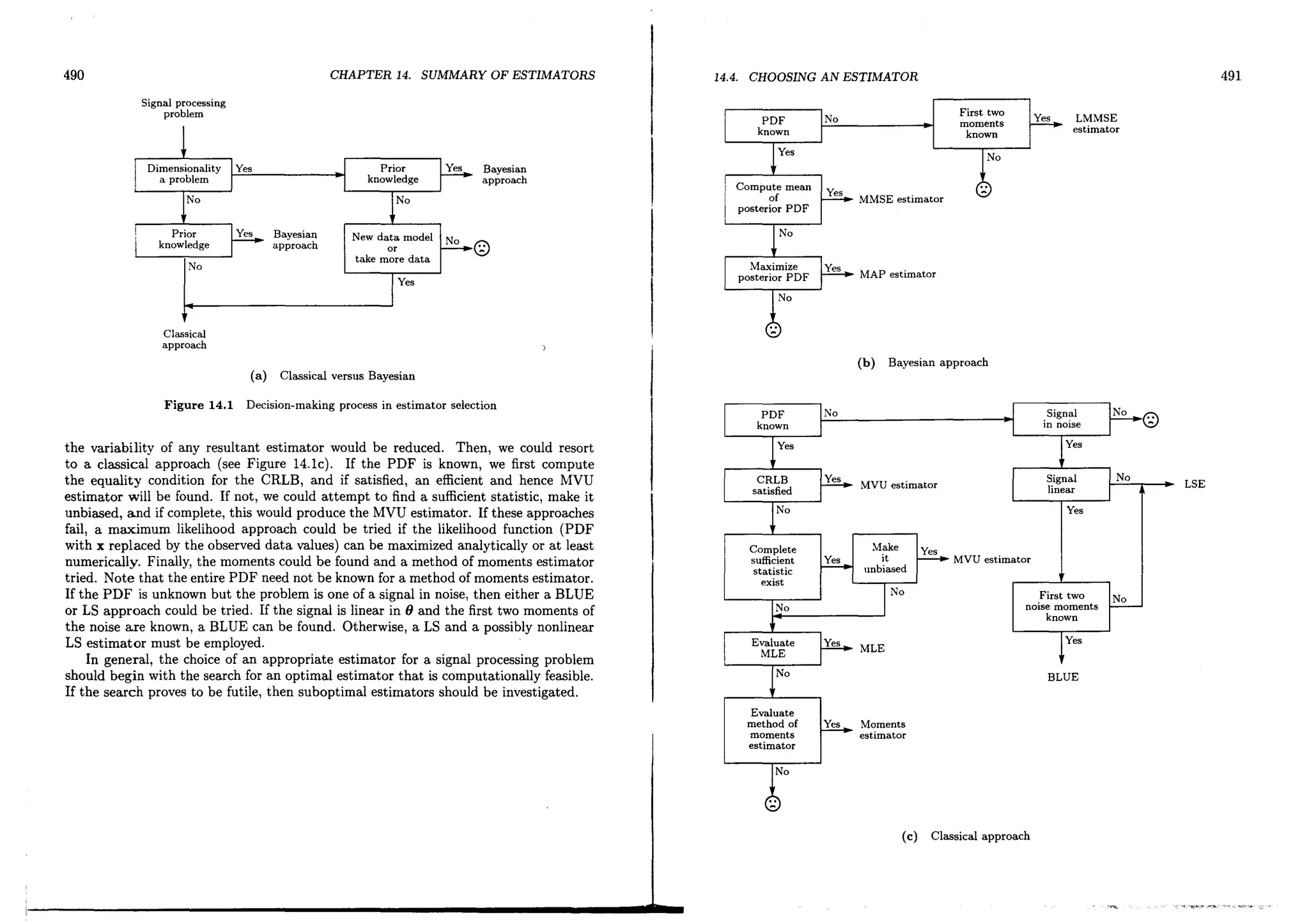
![494 CHAPTER 15. COMPLEX DATA AND PARAMETERS
S(F) S(F)
-Fa Fa - ~ Fa Fa + ~
F (Hz) F (Hz)
(a) Fourier transform of real bandpass signal (b) Fourier transform of complex envelope
Figure 15.1 Definition of complex envelope
of (15.19) or, equivalently, the covariances satisfy (15.20) for the case of two random
variables. Properties of complex Gaussian random variables are summarized iIi' that
section as well. If a complex WSS random process has an autocorrelation and a cross-
correlation that satisfy (15.33), then it is said to be a complex Gaussian WSS random
process. An example is the complex envelope of a real bandpass Gaussian random
process, as described in Example 15.5. The complex derivative of a real function with
respect to a complex variable is formally defined in (15.40). The associated complex
gradient can be used to minimize Hermitian functions by employing (15.44)-(15.46).
If the Hermitian function to be minimized has a linear constraint on its parameters,
then the solution is given by (15.51). Classical estimation based on complex Gaussian
data with real parameters employs the CRLB of (15.52) and the equality condition of
(15.53). When the Fisher information matrix has a special form, however, the equality
condition of (15.54) can be used. This involves a complex Fisher information matrix.
One important example is the complex linear model in Example 15.9, in which (15.58)
ts the efficient estimator and (15.59) is its corresponding covariance. Bayesian estima-
tion for the complex Bayesian linear model is discussed in Section 15.8. The MMSE
estimator is given by (15.64) or (15.65), while the minimum Bayesian MSE is given by
(15.66) or (15.67). For large data records an approximate PDF for a complex Gaussian
WSS random process is (15.68) and an approximate CRLB can be computed based on
(15.69). These forms are frequently easier to use in deriving estimators.
15.3 Complex Data and Parameters
The most common example of the use of complex data in signal processing occurs in
radar/sonar in which a bandpass signal is of interest. As shown in Figure 15.1a, if the
Fourier transform S(F) of a continuous-time real signal s(t) is nonzero over a band (Fo-
B/2, Fa +B/2), then the essential information is contained in the complex envelope s(t)
whose Fourier transform S(F) is shown in Figure 15.1b. (We will generally use a tilde
to denote a complex quantity when necessary to avoid confusion. Otherwise, whether
the quantity is real or complex will be evident from the context of the discussion.) The
15.3. COMPLEX DATA AND PARAMETERS 495
set)
sin 271'Fat
(quadrature)
B F
'2
Fs=!"=B
~
s(n~) = sIn]
,
-. - --- ----- --- -- -- -- ------ - -- ----
Within digital computer
Figure 15.2 Extraction of discrete-time complex envelope from bandpass signal
relationship between the Fourier transforms of the real bandpass signal and its complex
envelope is
S(F) = S(F - Fa) + S*(-(F + Fa)). (15.1)
To obtain S(F) we shift the complex envelope spectrum up to F = Fa and also, after
first "flipping it around" in F and conjugating it, down to F = -Fa. Taking the
inverse Fourier transform of (15.1) produces
s(t) = s(t) exp(j2nPot) + [s(t) exp(j27l'Fot)]*
or
s(t) = 2Re [s(t) exp(j27l'Fot)]. (15.2)
Alternatively, if we let s(t) = SR(t) + jSJ(t), where R and I refer to the real and
imaginary parts of the complex envelope, we have
(15.3)
This is also referred to as the "narrowband" representation, although it is actually
valid if Fa > B/2. Note that SR(t),SJ(t) are bandlimited to B/2 Hz, as is evident
from Figure 15.1b. Hence, the bandpass signal is completely described by its complex
envelope. In processing s(t) or a noise corrupted version we need only obtain the
complex envelope. From a practical viewpoint the use of the complex envelope, which
is a low-pass signal, allows us to sample at the lower rate of B complex samples/sec
as opposed to the higher rate of 2(Fo + B/2) real samples/sec for the real bandpass
signal. This results in the widely adopted means of processing a real bandpass signal
shown in Figure 15.2. The aim is to produce the samples of the complex envelope
in a digital computer. Note from (15.3) that the output of the low-pass filter for the](https://image.slidesharecdn.com/fundamentalsofstatisticalsignalprocessing-estimationtheory-kay-230513154707-1f7652e0/75/Fundamentals-Of-Statistical-Signal-Processing-Estimation-Theory-Kay-pdf-253-2048.jpg)
![496 CHAPTER 15. COMPLEX DATA AND PARAMETERS
"in-phase" channel is
[2sR(t) COS
221TFat - 2sI(t) sin 21TFot cos 21TFat] LPF
[SR(t) + SR(t) cos 41TFot - SI(t) sin 41TFot]LPF
= SR(t)
since the other signals have spectra centered about ±2F
o. The "LPF" designation
means the output of the low-pass filter in Figure 15.2. Similarly, the output of the
low-pass filter in the "quadrature" channel is SI(t). Hence, the discrete signal at the
output of the processor in Figure 15.2 is sR(n~) +jSI(n~) = s(n~). It is seen that
complex data naturally arise in bandpass systems. An important example follows.
Example 15.1 - Complex Envelope for Sinusoids
It frequently occurs that the bandpass signal of interest is sinusoidal, as for example,
p
s(t) = L Ai COS(21TFit +<Pi)
i=l
where it is known that Fo - B /2 :S Fi :S Fo + B /2 for all i. The complex envelope for
this signal is easily found by noting that it may be written as
S(t) = Re [tAi exp [j(21TFit +<Pi)]]
2Re [t~i exp [j(21T(Fi - Fo)t +<Pi)] eXp[j21TFot]]
so that from (15.2)
p A
s(t) = L -;f exp(j<Pi) exp[j21T(Fi - Fo)t].
i=l
:-.rote that the complex envelope is composed of complex sinusoids with frequencies
F; - Fo, which may be positive or negative, and complex amplitudes ~ exp(j<Pi). If we
sample at the Nyquist rate of Fs = 1/~ = B, we have as our signal data
p A
s(n~) = L -;f exp(j<Pi) exp(j21T(Fi - Fo)n~].
i=l
Furthermore, we can let s[n] = s(n~), so that
p
s[n] = L Ai exp(j21Tj;n)
i=l
J
15.3. COMPLEX DATA AND PARAMETERS 497
where Ai = ~ exp(j<Pi) is the complex amplitude and fi = (Fi - Fo)~ is the frequency
of the ith discrete sinusoid. For the purposes of designing a signal processor we may
assume the data model
p
x[n] = L Ai exp(j21Tfin) +w[n]
i=l
where w[n] is a complex noise sequence. This is a commonly used model. o
A complex signal can also arise when the analytic signal sa(t) is used to represent a
real low-pass signal. It is formed as
sa(t) = s(t) + j1£[s(t)]
where 1£ denotes the Hilbert transform [Papoulis 1965]. The effect of forming this
complex signal is to remove the redundant negative frequency components of the Fourier
transform. Hence, if S(F) is bandlimited to B Hz, then Sa(F) will have a Fourier
transform that is zero for F < 0 and so can be sampled at B complex samples/sec. As
an example, if
p
s(t) = L Ai COS(21TFit + <Pi)
i=l
then it can be shown that
p
Sa(t) = L Ai exp [j(21TFit + <Pi)].
i=l
Now that the use of complex data has been shown to be a natural outgrowth of
bandpass signal processing, how do complex parameters come about? Example 15.1
illustrates this possibility. Suppose we wanted to estimate the amplitudes and phases
of the p sinusoids. Then, a possible parameter set would be {AI> <PI> A2,<P2, ... , Ap , <pp},
which consists of 2p real parameters. But, equivalently, we could estimate the complex
parameters {AI exp(j<PI), A2 exp(j<p2), ... , Ap exp(j<pp)}, which is only a p-dimensional
but complex parameter set. The equivalence of the two parameter sets is evident from
the transformation
A = Aexp(j¢)
and inverse transformation
A
Another common example where complex parameters occur is in spectral modeling of
a nonsymmetric PSD. For example, an AR model of the PSD of a complex process x[n]
would assume the form [Kay 1988]
(j2
Pxx(f) = u 2.
11 +a[l] exp(-j21Tf) + ... +a[p] exp(-j21Tfp)I](https://image.slidesharecdn.com/fundamentalsofstatisticalsignalprocessing-estimationtheory-kay-230513154707-1f7652e0/75/Fundamentals-Of-Statistical-Signal-Processing-Estimation-Theory-Kay-pdf-254-2048.jpg)
![498 CHAPTER 15. COMPLEX DATA AND PARAMETERS
If the PSD is nonsymmetric about f = 0, corresponding to a complex ACF and thus a
complex random process [Papoulis 1965], then the AR filter parameters {a[l]' a[2], ... ,
alP]} will be complex. Otherwise, for real a[kJ's we would have Pii(- f) = Pii(f). It
seems, therefore, natural to let the filter parameters be complex to allow for all possible
spectra.
In dealing with complex data and/or complex parameters we can always just decom-
pose them into their real and imaginary parts and proceed as we normally would for
real data vectors and/or real parameter vectors. That there is a distinct disadvantage
in doing so is illustrated by the following example.
Example 15.2 - Least Squares Estimation of Amplitude
Suppose we wish to minimize the LS error
N-l
J(A) = 2:= Ix[n] - As[n]i2
n=O
over A, where x[n], A, s[n] are all complex. A straightforward approach would decom-
pose all complex quantities into their real and imaginary parts to yield
N-l
J'(AR,AI) = 2:= IXR[n] + jXI[n]- (AR + jAI )(sR[n] + jSI[n]W
n=O
N-l
2:=(xR[n]- ARSR[n] + ArsIln])2 + (xr[n]- ARsr[n]- AIsR[n])2.
n=O
This is a standard quadratic form in the real variables AR and AI. Hence, we can let
XR = [XR[O] xR[l] ... xR[N - lW, XI = [xIlO] xIl1] ... xI[N - lW, SR = [SR[O] sR[l] ...
sR[N - lW, SI = [sr[O] sI[l] ... sIlN - 1]JT, so that
J'(AR,AI) = (XR - ARsR + ArSI)T(XR - ARsR+ AIsr)
+ (Xr - ARsI - AIsRl(XI - ARsI - AIsR)
or letting SI = [SR - SI], S2 = lSI SR], and A = [AR AI]T
J' (A) (XR - sIA)T(XR - SIA) + (XI - s2A)T (XI - S2A)
X~XR - x~slA - ATsfXR + ATsfSIA
+ xfXI - xfS2A - ATsfXI + ATsfs2A.
Taking the gradients and using (4.3) yields
15.3. COMPLEX DATA AND PARAMETERS
Setting this equal to zero and solving produces
A (SfSl+sfs2)-I(sfxR+sfxI)
([
Sk:R -~kSI] + [ S~SI
-SI SR SI SI SRSI
[
SkXR + SjXI
SkSR + SjSI
SkXI - SjXR
SkSR + SjSI
499
which i~ the minimizing solution. However, if we rewrite Ain complex form as AR +
JAI = A, we have
SkXR + sjXI + jSkXI - JSJXR
SkSR + sjSI
(XR + jXIf (SR - jSI)
SkSR + SJSI
N-l
2:=x[n]s*[n]
n=O
N-l
2:= Is[nW
n=O
a result analogous to the real case. We can simplify the minimization process using
complex variables as follows. First, define a complex derivative as (see Section 15.6 for
further discussions) [Brandwood 1983]
oj 1 (OJ . oj )
oA = 2 OAR - J OAI
and note that
:~ = 0 if and only if :~ = O.
Then, we must establish that (see Section 15.6 for the definition of a derivative of a
complex function)
oA
8A
1 (15.4)](https://image.slidesharecdn.com/fundamentalsofstatisticalsignalprocessing-estimationtheory-kay-230513154707-1f7652e0/75/Fundamentals-Of-Statistical-Signal-Processing-Estimation-Theory-Kay-pdf-255-2048.jpg)
![500 CHAPTER 15. COMPLEX DATA AND PARAMETERS
aA*
aA
aAA*
aA
o
-aA* aA- -
A-_ + -_A* = A*
aA aA
(15.5)
(15.6)
as we shall do in Section 15.6. Now, we can minimize J using the complex derivative
aJ
aA
a N-l
-- L Ix[n]- As[n]1
2
aA n=O
tl~ (lx[nW - x[n]A*s*[n]- As[n]x*[n] + AA*ls[nW)
n=O aA
N-l
L (0 - 0 - s[n]x*[n] + A*ls[nW).
n=O
)
Setting this equal to zero and solving produces the same results. Thus, we see that
with the use of some easily established identities the algebra required for minimization
becomes quite simple. 0
15.4 Complex Random Variables and PDFs
As we have seen, it is quite natural to encounter complex signal models. To formulate
complex noise models as well we now extend many of our standard definitions and
results for real random variables to complex ones. A complex random variable x is
defined to be x= U+jv, where u, v, the real and imaginary parts of x, are real random
variables. The tilde denotes a complex random variable since we will have need to
distinguish it from a real random variable. We will assume that the real random vector
[uvf possesses a joint PDF, allowing us to define moments of the complex random
variable. The mean of xis defined as
E(x) = E(u) + jE(v) (15.7)
where the expectation is with respect to the marginal PDFs or p(u) and p(v), and the
second moment is defined as
(15.8)
The variance is defined as
var(X) = E (Ix - E(xW) (15.9)
which can easily be shown to reduce to
(15.10)
I
...
15.4. COMPLEX RANDOM VARIABLES AND PDFS 501
If we now have two complex random variables Xl and X2 and a joint PDF for the real
random vector [Ul U2 VI v2f, then we can define a cross-moment as
E [(Ul - jVI)(U2 + jV2)]
[E(UlU2) + E(VlV2)] +j [E(UlV2) - E(U2Vl)]
which is seen to involve all the possible real cross-moments. The covariance between
Xl and X2 is defined as
(15.11)
and can be shown to reduce to
(15.12)
Just as in the real case, if Xl is independent of X2, which is to say [Ul vlf is independent
of [U2V2f, then COV(Xl,X2) = 0 (see Problem 15.1). Note that the covariance reduces
to the variance if Xl = X2. We can easily extend these definitions to complex random
vectors. For example, if x= [Xl X2 ... xnf, then the mean of xis defined as
and the covariance of xis defined as
l
var(xI)
COV(~2' Xl)
COV(Xm Xl)
COV(Xb X2)
var(x2)
... COV(Xl' xn) j*
·.. COV(X2, xn)
· .
. .
. .
·. . var(xn)
(15.13)
where H denotes the conjugate transpose of a matrix. Note that the covariance matrix is
Hermitian or the diagonal elements are real and the off-diagonal elements are complex
conjugates of each other so that Cf = CX. Also, Cx can be shown to be positive
semidefinite (see Problem 15.2).
We frequently need to compute the moments of linear transformations of random
vectors. For example, if y = Ax + b, where x is a complex n x 1 random vector, A is](https://image.slidesharecdn.com/fundamentalsofstatisticalsignalprocessing-estimationtheory-kay-230513154707-1f7652e0/75/Fundamentals-Of-Statistical-Signal-Processing-Estimation-Theory-Kay-pdf-256-2048.jpg)
![502 CHAPTER 15. COMPLEX DATA AND PARAMETERS
a complex m x n matrix, b is a complex m x 1 vector, so that y is a complex m x 1
random vector, then
E(y) = AE(i) +b
Cy = ACxAH.
The first result follows from considering
so that
n
Yi = 2)A]ijXj + bi
j=l
n
E(fji) = ~)A]ijE(xj) + bi
j=l
and expressing the results in matrix form. The second result uses the first to yield
Cy E [(y - E(y))(y - E(y))H]
= E [A(i - E(i))(i - E(i))H AH].
But
E {[A(i - E(i))(i - E(i))HAHLj
}
E {~t[A]ik[(i - E(i))(i - E(i))H]k/[AH]/j }
n n
L L[A]idCx]kdAH]lj
k=ll=l
and expressing this in matrix form yields the desired result. It is also of interest to
determine the first two moments of a positive definite Hermitian form or of
Q =iHAi
where i is a complex n x 1 random vector and A is an n x n positive definite hermitian
(AH = A) matrix. Note that Q is real since
(iHAi)H
iHAHi
iHAi
Q.
Also, since A is assumed to be positive definite, we have Q > 0 for all i # O. To find
the moments of Q we assume E(x) = o. (If this is not the case, we can easily modify
the results by replacing x by y = x - E(x) and then evaluating the expressions.) Thus,
E(Q) E(iHAx)
= E(tr(AiiH))
I
~
15.4. COMPLEX RANDOM VARIABLES AND PDFS
E(Q) tr[E(AiiH)]
tr[AE(xxH)]
tr(ACx).
To find the second moment we need to evaluate
503
(15.14)
(15.15)
which will require fourth-order moments of x (see Example 15.4). Recall that for a
real Gaussian PDF the fourth-order moments were functions of second-order moments,
considerably simplifying the evaluation. We will show next that we can define a complex
Gaussian PDF for complex random variables and that it will have many of the same
properties as the real one. Then, we will be able to evaluate complicated expressions
such as (15.15). Furthermore, the complex Gaussian PDF arises naturally from a
consideration of the distribution of the complex envelope of a bandpass process.
We begin our discussion by defining the complex Gaussian PDF of a scalar complex
random variable x. Since x = u + jv, any complete statistical description will involve
the joint PDF of u and v. The complex Gaussian PDF assumes u to be independent
of v. Furthermore, it assumes that the real and imaginary parts are distributed as
N(/-LUl u2
/2) and N(/-Lv, u2
/2), respectively. Hence, the joint PDF of the real random
variables becomes
p(u,v)
But letting jj = E(x) = /-Lu + j/-Lv, we have in more succinct form
(15.16)
Since the joint PDF depends on u and v only through x, we can view the PDF to be that
of the scalar random variable x, as our notation suggests. This is called the complex
Gaussian PDF for a scalar complex random variable and is denoted by CN(jj, ( 2
). Note
the similarity to the usual real Gaussian PDF. We would expect p(x) to have many of
the same algebraic properties as the real Gaussian PDF, and indeed it does. To extend
these results we next consider a complex random vector i = [Xl X2 ... xnf. Assume
the components of x are each distributed as CN(jji, un and are also independent. By
independence we mean that the real random vectors [Ul vdT
, [U2 v2f, ... , [un vnf are](https://image.slidesharecdn.com/fundamentalsofstatisticalsignalprocessing-estimationtheory-kay-230513154707-1f7652e0/75/Fundamentals-Of-Statistical-Signal-Processing-Estimation-Theory-Kay-pdf-257-2048.jpg)
![504 CHAPTER 15. COMPLEX DATA AND PARAMETERS
independent. Then, the multivariate complex Gaussian PDF is just the product of the
marginal PDFs or
n
p(i) = ITp(Xi)
t=1
which follows from the usual property of PDFs for real independent random variables.
From (15.16) this can be written as
p(i) = 7rn n~ a2 exp [- t :2lxi - iii12] .
t=1 1 l=l l
But noting that for independent complex random variables the covariances are zero,
we have the covariance matrix for i
ex = diag(a~, a~, ... , a~)
so that the PDF becomes
(15.17)
This is the multivariate complex Gaussian PDF. and it is denoted by CN(jL, ex). Again
note the similarity to the usual real multivariate Gaussian PDF. But (15.17) is more
general than we have assumed in our derivation. It is actually valid for complex covari-
ance matrices other than just diagonal ones. To define the general complex Gaussian
PDF we need to restrict the form of the underlying real covariance matrix, as we now
show. Recall that for a scalar complex Gaussian random variable x = U + jv the real
covariance matrix of [u vJT is
For a 2 x 1 complex random vector i = [XI x2l
T
= [UI + jVI U2 + jV2]Y with XI inde-
pendent of X2, as we have assumed, the real covariance matrix of [UI VI U2 V2]Y is
[
ai 0 0 0 1
~ 0 ai 0 0
2 0 0 a~ 0 .
o 0 0 ai
If we rearrange the real random vector as x = [UI U2 VI v2lT, then the real covariance
matrix becomes
o
o
o
o
o
(15.18)
J
15.4. COMPLEX RANDOM VARIABLES AND PDFS 505
This is a special case of the more general form of the real 4 x 4 covariance matrix
1[A -B]
ex = 2" B A (15.19)
where A and B are each 2 x 2 matrices. This form of ex allows us to define a complex
Gaussian PDF for complex Gaussian random variables that are correlated. By letting
u = [Ul U2JT and v = [VI V2JT we see that the submatrices of ex are
~A E[(u - E(u))(u - E(u)fl = E[(v - E(v))(v - E(v)fl
2
~B E[(v - E(v))(u - E(u)fl = -E[(u - E(u))(v - E(v)fl.
2
Thus A is symmetric and B is skew-symmetric or BT = -B. Explicitly, the real
covariance matrix is
[
var(ul) COV(Ul,U2) I cOV(UJ,Vl)
cov(U2, ud var(U2) I cov(U2, vd
ex = - - -- - - -- I - - --
cov(VI, ud cov(VI, U2) I var(VI)
COV(V2,Ul) COV(V2,U2) I COV(V2,Vl)
COV(Ul,V2)
cov(U2, V2)
COV(Vl,V2)
var(V2)
For ex to have the form of (15.19) we require (in addition to variances being equal or
var(ui) = var(vi) for i = 1,2, and the covariance between the real and imaginary parts
being zero or cov(Ui, Vi) = 0 for i = 1,2, as we have assumed for the scalar complex
Gaussian random variable) the covariances to satisfy
COV(Ul,U2)
COV(Ul, V2)
COV(Vl,V2)
- COV(U2, VI)' (15.20)
The covariance between the real parts is identical to that between the imaginary parts,
and the covariance between the real part of Xl and the imaginary part of X2 is the
negative of the covariance between the real part of X2 and the imaginary part of Xl'
With this form of the real covariance matrix, as in (15.19), we can prove the following
(see Appendix 15A) for i = [Xl X2 ••• xnl = [Ul + jVl U2 + jV2 ••. Un + jVnJT and for
A and B both having dimensions n x n.
1. The complex covariance matrix of i is ex = A + jB. As an example, for n = 2
and independent XI, X2, ex is given by (15.18) and thus
ex = A +jB = A = [~i ~~].
2. The quadratic form in the exponent of the real multivariate Gaussian PDF may
be expressed as](https://image.slidesharecdn.com/fundamentalsofstatisticalsignalprocessing-estimationtheory-kay-230513154707-1f7652e0/75/Fundamentals-Of-Statistical-Signal-Processing-Estimation-Theory-Kay-pdf-258-2048.jpg)
![506 CHAPTER 15. COMPLEX DATA AND PARAMETERS
where [L = E(i) = I'u +jl'v' As an example, for n = 2 and independent Xll X2,
we have from (15.18) and (15.19)
so that
C, ~ [! ~1
T [ A-I 0 ] [ u - I'u ]
[ (u - I'uf (v - I'v)]2 0 A-I V _ I'v
2[(u - I',,)TA-l(U - I'u)] + [(v - I'vfA-l(V - I'v)]
2[(u - I'u) - j(v - I'vWCi l
[(u - 1',,) +j(v - I'v)]
2(i - [L)HCil(i - [L)
since Cx = A, where A is real.
3. The determinant of Cx is
Note that det(Cx) is real and positive since Cx is Hermitian and positive definite.
As an example, for n = 2 and independent Xl, X2 we have Cx = A, and from
(15.18) and (15.19)
so that
With these results we can rewrite the real multivariate Gaussian PDF of
x =[Ul '" Un VI ••• Vn]T
I
J
15.4. COMPLEX RANDOM VARlABLES AND PDFS 507
as
p(x) p(i)
1 [(- -)HC-l (- _)]
d (C)
exp - X - I' x X - I'
1l'n et x
where [L is the mean and Cx is the covariance matrix of i. Whereas the real Gaussian
PDF involves 2n x 1 real vectors and 2n x 2n real matrices, the complex Gaussian PDF
involves n x 1 complex vectors and n x n complex matrices. We now summarize our
results in a theorem.
Theorem 15.1 (Complex Multivariate Gaussian PDF) If a real random vector
X of dimension 2n x 1 can be partitioned as
where u, v are real random vectors and x has the PDF
and Cuu = Cvv and Cuv = -Cvu 01'
cov(U;, uJ )
COV(Ui,Vj)
cov(V;, vJ )
-COV(Vi,Uj) (15.21)
then defining the nx 1 complex random vector i = u+jv, i has the complex multivariate
Gaussian PDF
i "" CN([L, Cx)
where
[L I'u+jl'v
Cx 2(Cuu + jCvu)
01' more explicitly
(15.22)
It is important to realize that the complex Gaussian PDF is actually just a different
algebraic form of the real Gaussian PDF. What we have essentially done is to replace
2 x 1 vectors by complex numbers or [u vf --+ X = U +jv. This will simplify subsequent
estimator calculations, but no new theory should be expected. The deeper reason that
allowed us to perform this trick is the isomorphism that exists between the vector
spaces M2 (the space of all special 2 x 2 real matrices) and Cl
(the space of all complex](https://image.slidesharecdn.com/fundamentalsofstatisticalsignalprocessing-estimationtheory-kay-230513154707-1f7652e0/75/Fundamentals-Of-Statistical-Signal-Processing-Estimation-Theory-Kay-pdf-259-2048.jpg)
![508 CHAPTER 15. COMPLEX DATA AND PARAMETERS
numbers). We can transform matrices from M2 to complex numbers in Cl, perform
calculations in Cl
, and after we're done transform back to M2. As an example, if we
wish to multiply the matrices
we can, equivalently, multiply the complex numbers
(a + jb)(e + jf) = (ae - bf) + j(aJ + be)
and then transform back to M2. We will explore this further in Problem 15.5.
There are many properties of the complex Gaussian PDF that mirror those of the
real one. We now summarize the important properties with the proofs given in Ap-
pendix 15B.
1. Any subvector of a complex Gaussian random vector is also complex Gaussian.
In particular, the marginals are complex Gaussian.
2. If i = [:i X2'" xnJT is complex Gaussian and {Xl' X2,"" xn} are uncorrelated,
then they are also independent.
3. If {Xl,X2,'" ,Xn} are independent, each one being complex Gaussian, then i =
[Xl X2 .•. xnJT is complex Gaussian.
4. Linear (actually affine) transformations of complex Gaussian random vectors are
again complex Gaussian. More specifically, if y = Ai + b, where A is a complex
m x n matrix with m ~ n and full rank (so that Cjj is invertible), b is a complex
m x 1 vector, and if i '" eN(jL, Cx), then
y '" eN(AjL +b, ACxAH). (15.23)
5. The sum of independent complex Gaussian random variables is also complex Gaus-
sian.
6. If i = [Xl X2 X2 X4JT '" eN(o, Cx), then
E(X~X2X;X4) = E(X~X2)E(x;X4) + E(X~X4)E(X2X;), (15.24)
It is interesting to note that E(xix;) = E(X2X4) = 0 (as we will show shortly), so
that this result is analogous to the real case, with the last product being equal to
zero.
1. If [iT yT]T is a complex Gaussian random vector, where i is k x 1 and y is I x 1
and
eN Cxx Cxy
[
i ] ([ E(i) ] )
y '" E(y) , [Cyx Cyy ]
j
15.4. COMPLEX RANDOM VARIABLES AND PDFS
then the conditional PDF p(Yli) is also complex Gaussian with
E(y) + cyxCii (i - E(i))
Cyy - cjjxciicxjj'
This is identical in form to the real case (see (10.24) and (10.25)).
509
(15.25)
(15.26)
These properties appear reasonable, and the reader will be inclined to accept them.
The only one that seems strange is property 6, which seems to imply that for a zero
mean complex Gaussian random vector we have E(XIX2) = O. To better appreciate
this conjecture we determine this cross-moment as follows:
E[(UI +jVl)(U2 + jV2)]
E(UIU2) - E(VIV2) +j[E(UIV2) + E(VIU2)]
COV(Ub U2) - COV(Vl' V2) + j[COV(Ul, V2) +COV(U2' VI)]
which from (15.20) is zero. In fact, we have actually defined E(XIX2) = 0 in arriving
at the form of the covariance matrix in (15.19) (see Problem 15.9). It is this constraint
that leads to the special form assumed for the real covariance matrix. We will now
illustrate some of the foregoing properties by applying them in an important example.
Example 15.3 - PDF of Discrete Fourier Transform of WGN
Consider the real data {x[O],x[IJ, ... ,x[N - I]} which are samples of a WGN process
with zero mean and variance (J2/2. We take the discrete Fourier transform (DFT) of
the samples to produce
N-l
X(fk) = L x[n] exp(-j27l"Jkn)
n=O
for Jk = k/Nand k = 0, 1, ... ,N - 1. We inquire as to the PDF of the complex DFT
outputs for k = 1,2, ... , N/2 - 1, neglecting those for k = N/2 + 1, N/2 +2, ... , N - 1
since these are related to the chosen outputs by X(fk) = X*(fN-k). We also neglect
X(fo) and X(fN/2) since these are purely real and ar~ usually of little intere~t anyway,
occurring at DC and at the Nyquist frequency. We WIll show that the PDF IS
(15.27)
To verify this we first note that the real random vector
[Re(X(fd) ... Re(X(f!f-l)) Im(X(fl))](https://image.slidesharecdn.com/fundamentalsofstatisticalsignalprocessing-estimationtheory-kay-230513154707-1f7652e0/75/Fundamentals-Of-Statistical-Signal-Processing-Estimation-Theory-Kay-pdf-260-2048.jpg)
![510 CHAPTER 15. COMPLEX DATA AND PARAMETERS
is a real Gaussian random vector since it is a linear transformation of x. Thus, we need
only show that the special form of the real covariance matrix of X is satisfied. First,
we show that the real and imaginary parts of X(fk) are uncorrelated. Let X(Jk) =
U(/k) +jV(/k), where U and V are both real. Then
N-l
U(M L x[n] cos 27rAn
n=O
N-l
V(/k) - L x[n] sin 27rfkn
n=O
and therefore
N-l
E(U(/k)) = L E(x[n]) cos 27rfkn = 0
n=O
and similarly E(V(/k)) = O. Now
cov(U(A), U(ft)) E(U(Jk )U(ft))
E [%=:~x[m]x[n] cos 27rAmCOS27rf1n]
N-l N-l 2
L L ~ o[m-n]cos27rfkmCos27r!In
m=O n=O
2 N-l
~ L cos 27rfknCOS 27rfln
n=O
2 N-l 1
~ L"2 [cos 27r(Jk +ft)n +cos 27r(Jk - fl)n]
n=O
2 N-l
~ L cos 27r(fk - fl)n
n=O
due to the DFT relation in Appendix 1. Now if fk 1= fI, COV(U(Jk), U(Jd) = 0 by
the same DFT relation. If A = f/, we have COV(U(Jk),U(Jk)) = Na2/4. A similar
calculation shows that
and so
Na2
Cuu = Cvv = --I
4
15.4. COMPLEX RANDOM VARIABLES AND PDFS 511
as required. To verify that Cuv = -Cvu we show that these are both zero.
E(U(/k)V(ft))
E (%~x[m]x[n] cos 27r/km sin 27r!In)
2 N-l
~ Leos 27rfkn sin 27rfm
n=O
o for all k,l
by the DFT relation in Appendix 1. Similarly, COV(V(fk), U(ft)) = 0 for all k, l. Hence,
Cuv = -Cvu = o. From Theorem 15.1 the complex covariance matrix becomes
Cx 2(Cuu + jCvu )
Na2
- I
2
and the assertion is proved. Observe that the DFT coefficients are independent and
identically distributed. As an application of this result we may wish to estimate a2
using
1!-1
;2 =! t IX(fkW.
c k=l
This is frequently required for normalization purposes in determining a threshold for a
detector [Knight, Pridham, and Kay 1981]. For the estimator to be unbiased we need
to choose an appropriate value for c. But
1!-1
E(;2) = ! t E(IX(fkW)·
c k=l
Since X(fk)""" CN(O,Na2
/2), we have that
and
Hence, c should be chosen to be N(N/2 -1)/2. o](https://image.slidesharecdn.com/fundamentalsofstatisticalsignalprocessing-estimationtheory-kay-230513154707-1f7652e0/75/Fundamentals-Of-Statistical-Signal-Processing-Estimation-Theory-Kay-pdf-261-2048.jpg)
![512 CHAPTER 15. COMPLEX DATA AND PARAMETERS
Example 15.4 - Variance of Hermitian Form
As a second application, we now derive the variance of the Hermitian form
Q =xHAx
where x '" CN(O, Cx) and A is Hermitian. The mean has already been given in (15.14)
as tr(ACx). We first determine the second moment
n n n n
L L L L[A]ij[A]kIE(X;XjXZxt).
i=1 j=1 k=1 1=1
Using the fourth-order moment property (15.24), we have
Thus,
But
E(x:Xj)E(x~XI) +E(x:xI)E(x~Xj)
[CIJ;j[Cf]kl + [CIlil[cf]kj.
n n n n
i=1 j=1 k=1 1=1
n n n n
i=1 j=1 k=1 1=1
n n n n
L L[CIJ;j [A]ij L L[CTlkt[A]kl
i=1 )=1 k=II=1
(15.28)
where a;, hi are the ith columns of A and B, respectively. More explicitly this becomes
I
I
J
15.5. COMPLEX WSS RANDOM PROCESSES 513
tr(BTA)
n n
i=1 j=1
n n
L L[B]ij[A]ij
i=1 j=1
so that the first term in (15.28) is just tr2(CxA) or tr2(ACx), the squared mean. Let
D = ACx. Then, the second term is
n n n n
L L[D]idD]ki = L L[DT]ki[D]ki
i=1 k=1 k=li=1
which is
tr(DD) = tr(ACxACx)
so that finally we have for x '" CN(O, Cx) and A Hermitian
E(XHAx)
var(xH
Ax)
tr(ACx)
tr(ACxACx)·
An application of this result is given in Problem 15.10.
15.5 Complex WSS Random Processes
(15.29)
(15.30)
o
We are now in a position to discuss the statistical modeling of the complex random
process x[n] = urn] + jv[n]. It will be assumed that x[n] is WSS, which, as for real
processes, implies that the mean does not depend on n and the covariance between x[n]
and x[n + k] depends only on the lag k. The mean is defined as
E(x[n]) = E(u[n]) + jE(v[n])
and will be assumed to be zero for all n. Since x[n] is WSS, we can define an ACF as
Txx[k] = E(x*[n]x[n + k]) (15.31)
and as usual the PSD is the Fourier transform of Txx[k]. If the random vector formed
from any subset of samples, say {x[nd, x[n2], ... ,x[nk]}, has a multivariate complex
Gaussian PDF, then we say that x[n] is a WSS complex Gaussian random process. Its](https://image.slidesharecdn.com/fundamentalsofstatisticalsignalprocessing-estimationtheory-kay-230513154707-1f7652e0/75/Fundamentals-Of-Statistical-Signal-Processing-Estimation-Theory-Kay-pdf-262-2048.jpg)
![514
CHAPTER 15. COMPLEX DATA AND PARAMETERS
comp~ete statist~cal description is then summarized by the ACF, which determines the
covariance matnx, or, equivalently, by the PSD (since the mean is zero). Since the
real co~iance matrix i~ constrained to be of the form (15.19), this translates into a
constraillt on rxx[kJ. To lllterpret this constraint recall that we require
Cuu = Cvv
Cuv = -Cvu
for all u = [u[nd··· u[nkW and v = [v[nd ... v[nkW. This means that
E(u[niJu[nj]) = E(v[niJv[njJ)
E(u[niJv[njJ) = - E(v[niJu[njJ)
for all i: j: By defining the ACF of x[nJ it is implicit that urn], v[nJ are both WSS, as
well as JOllltly WSS. If we define the cross-correlation function (CCF) as
then we must have
ruv[kJ = E(u[nJv[n + kJ)
ruu[kJ = rvv[kJ
ruv[kJ = -rvu[kJ
for all k, where we have let k = nj - ni. Alternatively, we require
Puu(f) = Pvv(f)
Puv(f) = - Pvu (f)
)(15.32)
(15.33)
(15.34)
where Puu(f), Pvv(f) are the auto-PSDs and Puv(f), Pvu(f) are the cross-PSDs. Since
the cro~s:PSDs are complex conjugates of each other, the second condition is equivalent
to req~Iring the cross-PSD to be purely imaginary. Then, if u[nJ, v[nJ are real jointly
Gaussian rando~ processes with zero mean and PSDs satisfying (15.34), x[nJ will be
a complex Gaussian random process. Furthermore, the PSD of x[nJ can be related to
those of u[nJ and v[nJ as follows. From (15.31) and (15.33)
rxx[kJ = E [(u[nJ - jv[nJ)(u[n + kJ + jv[n + kJ)]
= ruu[kJ + jruv[kJ - jrvu[kJ + rvv[kJ.
But from (15.33) this reduces to
and thus
(15.35)
Pxx(f) = 2(Puu(f) + jPuv(f)). (15.36)
The reader at this point may recognize that the same relationships (15.33) and (15.34)
occur for a process and its Hilbert transform or the real and imaginary parts of a
15.5. COMPLEX WSS RANDOM PROCESSES 515
bandpass noise process. Thus, the complex envelope or the analytic signal of a WSS
Gaussian random process is a complex WSS Gaussian random process (see Problem
15.12). Since these results are standard fare in many textbooks [Papoulis 1965J, we
only briefly illustrate them. We consider a bandpass noise process using the complex
envelope representation. What we will show is that by concatenating the in-phase
and quadrature processes together into a single complex envelope process, a complex
WSS Gaussian random process results if the bandpass process is a real WSS Gaussian
process.
Example 15.5 - Bandpass Gaussian Noise Process
Consider a real continuous bandpass WSS Gaussian process x(t) with zero mean. It
can be represented by its complex envelope as (using an argument similar to that in
Section 15.3 but replacing Fourier transforms by PSDs)
x(t) = 2Re [x(t) exp(j27TFot)J (15.37)
where x(t) = u(t) + jv(t) and
u(t) = [x(t)COS27TFotJLPF
v(t) = [x(t) sin 27TFotkpF .
Then, as shown in Section 15.3, after sampling we have the discrete process
x[nJ = u[nJ +jv[nJ
where u[nJ = u(n~), v[nJ = v(n~), and ~ = 1/B. But u(t), v(t) are jointly Gaussian
WSS processes because they are obtained by linear transformations of x(t). Hence,
urn], v[nJ are jointly Gaussian also. Furthermore, from (15.37)
x(t) = 2u(t) cos 27TFot - 2v(t) sin 27TFot
so that because E(x(t)) = 0 for all t, it follows that E(u(t)) = E(v(t)) = 0 or E(u[nJ) =
E(v[nJ) = 0 for all n. To show that urn], v[nJ are jointly WSS we determine the ACF
and the CCF. The ACF of x(t) is
rxx(r) E[x(t)x(t + r)J
4E [(u(t) cos 27TFot - v(t) sin 27TFot)
. (u(t + r) cos 27TFO(t + r) - v(t +r) sin 27TFo(t + r))J
4 [(ruu(r) cos 27TFot cos 27TFo(t + r) +rvv(r) sin 27TFot sin 27TFo(t + r))
- (ruv(r) cos 27TFot sin 27TFo(t + r) + rvu(r) sin 27TFot cos 27TFo(t + r))J
2 [(ruu (r) + rvv (r)) cos 27TFor + (ruu (r) - rvv (r)) cos 27TFo(2t + r)
- (ruv(r) - rvu(r)) sin 27TFor - (ruv(r) +rvu(r)) sin 27TFo(2t +r)J .
Since this must not depend on t (x(t) was assumed to be WSS), we must have
ruu(r) rvv(r)
ruv(r) = -rvu(r). (15.38)](https://image.slidesharecdn.com/fundamentalsofstatisticalsignalprocessing-estimationtheory-kay-230513154707-1f7652e0/75/Fundamentals-Of-Statistical-Signal-Processing-Estimation-Theory-Kay-pdf-263-2048.jpg)
![516 CHAPTER 15. COMPLEX DATA AND PARAMETERS
-Fa
Then
and since
we have finally
PSD
Fa -.if Fa Fa + .if
F (Hz) Figure 15.3 Bandpass
Gaussian noise
E(xdn]x2[n + k])
E(Xl(nLl)X2(nLl + kLl))
r X1X2 (kLl)
as required. Thus, x[n] is a complex Gaussian WSS random process.
"'white"
(15.39)
As an example, if x(t) is the result of filtering a continuous-time WGN process with
a PSD of No/2 over a band of B Hz as shown in Figure 15.2, then
sinnBT
rxx(T) = NoB--
B
- cos2nFoT.
n T
By comparison with (15.39)
NoB sinnBT
-----
4 nBT
O.
If we sample the complex envelope x(t) = u(t) + jv(t) at the Nyquist rate of F.
1/Ll = B, we have
Hence,
NoB sin nk
-----
4 nk
NoB 8[k].
4
NoB 8[k]
4
o
15.6. DERIVATIVES, GRADIENTS, AND OPTIMIZATION 517
and finally, x[n] is complex white Gaussian noise (CWGN) with (see (15.35) and (15.36))
rxx[k]
Pxx(f)
NoB 8[k]
2
NoB
2
Note that because the samples x[n] are complex Gaussian and uncorrelated, they are
also independent. In summary, for CWGN we have
where all the samples of the process are independent.
Before concluding this section let us point out that a real Gaussian random process
is not a special case of a complex Gaussian random process. As a counterexample,
consider the second-order moment E(x[m]x[n]), which is known to be zero for all m
and n. If x[n] is a real Gaussian random process, then the second moment need not be
identically zero.
15.6 Derivatives, Gradients, and Optimization
In order to determine estimators such as the LSE or the MLE we must optimize a
function over a complex parameter space. We explored one such problem in Example
15.2. We now extend that approach so that a general method can be used for easily
finding estimators. The complex derivative of a real scalar function J with respect to
a complex parameter () was defined to be
aJ _ ~ (aJ _ .aJ)
a(} - 2 an J a(3 (15.40)
where () = n + j(3 with n, (3 the real and imaginary parts of (), respectively. In making
this definition we note that by the properties of complex numbers
aJ. . aJ aJ
a() = 0 If and only If an = a(3 = o.
Hence, in optimizing J over all nand (3 we can, equivalently, find the () that satifies
aJ/a() = o. A typical real scalar function J is the LS error criterion in Example 15.2.
The reader should note that other definitions of the complex derivative are possible, as
for example [Monzingo and Miller 1980]
aJ aJ .aJ
a(} = an +J a(3
and would accomplish the same goal. Our choice results in differentiation formulas that
are analogous to some commonly encountered in real calculus but unfortunately others](https://image.slidesharecdn.com/fundamentalsofstatisticalsignalprocessing-estimationtheory-kay-230513154707-1f7652e0/75/Fundamentals-Of-Statistical-Signal-Processing-Estimation-Theory-Kay-pdf-264-2048.jpg)
![520 CHAPTER 15. COMPLEX DATA AND PARAMETERS
We let the reader show that (see Problem 15.14)
(15.45)
Next, consider the Hermitian form J = (JH A(J. Since AH = A, J must be real, which
follows from J H = (JH AH (J = (JH A(J = J. Now
p p
J = :E:E0;[A]ijOj
i=l j=l
and using (15.41) and (15.42)
;=1 j=l
i=l
p
:E[AT]kiO
;
i=l
and therefore
(15.46)
As alluded to earlier, this result appears somewhat strange since if (J were real, we
would have had {)J/{)(J = 2A(J (see (4.3)). The real case then is not a special case.
Because we will wish to differentiate the likelihood function corresponding to the
complex Gaussian PDF to determine the CRLB as well as the MLE, the following
formulas are quite useful. If the covariance matrix Cx depends upon a number of real
parameters {~1'~2'''''~p}, then denoting the covariance matrix as Cx(e), it can be
shown that
{)In det(Cx(e))
{)~;
{)iHCi 1
(e)i
{)~i
tr (Ci1(e/~~;e))
_iH
Ci1
(e) {)~~:e)Ci1
(e)i.
(15.47)
(15.48)
These are derived in Appendix 3C for a real covariance matrix. For a complex co-
variance matrix the derivations are easily extended. The definitions and formulas are
summarized in Table 15.1. We now illustrate their use with an example.
15.6. DERIVATIVES, GRADIENTS, AND OPTIMIZATION
TABLE 15.1 Useful Formulas
Definitions
B: Complex scalar parameter (B = 0< +j(3)
J: Real scalar function of B
aJ _ ~ (aJ _ .aJ)
aB - 2 ao< J a(3
0: Complex vector parameter
aJ
ao
aB
aB = 1
[ : 1
89p
aB"
8i =0
abHo = b"
ao
Formulas
~; real
Example 15.6 - Minimization of Hermitian Functions
Suppose we wish to minimize the LS error
521
where i is a complex N x 1 vector, H is a complex N x p matrix with N > p and full
rank, C is a complex N x N covariance matrix, and (J is a complex p x 1 parameter
vector. We first note that J is a real function since JH = J (recall that CH = C). To
find the value of (J that minimizes J we expand the function and then make use of our
formulas.
{)J
{)(J
0- (HHC-1
i)* - 0 + (HHC-1
H(J)*
- [HHC- 1
(i - H(J)j* (15.49)](https://image.slidesharecdn.com/fundamentalsofstatisticalsignalprocessing-estimationtheory-kay-230513154707-1f7652e0/75/Fundamentals-Of-Statistical-Signal-Processing-Estimation-Theory-Kay-pdf-266-2048.jpg)
![522 CHAPTER 15. COMPLEX DATA AND PARAMETERS
using (15.44), (15.45), and (15.46). We can find the minimizing solution by setting the
complex gradient equal to zero, yielding the LS solution
fJ = (HHC-1H)-IHHC-1i. (15.50)
To confirm that fJ produces the global minimum the reader should verify that
J (9 - fJ)HHHC- 1H(9 - fJ) + (i - HfJ)HC-1(i - HfJ)
2: (i - H9)Hc-I
(i - H9)
with equality if and only if 9 = fJ. As an example, using (15.50), the solution of the LS
problem in Example 15.2 is easily found by letting 9 = A, H = [S[O] s[I] ... s[N - 1]JT,
and C = I, so that from (15.50)
(HHH)-IHHi
N-I
Lx[n]s*[n]
n=O
N-I
Lls[nW
n=O
o
A final useful result concerns the minimization of a Hermitian form subject to linear
constraints. Consider the real function
g(a) = aHWa
where a is a complex n x 1 vector and W is a complex n x n positive definite (and
Hermitian) matrix. To avoid the trivial solution a = 0 we assume that a satisfies the
linear constraint Ba = b, where B is a complex r x p matrix with r < p and full rank and
b is a complex r x 1 vector. A solution to this constrained minimization problem requires
the use of Lagrangian multipliers. To extend the use of real Lagrangian multipliers to
the complex case we let B = BR + jBI' a = aR + jaI, and b = bR + jbI . Then the
constraint equation Ba = b is equivalent to
or
(BR + jBI)(aR + jaI) = bR + jbI
BRaR - BIaI
BIaR + BRaI
Since there are two sets of r constraints, we can let the Lagrangian be
J(a) = aHWa+ ~~(BRaR - BIaI - bR)
+ ~f(BIaR + BRaI - bI)
aHWa + ~~Re(Ba - b) + ~flm(Ba - b)
15.6. DERIVATIVES, GRADIENTS, AND OPTIMIZATION 523
where ~R' ~I are each real r x 1 Lagrangian multiplier vectors. But letting ~ = ~R+j~I
be a complex r x 1 Lagrangian multiplier vector, the constraint equation is simplified
to yield
J(a) aHWa + Re [(~R - j~I f(Ba - b)]
1 1
aHWa + _~H (Ba - b) + -~T(B*a* - b*)
2 2 .
We can now perform the constrained minimization. Using (15.44), (15.45), and (15.46),
we have
8J =(wa)*+(BH~)*
8a 2
and setting it equal to zero produces
-I H~
Ilop t = -W B "2'
Imposing the constraint Bllopt = b, we have
-I H~
Bllopt = -BW B "2'
Since B is assumed to be full rank and W to be positive definite, BW-1BH is invertible
and
so that finally
(15.51)
To show that this is indeed the global minimizing solution we need only verify the
identity
(a - Ilopt) HW(a -Ilopt) + a~tWllopt
2: a~tWllopt,
which holds with equality if and only if a = Ilopt. We illustrate this constrained mini-
mization with an example.
Example 15.1 - BLDE of Mean of Complex Colored Random Process
Assume that we observe
x[n] = A+w[n] n = 0, 1, ... ,N - 1
where A is a complex parameter to be estimated and w[n] is complex noise with zero
mean and covariance matrix C. The complex equivalent of the BLUE is
A=aHi](https://image.slidesharecdn.com/fundamentalsofstatisticalsignalprocessing-estimationtheory-kay-230513154707-1f7652e0/75/Fundamentals-Of-Statistical-Signal-Processing-Estimation-Theory-Kay-pdf-267-2048.jpg)
![524 CHAPTER 15. COMPLEX DATA AND PARAMETERS
where A is an unbiased estimator and has minimum variance among all linear estima-
tors. To be unbiased we require
E(A) = aHE(x) = a
HAl = A
or aH I = 1. This constraint can also be written as ITa = 1,_which can be verified by
replacing a by its real and imaginary parts. The variance of A is
var(A) E [IA - E(A)12
]
E [laHx - aH
A112]
E [aH(x - Al)(x - Al)Ha]
aHCa.
We now wish to minimize the variance subject to the linear constraint on a. L~tting
B = IT, b = 1, and W = C, we have from (15.51) that
The BLUE of A is then
Iiopt C-I l(IT
C-I
I)-ll
C-Il
lTC-lI .
A a~tx
lTC-IX
lTC-II
which is identical in form to the real case (see Example 6.2). A subtle difference,
however, is that A minimizes var(A), or if A = A.R +jA.I,
var(A) E (IA - E(AW)
E (I(A.R - E(A.R)) + j(A.I - E(A.I )W)
var(A.R ) + var(A.I )
which is actua.lly the sum of the variances for each component of the estimator.
15.7 Classical Estimation with Complex Data
<>
We will restrict our discussion to complex data vectors that have the complex Gaussian
PDF or
15.7. CLASSICAL ESTIMATION WITH COMPLEX DATA 525
The para~eter vector 8 is to be estimated based on the complex data x = [X[O] x[l] ...
x[N - 1]] and may have components that are real and/or complex. Many of the
results encountered for real data/real parameter estimation theory can be extended to
the complex case. A full account, however, would require another book-hence we will
mention the results we believe to be most useful. The reader will undoubtedly wish to
extend other real estimators and is certainly encouraged to do so.
We first consider the MVU estimator of 8. Because 8 may have complex and real
components, the most general approach assumes that 8 is a real vector. To avoid
confusion with the case when 8 is purely complex we will denote the vector of real
parameters as e. For example, if we wish to estimate the complex amplitude Aand the
frequency fo of a sinusoid, we let e= [AR AI fo]T. Then, the MVU estimator has its
usual meaning-it is the unbiased estimator having the minimum variance or
E(~i)=~i i=1,2 ... ,p
var(~i) is minimum i = 1,2, ... ,po
A good starting point is the CRLB, which for a complex Gaussian PDF results in a
Fisher information matrix (see Appendix 15C)
(15.52)
for i,j = 1,2, ... ,po The derivatives are defined, as usual, as the matrix or vector
of partial derivatives (see Section 3.9), where we differentiate each complex element
9 = gR + jgI as
Bg BgR .BgI
B~i = B~i +J B~i .
The equality condition for the CRLB to be attained is, from (3.25),
(15.53)
v:here e= g(x) is. the efficient estimator of e. Note that p(x; e) is the same as p(x; 8)
smce the former IS the complex Gaussian PDF parameterized using real parameters.
The example to follow illustrates the computation of the CRLB for the estimation of
a real parameter based on complex data. This situation frequently occurs when the
covariance matrix depends on an unknown real parameter.
Example 15.8 - Random Sinusoid in CWGN
Assume that
x[n] = Aexp(j211'fon) +w[n] n = 0, 1, ... ,N - 1](https://image.slidesharecdn.com/fundamentalsofstatisticalsignalprocessing-estimationtheory-kay-230513154707-1f7652e0/75/Fundamentals-Of-Statistical-Signal-Processing-Estimation-Theory-Kay-pdf-268-2048.jpg)
![526 CHAPTER 15. COMPLEX DATA AND PARAMETERS
where w[n] is CWGN with variance (T2, A. ~ CN(O, (T~), and A. is independent of w[n].
In matrix form we have
i = A.e+w
where e = [1 exp(j27rfo) ... exp(j27rfo(N -l))JT. Since sums of independent complex
Gaussian random variables are also complex Gaussian (see Section 15.4), we have
i ~ CN(O, Cx).
To find the covariance matrix
E(iiH)
E ((A.e + w)(A.e + w)H)
E(IA.12)eeH
+(T2J
(T!eeH
+(T2J
since A. and ware independent. We now examine the problem of estimating (T~, the
variance of the complex amplitude, assuming fo and (T2 are known. The PDF is
2 1 [ -HC-1( 2 )-]
P(i;(TA) = 7rN det(Cx((T~)) exp -x i; (TA X .
To see if the CRLB is attained, we compute
alnp(i;(T~)
a(T~
alndet(Cx((T~))
a(T~
Using formulas (15.47) and (15.48)
But
8lnp(i;a~)
a(T~
so that
1 N(T~
-e- e
(T2 (T4 + N(T~(T2
e
1
15.7. CLASSICAL ESTIMATION WITH COMPLEX DATA
Hence
alnp(i; (T~)
a(T~
The CRLB is satisfied with
(
N )2 (liH
el2 _ (T2 _ (T2) .
N(T~ + (T2 N2 N A
N2 N
I
N 1 12
~2 ~ x[n]exp(-j27rfon)
N
which is an efficient estimator and has minimum variance
527
Note that the variance does not decrease to zero with N, and hence;~ is not consistent.
The reader may wish to review the results of Problem 3.14 in explaining why this is
w. 0
When the parameter to be estimated is complex, we can sometimes determine if an
efficient estimator exists more easily than by expressing the parameter as a real vector
parameter and using (15.53). We now examine this special case. First, consider the
complex parameter 8, where 8 = a + j(3. Then, concatenate the real and imaginary
parts into the real parameter vector e= [aT (3TJT. If the Fisher information matrix
for etakes the form
[E-F]
J(e) = 2 F E
then the equality condition of the CRLB may be simplified. From (15.53) we have](https://image.slidesharecdn.com/fundamentalsofstatisticalsignalprocessing-estimationtheory-kay-230513154707-1f7652e0/75/Fundamentals-Of-Statistical-Signal-Processing-Estimation-Theory-Kay-pdf-269-2048.jpg)
![528 CHAPTER 15. COMPLEX DATA AND PARAMETERS
and using the definition of the complex gradient
8Inp(x;9)
89
~ [8In p(X;9) _ .8Inp(x;9)]
2 8a J 8{3
(E - jF)(6: - a) - j(E - jF)(fj - (3)
(E - jF)(O - 9)*
1*(9)(0 - 9)*
where we have defined the complex Fisher information matrix as 1(9) = E + jF. Or
finally, by using (15.43) this becomes
8 lnp(x; 9) = 1(9)(0 _ 9).
89*
(15.54)
The latter form is easier to evaluate, as is shown in the next example. To test whether
the Fisher information matrix has the desired form we can partition the real Fisher
information matrix as
and note that we must have
E [8In p(X; 9) 8Inp(x; 9) T] = 0
89* 89-
(15.55)
for then
~E [(Oln p(X;9) .8Inp(x;9)) (8Inp(x;0) .8Inp(X;9))T]
4 8a +J 8{3 8a +J 8{3
o
1 1
'4(laa - laa) + '4j(laa + laa) o
and thus
lad = 2E
laa -lad = 2F.
When (15.54) is true, 1-1(0) is the covariance matrix of the efficient estimator O. (The
A A AT
efficient estimator for 9 is defined as 9 = 6: + j{3, where [6:T
(3 f is the efficient
estimator of [aT (3Tf.) To verify this we have from (15.54)
0-9 = r 1(0) 8lnp(x; 9)
89-
and thus
C. = r 1(9)E [8 lnp(x; 0) 8 lnp(x; 9) H] 1-1 (9)
8 80- 89-
15.7. CLASSICAL ESTIMATION WITH COMPLEX DATA 529
and
E [8Inp(X; 9) 8Inp(x; 9) H]
89- 89-
~E [(8In p(X;9) .8Inp(X;9)) (81np(X;9) _ .8Inp(X;9))T]
4 8a +J 8{3 8a J 8{3
1
'4 [Iaa +11313 + j(laa - laa)]
1 .
'4(4E +J4F)
1(9)
and thus
Co = 1-1(9). (15.56)
An important application of this result is the complex linear model.
Example 15.9 - Complex Classical Linear Model
Assume that we have the complex extension of the classical linear model or
where H is a known complex N x p matrix with N > p and full rank, 9 is a complex
p x 1 parameter vector to be estimated, and wis a complex N x 1 random vector with
PDF Wrv CN(O, C). Then, by the properties of the complex Gaussian PDF
X rv CN(H9, C)
so that jL = H9 and C(9) = C (not dependent on 9). The PDF is
p(x;O) = JrN d~t(C) exp [-(i - H9)HC-
1
(X - H9)].
To check the equality condition we have
8Inp(x; 0) 8(x - H9)HC-1(x - H9)
89-
89-
and from (15.49) this becomes (recall (15.43))
8Inp(x; 9)
89-
HHC-1(X - H9)
HHC-1H [(HHC-1H)-IHHC-1X- 9].
Thus, the equality condition is satisfied, and
(15.57)
(15.58)](https://image.slidesharecdn.com/fundamentalsofstatisticalsignalprocessing-estimationtheory-kay-230513154707-1f7652e0/75/Fundamentals-Of-Statistical-Signal-Processing-Estimation-Theory-Kay-pdf-270-2048.jpg)
![530 CHAPTER 15. COMPLEX DATA AND PARAMETERS
is an efficient estimator, and hence the MVU estimator of 0. Also, from (15.54), (15.56),
and (15.57)
(15.59)
is its covariance matrix. The covariance matrix of the real parameter vector e is
c,€ I-1(e)
(2 [~ -i])-l
~ [A -B]
2 B A
because of the special form ofI(e) (see property 4 in Appendix 15A). But (A +jB)(E+
jF) = I, so that
and hence
A+jB (E + jFt1
r1(0)
HHC-1H
_ 1 [ Re [(HHC-1H)-1] -1m [(HHC-1H)-1] ]
c,€ - 2 1m [(HHC-1H)-1] Re [(HHC-1H)-1] .
To check that the real Fisher information matrix has the special form we have from
(15.55) and (15.57)
E [8Inp (X;0) 8In p(i;0)T]
{)(J* 80*
HHC- 1E(WWT)C-1TH*.
But as shown in Section 15.4, E(wwT
) = 0 for w ~ CN(O, C). Hence, the condition
is satisfied. Also, iJ as given by (15.58) is also the MLE, as can be verified by setting
the gradient of the log-likelihood function (15.57) equal to zero. If W = C-1
in the
weighted LSE, then iJ is also the weighted LSE (see Example 15.6). Ifw is not a complex
Gaussian random vector, then iJ can be shown to be the BLUE for this problem (see
Problem 15.20). 0
When the CRLB is not satisfied, we can always resort to an MLE. In practice, the
use of sufficient statistics for real or complex data appears to be of limited value. Hence,
our approach in Chapter 5, although it should be tried, frequently does not produce a
practical estimator. The lILE, on the other hand, being a "turn-the-crank" procedure,
is usually of more value. The general MLE equations for real parameters of a complex
Gaussian PDF can be expressed in closed form. For complex parameters there does
not seem to be any general simplification of these equations. Letting
15.7. CLASSICAL ESTIMATION WITH COMPLEX DATA 531
we differentiate using the formulas (15.47) and (15.48). As shown in Appendix 15C,
this leads to
-tr ( Ci
l
(e) 8~~~e))
+ (i - ji,(e))HCil(e/~~~e)Ci1(e)(x - ji,(e))
+ 2Re [(i-ji,(e))HCil
(e) 8~i;)] (15.60)
which when set equal to zero can sometimes be used to find the MLE. An example
follows.
Example 15.10 - Phase of a Complex Sinusoid in CWGN
Consider the data
x[n] = Aexp [j(27rfon + e/»] +w[n] n = 0, 1, ... , N - 1
where the real amplitude A and frequency fa are known, the phase e/> is to be estimated,
and w[n] is CWGN with variance {]'2. Then, x[n] is a complex Gaussian process (al-
though not WSS due to the nonstationary mean), so that to find the MLE of e/> we can
use (15.60). But Cx = (]'2I does not depend on e/>, and
ji,(e/» =
[
A exp[Jc/>] 1
Aexp[j(27rfo + e/»]
Aexp[j(27rfo(N - 1) + e/»]
Differentiating, we have
and from (15.60)
8Inp(x; e/»
8e/>
[
jAexp[Jc/>] 1
8ji,(e/» = jAexp[j(27rfo + e/»]
8e/> :
jAexp[j(27rfo(N - 1) + e/»]
~ Re [(X _ji,(e/»)H8ji,(e/»]
{]'2 8e/>
2 [N-1 ]
{]'2 Re ?;(x*[n]- Aexp[-j(27rfon + e/>)])jAexp[j(27rfon + e/»]
2A [N-1 ]
-~ 1m ?;x*[n] exp[j(27rfon + e/»]- N A](https://image.slidesharecdn.com/fundamentalsofstatisticalsignalprocessing-estimationtheory-kay-230513154707-1f7652e0/75/Fundamentals-Of-Statistical-Signal-Processing-Estimation-Theory-Kay-pdf-271-2048.jpg)
![532 CHAPTER 15. COMPLEX DATA AND PARAMETERS
2A [N-I ]
-;2 1m exp(j¢) ~ x' [n] exp(j21l"!on) - N A .
Setting this equal to zero, we have upon letting
N-I
X(fo) = L x[n]exp(-j27rfon)
n=O
denote the Fourier transform of the data
or
1m [exp(j¢)X'Uo)]
1m [(cos¢ +j sin¢)(Re(X(fo)) - jIm(X(fo)))]
sin¢Re(X(fo)) = cos ¢ Im(X(fo)).
The MLE follows as
A [Im(X(fo))]
¢ = arctan Re(X(fo))
which may be compared to the results in Example 7.6.
15.8 Bayesian Estimation
o
o
<>
The usual Bayesian estimators, the MMSE and MAP estimators, extend naturally to
the complex case. We will assume that 9 is a complex p x 1 random vector. As we saw
in Section 15.4, if X, 9 are jointly complex Gaussian, then the posterior PDF p(91x)will
also be complex Gaussian. By "jointly complex Gaussian" we mean that if x=XR +jXf
and Y = YR + jYf, then [Xk Yk xl YIJT has a real multivariate Gaussian PDF, and
furthermore, if u = [Xk YkJT and v = [xl yfjT, then the real covariance matrix of
ruTvTJT has the special form given in Theorem 15.1. The mean and covariance of the
posterior PDF are (see (15.25) and (15.26))
E(9Ix)
Celi
E(9) +CeiC;1 (x - E(x))
Cee - CeiC;ICie
(15.61)
(15.62)
where the covariance matrices are defined as
[
Cee Cei ] _
Ci9 Cii - [
E [(9 - E(9))(9 - E(9))H] E [(9 - E(9))(x - E(X))H] ]
E [(x - E(x))(9 - E(9))H] E [(x - E(x))(x - E(x))H]
[
px P PXN]
Nxp NxN .
15.8. BAYESIAN ESTIMATION 533
Because of the form of the posterior PDF, the MAP and MMSE estimators are identical.
It can further be shown that the MMSE estimator based on x is just E(Oilx) and that
it minimizes the Bayesian MSE
where the expectation is with respect to p(x, Oi). Furthermore, if Oi = O:i +j/3i' then O:i
minimizes E [(O:i - O:i)2] and /3i minimizes E [(,8i - /3i)2] (see Problem 15.23).
An important example is the complex Bayesian linear model. It is defined as
(15.63)
where H is a complex N x P matrix with N :S p possibly, 9 is a complex p x 1 random
vector with 9 '" CN(I.£e, Cee), and w is a complex N x 1 random vector with w '"
CN(O, Cw) and is independent of 9. The MMSE estimator of 9 is given ?y E(9Ix), so
that we need only find the first two moments of the PDF p(x, 9), accordmg to (15.61)
and (15.62). The mean is
and the covariances are
E(x) HE(9) + E(w)
HJ.Le
E [(H9 +w- HJ.Le)(H9 +w- HJ.Le)H]
HE [(9 - J.Le)(9 - J.Le)H] HH + E(wwH)
HCe9HH+Cw
Cei E [(9 - J.Le)(HO + w- HJ.Le)H]
E [(9 - J.Le) (H(9 - J.Le) + w)H]
since 9 and ware independent and hence uncorrelated. Finally, we should verify that
x,9 are jointly complex Gaussian. Because 9, ware independent, they are also jointly
complex Gaussian. Due to the linear transformation
x, 9 are therefore jointly complex Gaussian. Finally, we have as the MMSE estimator
for the complex Bayesian linear model, from (15.61),
J.Le + CeeHH(HCeeHH+ Cw) -I (x - HJ.Le)
J.Le + (Cee
l
+HHC;i/Hr
l
HHC;Z;l(X - HJ.Le)
(15.64)
(15.65)](https://image.slidesharecdn.com/fundamentalsofstatisticalsignalprocessing-estimationtheory-kay-230513154707-1f7652e0/75/Fundamentals-Of-Statistical-Signal-Processing-Estimation-Theory-Kay-pdf-272-2048.jpg)
![534 CHAPTER 15. COMPLEX DATA AND PARAMETERS
and the minimum Bayesian MSE can be shown to be, from (15.62),
Bmse(Bi) [
H H )-1 ]
Coo - CooH (HCooH + CUi HCoo ii
[(C-1
+ HHC-::1Hf1]
98 W ii
(15.66)
(15.67)
which is just the [i, i] element of COli' The reader will note that the results are identical
to those for the real case with the transposes replaced by conjugate transposes (see
Section 11.6). An example follows.
Example 15.11 - Random Amplitude Signal in CWGN
Consider the data set
x[n] = As[n] +w[n] n = 0, 1, ... , N - 1
where A ~ CN(O, O'~), s[n] is a known signal, and w[n] is CWGN with variance 0'2
and is independent of A. This is a standard model for a slowly fluctuating poin,t target
[Van Trees 1971]. If s[n] = exp(j27r'fon), we have the case examined in Example 15.8
in which we estimated O'~. Now, however, suppose we wish to estimate the realization
of A. Then, we have the complex Bayesian linear model with
Hence, from (15.65)
H
(J
s= [S[O] s[l] ... s[N - 1] ]T
A
o
O'~
0'21.
A ((0'~)-1 +SH :2IS)-1SH :2li
sHi
The minimum Bayesian MSE is, from (15.67),
Bmse(A) = ((0'~)-1 +S:2S)-1
The results are analogous to the real case, and in fact, if s= 1 (the signal is a DC level)
Bmse(A)
15.9. ASYMPTOTIC COMPLEX GAUSSIAN PDF 535
where xis the sample mean of the x[nl's. This is identical in form to the real case (see
(10.31)). 0
15.9 Asymptotic Complex Gaussian PDF
Similar to the real case, if the data record is large and the data are a segment from a
complex WSS Gaussian random process with zero mean, then the PDF simplifies. In
essence the covariance matrix becomes an autocorrelation matrix which if large enough
in dimension is expressible in terms of the PSD. As we now show, the log-PDF becomes
approximately
lnp(i;e) = -Nln7r - N I:[lnPii(f) + p~~~j)] df (15.68)
where 1(f) is the periodogram or
1(f) = ~ I~i[n]eXp(-j27rf n{
This approximate form of the PDF then leads to the asymptotic CRLB, which is com-
puted from the elements of the Fisher information matrix
[I(e)]ij = Nj! 8InPii (f;e) 8InPii (f;e) df
-! 8E,i fJE,j
(15.69)
where the explicit dependence of the PDF on the unknown real parameters is shown.
These expressions simplify many CRLB and MLE calculations. To derive (15.68) we
could extend the derivation in Appendix 3D with obvious modifications for complex
data. However, a simpler and more intuitive proof will be given, which depends on the
properties of complex Gaussian PDFs. By doing so we will be able to illustrate some
useful properties of Fourier transforms of complex Gaussian random processes. For a
more rigorous proof and the conditions under which (15.68) applies, see [Dzhaparidze
1986]. In practice, the asymptotic results hold if the data record length N is much
greater than the "correlation time" (see Appendix 3D for a further discussion).
Consider the complex data set {i[O], x[I], ... ,x[N -I]}, where x[n] is a complex zero
mean WSS Gaussian random process. The PSD is Pii(f) and need not be symmetric
about f = O. The discrete Fourier transform (DFT) of the data is
N-1
X(/k) = L i[n]exp(-j27rfkn)
n:::=O
where !k = kiN for k = 0,1, ... , N - 1. We will first find the PDF of the DFT
coefficients X(fk) and then transform back to x[n] to yield the PDF p(i; e). In matrix
form the DFT can be expressed as
X=Ei](https://image.slidesharecdn.com/fundamentalsofstatisticalsignalprocessing-estimationtheory-kay-230513154707-1f7652e0/75/Fundamentals-Of-Statistical-Signal-Processing-Estimation-Theory-Kay-pdf-273-2048.jpg)
![536 CHAPTER 15. COMPLEX DATA AND PARAMETERS
where X = [X(fo) X(fl) ... X(fN-df and [E]kn = exp(-j27r/kn). If we normalize E
by letting U = E/-IN, so that X = -INUX, then we note that U is a unitary matrix
or UH = V-I. Next, since X is the result of a linear transformation of X, then X is
also complex Gaussian and has zero mean and covariance matrix NUCxUH. As an
example, if xis CWGN so that Cx = (721, then X will have the PDF
X""' CN(O,Cx )
where
The reader may wish to compare this to the results in Example 15.3 to determine the
reason for the difference in the covariance matrices. In general, to find the covariance
matrix of the DFT coefficients we consider the [k, I] element of Cx or E[X(fk)X* (M].
Because the DFT is periodic with period N, we can rewrite it as (for N even)
~-1
X(/k) = L x[n] exp(-j27rfkn).
n=-1f
Then,
if-I 1¥--1
L L E(x[m]x*[n]) exp [-j27r(fkm - /In)]
m=-lf n=-lf
If-I if-I
L L Txx[m - n] exp [-j27r(fkm - fin)].
m=-lf n=-f
Letting i = m - n, we have
But as N -+ 00, the term in brackets approaches the PSD, or for large N
If-I
E[X(fk)X*(fI)] >:::: L exp [-j27r(/k - /I)m] Pix(fl)
m=-1f
and by the orthogonality of the complex exponentials we have
15.9. ASYMPTOTIC COMPLEX GAUSS/AN PDF
Thus we have asymptotically
E[X(fk)X*(fl)] = { oNPi;x(fk) k = I
otherwise.
537
(15.70)
The DFT coefficients are approximately uncorrelated, and since they are jointly com-
plex Gaussian, they are also approximately independent. In summary, we have
k = 0, 1, .. . ,N - 1 (15.71)
where "a" denotes the asymptotic PDF and the X(fd's are asymptotically indepen-
dent. Recall that for CWGN these properties are exact, not requiring N -+ 00. This
is due to the scaled identity matrix of xas well as to the unitary transformation of
the DFT. In general, however, Cx is only approximately diagonal due to the prop-
erty that the columns of U or, equivalently, E are only approximately the eigenvec-
tors of CX, which is a Hermitian Toeplitz matrix [Grenander and Szego 1958]. In
other words, Cx = U(NCx)UH is approximately an eigendecomposition of NCx. We
can now write the asymptotic PDF of X as X ""' CN(O, Cx ), where from (15.71)
Cx = Ndiag(Pix(fo), Pxx(fl), ... ,Pi;x(fN-d). To transform the PDF back to that
of x we note that X = Ex, and since U = E/-IN,
x
In explicit form this becomes
E-1X
_1_U-1X
-IN
_1_UH X
-IN
~EHX
N
1 H
CN(O, N2E CxE).
-Nln 7r -lndet (~2EHCxE) - xH (~2EHCxE) -1 x
-Nln7r -In [det (~EHE) det (~Cx)] - xHEHC:xlEx
-Nln7r-lndet (~Cx) -XHC:xlX
since EHE/N = 1 and E-1
= EH /N. Hence,
_ N-l N-l IX(fkW
lnp(xie) = -Nln7r -In II Pxx(fk) - L NP--(f )"
k=O k=O xx k](https://image.slidesharecdn.com/fundamentalsofstatisticalsignalprocessing-estimationtheory-kay-230513154707-1f7652e0/75/Fundamentals-Of-Statistical-Signal-Processing-Estimation-Theory-Kay-pdf-274-2048.jpg)
![538 CHAPTER 15. COMPLEX DATA AND PARAMETERS
Since N is assumed to be large, we can further approximate this as
N-1 1 N-1 .l.IX(lkW 1
lnp(i;e) = -Nln1T - N L [lnPix(fk)]- - N L -'..!N...'-...-.:,:........:.-,-
k=O N k=O Pii(fk) N
11 11.l.IX(fW
~ -Nln1T - N lnPxi(f)dl - N N dl
o 0 Pxx(f)
j t [ J(f) ]
= -Nln1T-N -t lnPxx(f) + Pxx(f) df.
In the last step we have used the fact that J(f) and Pxx(f) are periodic with period 1
to change the integration limits. To find the Fisher information matrix we need only
compute the second partial derivatives of lnp(i; e), noting that
E(I(f)) E (~IX(fW)
1
Nvar(X(f))
~ Pxx(f)
for large data records. An example of the utility of the asymptotic results follows.
Example 15.12 - Periodogram Spectral Estimation
The periodogram spectral estimator is defined as
Pxx(lk) J(fk)
~ I~x[n]eXp(-j21Tlkn{
1 2
= N1X(lk)l.
To determine the quality of the estimator we compute its mean and variance using the
results of (15.71). The mean has already been shown to be approximately Pxx(lk), so
that it is asymptotically unbiased. The variance is asymptotically
But
E[P;x(fk)]- E2
[Pxx(fk)]
E[P;x(!k)]- P;x(fk).
15.10. SIGNAL PROCESSING EXAMPLES
~2 E [X(fk)X*(lk)] E [X(fk)X*(fk)]
+ ~2 E [X(lk)X*(fk)] E [X(fk)X'(fk)]
2 2
N2 var (X(lk))
2P;x(fk)
539
making use of the fourth-order moment properties of jointly complex Gaussian random
variables. Thus, we have that asymptotically
and does not decrease with increasing N. Unfortunately, the periodogram is inconsis-
tent, an example of which is shown in Figure 15.4 for CWGN with 17
2
= 1. As can be
seen, the average value of the periodogram is the PSD value Pxx(f) = 17
2
= 1. However,
the variance does not decrease as the data record length increases. The increasingly
"ragged" nature of the spectral estimate results from the larger number of points in
the PSD that we are estimating. As previously shown, these estimates are independent
(since X(fk) is independent of X(fl) for k i= l), causing the more rapid fluctuations
with increasing N. (>
15.10 Signal Processing Examples
We now apply some of the previously developed theory to determine estimators based
on complex data. First we revisit the problem of sinusoidal parameter estimation in
Examples 3.14 and 7.16 to compare the use of real to complex data. Next, we show
how an adaptive beamformer results from classical estimation theory.
Example 15.13 - Sinusoidal Parameter Estimation
Consider a data model for a complex sinusoid in CWGN or
x[n] = Aexp(j21Tlon) + w[n] n = 0,1, .. . ,N - 1
where Ais a complex amplitude, 10 is the frequency, and w[n] is a CWGN process with
variance 172 • We wish to estimate A and 10. Since the linear model does not apply
because of the unknown frequency, we resort to an MLE. To determine the asymptotic
performance of the MLE we also compute the CRLB. Recall from Chapter 7 that at
least at high SNRs and/or large data records the MLE is usually efficient. We observe
that one parameter, A, is complex and one, 10, is real. The simplest way to find the
CRLB is to let A= A exp(j</J) and find it for the real parameter vector e = [A 10 </Jf·](https://image.slidesharecdn.com/fundamentalsofstatisticalsignalprocessing-estimationtheory-kay-230513154707-1f7652e0/75/Fundamentals-Of-Statistical-Signal-Processing-Estimation-Theory-Kay-pdf-275-2048.jpg)
![540
20~
-15~
I
-20-+
-25-+
CHAPTER 15. COMPLEX DATA AND PARAMETERS
-30-41--TI--t-1----,Ir---""1"I--t-1--Ir---""1"I--T"1--r-I-----11
-{).5 -{).4 -{).3 -{).2 -{).1 0.0 0.1 0.2 0.3 0.4 0.5
Frequency
(a) N = 128
-{).5 -{).4 -{).3 -{).2 -{l.l 0.0 0.1 0.2 0.3 0.4 0.5
Frequency
(b) N =256
Figure 15.4 Inconsistency of periodogram
Then, from (15.52) we have
15.10. SIGNAL PROCESSING EXAMPLES 541
-{).5 -{).4 -{).3 -{).2 -{).1 0.0 0.1 0.2 0.3 0.4 0.5
Frequency
(c) N=512
-25
-{).5 -{).4 -{).3 -{).2 -{).1 0.0 0.1 0.2 0.3 0.4 0.5
Frequency
(d) N = 1024
where s[nJ = Aexp(j27rfon) = Aexp[j(27rfon + ¢)J. Now the partial derivatives are
8s[nJ
8A
8s[n]
8fo
8s[n]
8¢
exp[j(27rfon + ¢)J
j27rnAexp[j(27rfon + ¢)J
jAexp[j(27rfon + ¢)J](https://image.slidesharecdn.com/fundamentalsofstatisticalsignalprocessing-estimationtheory-kay-230513154707-1f7652e0/75/Fundamentals-Of-Statistical-Signal-Processing-Estimation-Theory-Kay-pdf-276-2048.jpg)
![542 CHAPTER 15. COMPLEX DATA AND PARAMETERS
so that
N 0 0
N-1 N-1
I(e) = :2 0 A2 L (2rrn)2 A2L2rrn
n=O n=O
N-1
0 A2L2rrn NA2
n=O
Upon inversion and using (3.22) we have
var(A) ~
(]"2
2N
var(jo) ~
6(]"2
(21l-)2A2N(N2 -1)
var(¢) ~
(]"2(2N - 1)
A2N(N +1)
and in terms of the SNR, which is TJ = A2
I(]"2, this reduces to
var(A)
(]"2
~
2N
var(io) ~
6
(2rr)2TJN(N2 - 1)
var(¢) ~
2N -1
TJN(N +1)·
(15.72)
The bounds for the <.:omplex case are one-half those for the real case for io and ¢, and
one-fourth that for A. (The reader should be warned, however, about drawing further
conclusions. We are actually comparing "apples to oranges" since the data models are
different.) To find the MLE we must maximize
_ 1 [ 1 N -1 _ 2]
p(x; e) = rrN det((]"2I) exp - (]"2 ~ Ix[n] - A exp(j2rrfon) I
or, equivalently, we must minimize
N-1
J(A,fo) = L Ix[n]- A exp(j21rfon) 12 .
n=O
The_ minimization can be done with respect to A and ¢ or, equivalently, with respect
to A. The latter approach is easier since for fo fixed this is just a complex linear LS
problem. In matrix form we have
J(A, fo) = (x - eA)H(x - eA)
15.10. SIGNAL PROCESSING EXAMPLES 543
where x = [X[O] x[l] ... x[N - 1]jT and e = [1 exp(j2rrfo) ... exp(j21rfo(N - 1))JT. But
we have already shown in (15.49) that
oj [ -l"
oA = - e
H
(x - eA)
Setting this equal to zero and solving produces
Substituting back into J
A =
eHx
eHe
1 N-1
N L x[n]exp(-j21rfon).
n=O
J(A, fo) xH(x - eA)
-H- xHeeHx
x x- eHe
-H- leH
xl2
x x - eHe .
To minimize J over fo we need to maximize
I H-12
1 IN-1 12
e H
X
= - L x[n]exp(-j2rrfon)
e e N n=O
which is recognized as the periodogram. The MLE of A and ¢ are found from
AlAI = I~ }~~x[n] exp(-j21rion)1 (15.73)
Im(A)
arctan--_-
Re(A)
1m (%x[n]expC-j21rion))
arctan (N-1 ) .
Re ~x[n]exp(-j21rion)
(15.74)
Note that the MLE is exact and does not assume N is large, as was required for the
real case. The need for large N in the real case so that fo is not near 0 or 1/2 can be
explained by the inability of the periodogram to resolve complex sinusoids closer than
about liN in frequency. For a real sinusoid
s[n] Acos(21rfon +¢)
4exp(j(21rfon +¢)] + 4exp[-j(21rfon +¢)]](https://image.slidesharecdn.com/fundamentalsofstatisticalsignalprocessing-estimationtheory-kay-230513154707-1f7652e0/75/Fundamentals-Of-Statistical-Signal-Processing-Estimation-Theory-Kay-pdf-277-2048.jpg)
![544 CHAPTER 15. COMPLEX DATA AND PARAMETERS
the peak of the periodogram (even in the absence of noise) will shift from the true
frequency if the frequency difference between the complex sinusoidal components or
1/0 - (-/0) I = 2/0 is not much greater than 1/N. As an example, in Figure 15.5 we
plot the periodogram for A = 1, ¢ = 7r/2, 10 = 0.1,0.05,0.025, and N = 20. No noise
is present. The peak locations for 10 = 0.1 and 10 = 0.05 are slightly shifted towards
I = O. However, for I = 0.025 the peak location is at I = O. This problem does not
occur with a complex sinusoid since there is only one complex sinusoidal component
and therefore no interaction. See also Problem 15.21 for the extension to two complex
sinusoids. 0
Example 15.14 - Adaptive Beamforming
We continue the array processing problem in Example 3.15 but now assume that the
noise at the sensors is nonwhite. It is desired to take into account the coloration of the
noise in designing a "beamformer," which is an estimator of the transmitted signal. In
many cases the nonwhite noise is the result of an intentional jammer. Recall that for
an emitted sinusoidal signal A cos(27rFot + ¢) the received signals at a line array are
(see Example 3.15)
Sn(t) = A cos [27rlsn + 27rFo(t - to) +¢] n = 0, 1, ... , M - 1
where n is the sensor number, Is = Fo (d/c) cos f3 (d is the sensor spacing, c is the
propagation speed, and f3 is the arrival angle) is the spatial frequency, and to is the
propagation time to the zeroth sensor. If we choose to process the analytic signal of
the received data, then letting ¢' = -27rFoto +¢ (¢ and to are generally unknown), we
have for the signal component
A exp(j¢') exp(j27rIsn) exp(j27rFot)
A exp(j27rIsn) exp(j27rFot).
At each instant of time we have a signal vector "snapshot" at the M sensors
s(t) [so(t) Sl(t) ... SM_l(t)]T
A exp(j27rFot)e
where e = [1 exp(j27rls ) ••. exp[j(27rls (M - I)W. The data model is assumed to be
i(t) = Aexp(j27rFot)e +w(t)
where w(t) is a zero mean noise vector with a covariance matrix C. The mean and
covariance are assumed not to vary with t. We wish to design a beamformer that
combines the sensor outputs linearly as
M-l
fi(t) L a~i:n(t)
n=O
15.10. SIGNAL PROCESSING EXAMPLES
(a) fo = 0.1
-30~lL~~~~-f~-,~~~L-r-~~~~~-¥-Y-4
--{l.5 --{l.4 --{l.3 --{l.2 --{l.l 0.0 0.1 0.2 0.3 0.4 0.5
Frequency
(b) fo = 0.05
-30~~~~U4Li~~L-+---~---t~~~U-~~~~~
--{l.5 --{l.4 --{l.3 --{l.2 --{l.l 0.0
20
1
l5i
~ l~j
~ 01
f -~~i
~ =~~i
- 251
Frequency
0.1 0.2 0.3 0.4 0.5
(c) fo = 0.025
-30~---r---'~~~~~~-'--~~~r-~,----,----
--{l.5 --{l.4 --{l.3 --{l.2 --{l.l 0.0 0.1 0.2 0.3 0.4 0.5
Frequency
Figure 15.5 Periodogram for single real sinusoid
545](https://image.slidesharecdn.com/fundamentalsofstatisticalsignalprocessing-estimationtheory-kay-230513154707-1f7652e0/75/Fundamentals-Of-Statistical-Signal-Processing-Estimation-Theory-Kay-pdf-278-2048.jpg)
![546 CHAPTER 15. COMPLEX DATA AND PARAMETERS
so that the signal is passed undistorted but t!J.e noise at the output is minimized. By
undistorted we mean that if x(t) = s(t) = Aexp(j27rFot)e, then at the beamformer
output we should have
y(t) = Aexp(j27rFot).
This requires that
aHs(t) = Aexp(j27rFot)
or
or finally the constraint
The noise at the beamformer output has variance
E [aHw(t)wH(t)a]
aHCa
which is also the variance of y(t). Hence, the optimal beamformer weights are given
as the solution to the following problem: Minimize aH
Ca subject to the constraint
eH
a = 1. As a result, this is sometimes called a minimum variance distortionless
response (MVDR) beamformer [Owsley 1985]. The reader will recognize that we have
already solved this problem in connection with the BLUE. In fact, from (15.51) with
W = C, B = eH
, and b = 1 we have the optimum solution
The beamformer output is given as
(15.75)
As can be verified, y(t) is just the BLUE of Aexp(j27rFot) for a given t. In Example 15.7
we derived this result for Fo = 0, and hence for e = 1. The name "adaptive beamformer"
comes from the practical implementation of (15.75) in which the covariance matrix of
the noise is usually unknown and hence must be estimated before a signal is present.
The beamformer is then said to "adapt" to the noise field present. Of course, when
an estimated covariance matrix is used, there is no optimality associated with the
beamformer. The performance may be poor if a signal is present when the covariance
is estimated [Cox 1973]. Note that if C = 0'21, so that the noise at the sensors is
uncorrelated and of equal variance ("spatially white"), then (15.75) reduces to
1 M-l
y(t) = M L xn(t)exp(-j27rfs n).
n==O
J
15.10. SIGNAL PROCESSING EXAMPLES 547
The beamformer first phases the signals at the various sensors to align them in time,
because of the varying propagation delays, and then averages them. This is the so-called
conventional beamformer [Knight, Pridham, and Kay 1981].
To illustrate the effect of a nonwhite spatial noise field assume that in addition to
white noise we have an interfering plane wave at the same temporal frequency but a
different spatial frequency I; or arrival angle. Then, the model for the received data is
x(t) = A exp(j27rFot)e + B exp(j27rFot)i +ii(t) (15.76)
where i = [1 exp(j27r1;) ... exp[j(27rfi(M -1)W and ii(t) is a spatial white noise process
or ii(t) has zero mean and a covariance matrix 0'21 for a fixed t. If we model the
complex amplitude of the interference B as a complex random variable with zero mean
and covariance P and independent of ii(t), then the interference plus noise can be
represented as
where E(w(t)) = 0 and
w(t) = Bexp(j27rFot)i+ii(t)
C E(w(t)wH(t))
PiiH
+0'21.
Then, using Woodbury's identity (see Appendix 1),
and thus
where
= - - 11
C
-1 1(I P "H)
0'2 MP +0'2
PiHe
e - MP +0'2i
PleHW
eHe - Mp+0'2
1
We see that the beamformer attempts to subtract out the interference, with the amount
depending upon the interference-to-noise ratio (PI0'2) as well as the separation in arrival
angles between the signal and the interference (eHi). Note that if eHi = 0, we will have
a conventional beamformer because then llopt = elM. This is because the interference](https://image.slidesharecdn.com/fundamentalsofstatisticalsignalprocessing-estimationtheory-kay-230513154707-1f7652e0/75/Fundamentals-Of-Statistical-Signal-Processing-Estimation-Theory-Kay-pdf-279-2048.jpg)
![~-------------~~
548 CHAPTER 15. COMPLEX DATA AND PARAMETERS
10
ill 0
~
c: -10
0
~ -20
Oi
u
c: -30
"
u
.,
::j
u
c:
.,
...
~
...
., -60
...,
.s
-70
40 60 80 100 120 140
Interference arrival angle (degrees)
Figure 15.6 Response of adaptive beamformer to interference
is perfectly nullified since a~ti = O. As an example, if the input is given by (15.76),
the output is
fj(t) a~t [Aexp(j21rFot)e + Bexp(j21rFot)i +ii(t)]
Aexp(j271-Fot) + Bexp(j21rFot)(cieHi - Mc;) +a~tii(t).
The signal is passed undistorted, while the interference power at the output divided by
the interference power at the input is
(15.77)
As an example, we assume a line array with half-wavelength spacing so that the spatial
frequency is
Is Fo (~) cos~
Fo (i~) cos~
1
2cos~.
Then, for P = 10, (72 = 1, M = 10, and a signal at ~s = 90° so that Is = 0, we plot
(15.77) in dB versus the arrival angle of the interference in Figure 15.6. Note that the
response is unity when ~i = 90° or when the interference arrival angle is the same as
that of the signal. However, it quickly drops to about -60 dB when the difference in
arrival angles is about 6°. Recall that the adaptive beamformer is constrained to pass
the signal undistorted, so that when ~i = ~S> the interference cannot be attenuated.
o
REFERENCES 549
References
Brandwood, D.H., "A Complex Gradient Operator and Its Application in Adaptive Array Theory,"
lEE Proc., Vol. 130, pp. 11-16, Feb. 1983.
Cox, H., "Resolving Power and Sensitivity to Mismatch of Optimum Array Processors," J. Acoust.
Soc. Am., Vol. 54, pp. 771-785, 1973.
Dzhaparidze, K., Parameter Estimation and Hypothesis Testing in Spectral Analysis and Stationary
Time Series, Springer-Verlag, New York, 1986.
Grenander, U., G. Szego, Toeplitz Forms and Their Applications, University of California Press,
Berkeley, 1958.
Kay, S.M., Modern Spectral Estimation: Theory and Application, Prentice-Hall, Englewood Cliffs,
N.J., 1988.
Knight, W.S., R.G. Pridham, S.M. Kay, "Digital Signal Processing for Sonar," Proc. IEEE, Vol.
69, pp. 1451-1506, Nov. 1981.
Miller, K.S., Complex Stochastic Processes, Addison-Wesley, Reading, Mass., 1974, available from
University Microfilms International, Ann Arbor, Mich.
Monzingo, R.A., T.W. Miller, Introduction to Adaptive Arrays, J. Wiley, New York, 1980.
Owsley, N.L., "Sonar Array Processing," in Array Signal Processing, S. Haykin, ed., Prentice-Hall,
Englewood Cliffs, N.J., 1985.
Papoulis, A., Probability, Random Variables, and Stochastic Processes, McGraw-Hill, New York,
1965.
Rao, C.R., Linear Statistical Inference and Its Applications, J. Wiley, New York, 1973.
Van Trees, H.L., Detection, Estimation, and Modulation Theory, Part III, J. Wiley, New York,
1971.
Williams, J.R., G.G. Ricker, "Signal Detectability of Optimum Fourier Receivers," IEEE Trans.
Audio Electroacoust., Vol. 20, pp. 264-270, Oct. 1972.
Problems
15.1 Two complex random variables Xl = UI + jVI and X2 = U2 + jV2 are said to
be independent if the real random vectors [UI vdT
and [U2 V2]T are independent.
Prove that if two complex random variables are independent, then their covariance
is zero.
15.2 Prove that the complex covariance matrix in (15.13) is positive semidefinite. Un-
der what conditions will it be positive definite?
15.3 The real random vector x = [UI U2 VI V2]T has the PDF x'" N(O, ex), where
[
i ~ ~ ~1 1
o 1 2 1 .
-1 0 1 2
Can we define a complex Gaussian random vector, and if so, what is its covariance
matrix?
15.4 For the real covariance matrix in Problem 15.3 verify directly the following:](https://image.slidesharecdn.com/fundamentalsofstatisticalsignalprocessing-estimationtheory-kay-230513154707-1f7652e0/75/Fundamentals-Of-Statistical-Signal-Processing-Estimation-Theory-Kay-pdf-280-2048.jpg)
![550 CHAPTER 15. COMPLEX DATA AND PARAMETERS
a. XTC;1X = 2iH C;1i, where x = ruT vTf and i = u +jv
h. det(Cx ) = det2
(Cx)/16
15.5 Let M2 denote the vector space of real 2 x 2 matrices of the form
[~ ~b]
and C1
the vector space of scalar complex numbers. Define addition and multi-
plication in the vector spaces in the usual way. Then, let m1, m2 be two vectors
in M2 and consider the operations
a. Qml, where Q is a real scalar
h. m1 +m2
c. m1m2
Show that these operations can be performed as follows.
a. Transform m1, m2 to C 1 using the transformation
[
a -b]
b a -t a + jb.
h. Carry out the equivalent operation in C 1
•
c. Transform the result back to M2 using the inverse transformation
[
e - f ]
e+jf-t f e .
Because operations in M2 are equivalent to those in C1
, we say that M2 is iso-
morphic to C1
•
15.6 Using the ideas in Problem 15.5, compute the matrix product ATA, where
a1 -b1
b1 a1
A= a2 -b2
b2 a2
a3 -b3
b3 a3
by manipulating complex numbers.
15.7 In this problem we prove that all third-order moments of a complex Gaussian PDF
are zero. The third-order moments are E(x3
), E(x''), E(x'x2
), E(xx·
2
). Prove
that these are all zero by using the characteristic function (see Appendix 15B)
¢x(w) = exp ( _~(12IwI2) .
PROBLEMS 551
15.8 Consider the zero mean complex random variable X. If we assume that E(x2
) = 0,
what does this say about the variances and covariances of the real and imaginary
parts of x?
15.9 Show that the assumption E[(i - jL)(i - jLf] = 0, where i = u +jv leads to the
special form of the real covariance matrix for ruT vTf given by (15.19).
15.10 A complex Gaussian random vector i has the PDF i '" CN(O, (12B), where B is a
known complex covariance matrix. It it desired to estimate (12 using the estimator
;2 = i H Ai, where A is a Hermitian matrix. Find A so that ;2 is unbiased and
has minimum variance. If B = I, what is ;2? Hint: Use (15.29) and (15.30) and
the fact that tr(Dk) = L~1 A7, where the A;'s are the eigenvalues of the N x N
matrix D and k is a positive integer.
15.11 If x[n] is CWGN with variance (12, find the mean and variance of L~:o1Ix[nW·
Propose an estimator for (12. Compare its variance to that of;2 = (liN) L~:01 x2
[n]
for the real WGN case. Explain your results.
15.12 In this problem we show that the random analytic signal is a complex Gaussian
process. First consider the real zero mean WSS Gaussian random process urn].
Assume that urn] is input to a Hilbert transformer, which is a linear time-invariant
system with frequency response
H(f) = {-j 0:::; f < 4
j -4:::; f < 0
and denote the output by v[n]. Show that v[n] is also a real zero mean WSS
Gaussian process. Then, show that x[n] = urn] +jv[n], termed the analytic signal,
is a complex WSS Gaussian random process by verifying that Tuu[k] = Tvv[k] and
Tuv[k] = -Tvu[k]. What is the PDF of x[n]?
15.13 Prove that a{)*la{) = O. What would a{)la{) and a{)*la{) be if we used the
alternative definition
for the complex derivative?
15.14 Prove that
where band () are complex.
15.15 Determine the complex gradient of (}H A() with respect to complex () for an
arbitrary complex p x p matrix A, not necessarily Hermitian. Note that in this
case (}H A() is not necessarily real.](https://image.slidesharecdn.com/fundamentalsofstatisticalsignalprocessing-estimationtheory-kay-230513154707-1f7652e0/75/Fundamentals-Of-Statistical-Signal-Processing-Estimation-Theory-Kay-pdf-281-2048.jpg)
![552 CHAPTER 15. COMPLEX DATA AND PARAMETERS
15.16 If we observe the complex data
x[n] = A"n +w[n] n = 0, 1, ... ,fV - 1
where A is a complex deterministic amplitude, " is a known complex constant,
and w[n] is CWGN with variance (72, find the LSE and also the MLE of A. Also,
find its mean and variance. Explain what happens as fV --+ 00 if 11'1 < 1, 11'1 = 1,
and 11'1 > 1.
15.17 We observe the complex data x[n] for n = 0, 1, ... ,fV - 1. It is known that the
x[n]'s are uncorrelated and have equal variance (72. The mean is E(x[n]) = A,
where A is real. Find the BLUE of A and compare it to the case when A is
complex (see Example 15.7). Explain your results.
15.18 If we observe the complex data x[n] = s[n; 0] + w[n], where the deterministic
signal is known to within a real parameter 0 and w[n] is CWGN with variance
(72, find the general CRLB for O. Compare it to the case of real data (see -Section
3.5) and explain the difference.
15.19 If x[n] is CWGN with variance (72, find the CRLB for (72 based on fV complex
samples. Can the bound be attained, and if so what is the efficient estimator?
15.20 In this problem we study the complex equivalent of the Gauss-Markov theorem
(see Chapter 6). The data model is
i= HO+w
where H is a known complex fV x p matrix with fV > p and full rank, 0 is a
complex p x 1 parameter vector to be estimated, and Vi is a complex fV x 1 noise
vector with zero mean and covariance matrix C. Show that the BLUE of 0 is
given by (15.58). Hint: Let Oi = afi and use (15.51).
15.21 The MLE for the frequencies of two complex sinusoids in CWGN is explored in
this problem, extending the results in Example 15.13. The data model is
x[n] = Al exp(j27riIn) + .12 exp(j27rhn) + w[n] n = 0,1, ... ,fV - 1
where All .12 are complex deterministic amplitudes that are unknown, iI, 12 are
unknown frequencies which are of primary interest to us, and w[n] is CWGN with
variance (72. We wish to estimate the frequencies, but since the amplitudes are
also unknown, we will also need to estimate them as well. Show that to find the
MLE of the frequencies we will need to maximize the function
J(iI, h) = iHE(EHE)-IEHi
where E = [el e2] and ei = [1 exp(j27rfi)" .exp(j27rfi(fV-1)W for i = 1,2. To do
so first note that for known frequencies the data model is linear in the amplitudes
and so the PDF can be maximized easily over All .12, Finally, show that under
the constraint IiI - 121 » l/fV, the function J decouples into the sum .of two
periodograms. Now determine the MLE. Hint: Show that EHE is approximately
diagonal when the frequencies are spaced far apart.
PROBLEMS 553
15.22 A signal frequently used in radar/sonar is a chirp whose discrete-time equivalent
is
s[n] = Aexp [j27r(fon + ~an2)]
where the parameter a is real. The instantaneous frequency of the chirp may be
defined as the difference of the phase for successive samples or
J;[n] = [fon+~an2] - [fo(n-l)+~a(n--l)2]
1
(fa - 2a) + an.
The parameter a is thus the frequency sweep rate. Assume the chirp signal is
embedded in CWGN with variance (72 and fV samples are observed. Show that
the function to be maximized to yield the MLE of fa and a is
1%x[n] exp [-j27r(fon + ~an2)]12
Assume that Ais a unknown deterministic constant. Show how the function can
be computed efficiently using an FFT for each assumed sweep rate.
15.23 Consider the complex random parameter 0 = a + j/3, which is to be estimated
based on the complex data vector i = u+ jv. The real Bayesian MMSE estimator
is to be used for each real parameter. Hence, we wish to find the estimators that
minimize the Bayesian MSEs
Bmse(&)
Bmse(~)
E [(a - &)2]
E[(/3-~)2]
where the expectations are with respect to the PDFs p(u, v, a) and p(u, v, /3),
respectively. Show that
o & +j~
E(Olu, v)
E(Oli)
is the MMSE estimator. Comment on the PDF used to implement the expectation
operator of E(Oli).
15.24 Assume that x[n] is a zero mean complex Gaussian WSS random process whose
PSD is given as Pxx(f) = PoQ(f), where Po is a real deterministic parameter to
be estimated. The function Q(f) satifies
[~ Q(f)df = 1
2](https://image.slidesharecdn.com/fundamentalsofstatisticalsignalprocessing-estimationtheory-kay-230513154707-1f7652e0/75/Fundamentals-Of-Statistical-Signal-Processing-Estimation-Theory-Kay-pdf-282-2048.jpg)
![554 CHAPTER 15. COMPLEX DATA AND PARAMETERS
so that Po is the total power in x[n]. Find the CRLB and the MLE for Po by
using the exact results as well as the asymptotic results (see Section 15.9) and
compare.
15.25 In this problem we examine the "processing gain" of a DFT in detecting a
complex sinusoid in CWGN. Assume that we observe
x[n] = Aexp(j27r!en) +w[n] n = 0, 1, ... ,N - 1
where A is a complex deterministic amplitude and w[n] is CWGN with variance
a 2
• If we take the DFT of x[n] and if !e = liN for some integer I, find the PDF
of the DFT coefficients X(fk) for k = O. 1, ... , N - 1. Note that
N-l ( k)
~exp j27r
N
n =0
for k = 0,1, ... , N - 1. Then, compare the input SNR or
SNR(input) = IE(x[n])12
a 2
to the output SNR of the DFT at the frequency of the sinusoid or
IE(X(fe))12
SNR(output) = var(X(fc))
and discuss. The improvement in the SNR is called the processing gain [Williams
and Ricker 1972]. If the frequency was unknown, how could you detect its pres-
ence?
J
Appendix 15A
Derivation of Properties
of Complex Covariance Matrices
We assume that the 2n x 2n real covariance matrix Cx has the form of (15.19),
where A is a real and symmetric n x n matrix, B is a real and skew-symmetric n x n
matrix, and Cx is positive definite. We define a complex matrix as Cx = A +jB. Then,
1. Cx is Hermitian.
2. Cx is positive definite.
cf (A+ jB)H
AT _jBT
A+jB
Cx'
We first prove that if x= u +jv, then
where x = [UT vTJT.
xHCxx
xH
Cxx = 2XT Cxx
(uT - jvT)(A +jB)(u +jv)
uTAu + juTAv + juTBu - uTBv
- jvTAu +vTAv + vTBu + jvTBv.
Since B is skew-symmetric, uTBu = vTBv = 0, and since A is symmetric, we have
xH
Cxx uTAu - uTBv +vTBu + vT
Av
2xT
Cx x.
Thus, if Cx is positive definite or xT
Cxx > 0 for all x oF 0, it follows that xH
Cxx >
ofor all xoF 0 since x = 0 if and only if x= O.
555](https://image.slidesharecdn.com/fundamentalsofstatisticalsignalprocessing-estimationtheory-kay-230513154707-1f7652e0/75/Fundamentals-Of-Statistical-Signal-Processing-Estimation-Theory-Kay-pdf-283-2048.jpg)
![556 APPENDIX 15A. PROPERTIES OF COMPLEX COVARIANCE MATRICES
3. Cx is the covariance matrix of i = u + jv.
By definition Cx = A + jB, where
~A E[(u - E(u))(u - E(U))T] = E[(v - E(v))(v - E(v)f]
~B E[(v - E(v))(u - E(u)f].
But
ex E [(i - E(i))(i - E(i))H]
E {[(u - E(u)) + j(v - E(v))] [(u - E(u)) - j(v - E(V))]T}
~A-~jBT+~jB+~A
2 2 2 2
A+jB.
4. The inverse of Cx has the special form
so that the inverse of the complex covariance matrix may be found directly from
the inverse of the real covariance matrix as Ci1 = E + jF.
To show this we use the partitioned matrix formula (see Appendix 1) to yield
C-1
x
(A+BA-1B)-IBA-1 ]
(A + BA-1B)-1
Now, to show that E + jF is the inverse of Cx
and thus
[~ -:][~ -i]
[
AE - BF - AF - BE ]
BE+AF -BF+AE
AE-BF I
BE+AF o.
APPENDIX 15A. PROPERTIES OF COMPLEX COVARIANCE MATRICES
Using these relations, we have
CxCi l
(A + jB)(E + jF)
AE - BF + j(BE + AF)
I
(CfCi
1H
t
(CxCi1)H
IH = I.
5. (x _1L)TC;I(X -IL) = 2(i - it)HCi 1
(i - it).
Let y = x - IL and y=i-it, so that we wish to show
yT
C;ly = 2yHCi 1
y.
557
But from property 4 we know that C;1 has the special form, and from property
2 we have already shown the equivalence of a quadratic and Hermitian form.
Accounting for the factor of 2 because we now have an inverse covariance matrix
this property follows. '
6. det(Cx ) = det2
(Cx)/(22n
)
We first note that det(Cx) is real. This is because Cx is Hermitian, resulting in
real eigenvalues, and the relationship det(Cx) = IT7=1 Ai. Also, because Cx is
positive definite, we have Ai > 0, and thus det(Cx) > o. The determinant is real
and positive. Now since
C= ~ [A -B]
x 2 B A
we can use the determinant formula for partitioned matrices (see Appendix 1) to
yield
det(Cx ) = Grn
det ([ ~ -:])
(
1)2n
2 det(A) det(A + BA-IB).
But A + BA-IB = (A - jB)A-1(A + jB), so that
det(A + BA-1B) = det(A - jB) det(A + jB)
det(A)
det(Cj) det(Cx)
det(A)
Since det(Cj) = det* (Cx) = det(Cx), we have finally
det(Cx)= 2;ndet2
(Cx).](https://image.slidesharecdn.com/fundamentalsofstatisticalsignalprocessing-estimationtheory-kay-230513154707-1f7652e0/75/Fundamentals-Of-Statistical-Signal-Processing-Estimation-Theory-Kay-pdf-284-2048.jpg)
![Appendix 15B
Derivation of Properties
of Complex Gaussian PDF
1. Any subset of a complex Gaussian random vector is also complex Gaussian.
This property follows from property 4 to be proven. If we let y be a subset of the
elements of xby setting y= Ai, where A is an appropriate linear transformation,
then by property 4 y is also complex Gaussian. For example, if x = [Xl X2jT is a
complex Gaussian random vector, then
will also be complex Gaussian.
2. If Xl and X2 are jointly complex Gaussian and uncorrelated, they are also inde-
pendent.
By inserting the covariance matrix
into (15.22), it is easy to see that the PDF factors as p(x) = P(XI)P(X2)' Then,
we note that p(xd is equivalent to p(UI, VI) and P(X2) is equivalent to p(U2, V2)'
Hence, [UI vdT is independent of [U2 V2jT. Of course, this property extends to any
number of uncorrelated random variables.
3. If Xl and X2 are each complex Gaussian and also independent, then x= [Xl X2J
T
is complex Gaussian.
This follows by forming p(XdP(X2) and noting that it is equal to p(x) of (15.22).
Again this extends to any number of independent complex Gaussian random vari-
ables.
558
APPENDIX 15B. PROPERTIES OF COMPLEX GAUSSIAN PDF 559
4. A linear transformation of a complex Gaussian random vector is also complex
Gaussian.
We first determine the characteristic function. It is well known that for a real
multivariate Gaussian PDF or x ~ N(I-L, Cx) the characteristic function is [Rao
1973J
E [exp(jwTx)]
exp [jW
T
I-L - ~WTCxw]
where w = [WI W2 ... W2nJT. If x = rUT vTjT and Cx has the special form, then
letting x = u +jv, [L = I-Lu +jI-Lv, and w = [wkwijT, so that w = WR + jw[, we
have
w
T
I-L [wk wi] [ :: ]
W~I-Lu +wfI-Lv
Re(wH[L)
and 2wTCxw = wHCxw from Appendix 15A. Likewise, we have that wTx
Re(wHx). Hence we can define the characteristic function of x as
rPi(W) = E [exp(jRe(wHx))]
and for the complex Gaussian PDF this becomes
rPi(W) = exp [jRe(WH[L) - ~WHCxW] .
Now, if Y= Ax +b, we have
rPy(w) E [exp (j Re(wHy))]
E [exp (j Re(w
H
Ax +wHb))]
exp [jRe(wHb)] E [exp [jRe((AHw)Hx)]]
exp [jRe(wHb)] rPi(AHw)
(15B.l)
(15B.2)
exp [j Re(wHb)] exp [j Re(wHA[L)] exp [_~WHACxAHW]
exp [jRe(WH(A[L +b)) - ~WHACxAHW] .
By identifying the characteristic function with that for the complex Gaussian PDF
we have](https://image.slidesharecdn.com/fundamentalsofstatisticalsignalprocessing-estimationtheory-kay-230513154707-1f7652e0/75/Fundamentals-Of-Statistical-Signal-Processing-Estimation-Theory-Kay-pdf-285-2048.jpg)
![560 APPENDIX I5H. PROPERTIES OF COMPLEX GAUSSIAN PDF
5. The sum of two independent complex Gaussian random variables is also complex
Gaussian.
Using the characteristic function, we have
E [exp(j Re(w'(xl + X2)))]
E [exp(j Re(w'xd) exp(j Re(W'X2))]
E [exp(j Re(w'xd)] E [exp(j Re(w'x2))]
¢Xl(W)¢X2(W)
exp [j Re(w'ill) - ~Iwl2ai] exp [j Re(w' iL2) - ~IwI2a~]
exp [j Re (W'(iLl +iL2)) - ~lwI2(ai +a~)].
Hence, we have Xl +X2 ~ CN(iLl +iL2, ai +a~). Of course, this property extends
to any number of independent complex Gaussian random variables.
6. The fourth moment of a complex Gaussian random vector is given by (15.24).
Consider the characteristic function for x = [Xl X2 X3 X4]T, where x is complex
Gaussian with zero mean. Then,
We first show that
Differentiating, we obtain
O~iE {exp [~(wHx + xHw)]}
E{O~i exp [~(wHx+xHw)]}
E {~X: exp [~(wHx +XHW)]}
since. using (15.41) and (15.42),
OWi
OWi
ow;
OWi
1
o.
(15B.3)
APPENDIX I5B. PROPERTIES OF COMPLEX GAUSSIAN PDF 561
Likewise,
O¢i(W) -E{j- [j (-H-+-H-)]}
ow; - 2"x, exp 2" W x x W
since
OWi
0
0-'
Wi
0-'
Wi
1
ow;
(similar to the results of (15.41) and (15.42)). By repeated application (15B.3)
follows. We now need to evaluate the fourth partial derivative of
A-. (-) ( 1 - HC -)
'l'i W exp -4w xW
(
1 4 4 )
exp -4 ~f;W:[CX]ijWj
which is straightforward but tedious. Proceeding, we have
02¢X(W)
OWIOW~
03¢i(W)
OWlOW:;OW3
(
1 _H _) 1[ ( 1 _H )]
. exp -4w Cxw - 4Cxb exp -4w CxW
+ 116 [Cxb tW;[Cx]i3eXP (_~wHCxw)](https://image.slidesharecdn.com/fundamentalsofstatisticalsignalprocessing-estimationtheory-kay-230513154707-1f7652e0/75/Fundamentals-Of-Statistical-Signal-Processing-Estimation-Theory-Kay-pdf-286-2048.jpg)
![562 APPENDIX 15B. PROPERTIES OF COMPLEX GAUSSIAN PDF
Only the last two terms will be nonzero after differentation with respect to w~
and setting w= O. Hence,
or
7. The conditional PDF of a complex Gaussian PDF is also complex Gaussian with
mean and covariance given by (15.61) and (15.62).
The easiest way to verify the form of the conditional PDF is to consider the
complex random vector z= y - CyxC;ix. The PDF of zis complex Gaussian,
being a linear transformation of jointly complex random vectors, with mean
and covariance
Czi
E(z) = E(y) - cyxc;i E(x)
E [(y - E(y) - CyxC;i(x - E(x)))
. (y - E(y) - CyxC;i(x - E(X)))H]
Cyy - CyxC;iCfx - cyxC;iCxy
+ CyxC;iCxxC;iCfx
Cyy - CyxC;iCxy'
But conditioned on x we have y = z+CyxC;ix, where x is just a constant. Then,
p(ylx) must be a complex Gaussian PDF since zis complex Gaussian and x is a
constant. The mean and covariance are found as
E(ylx)
and
E(i) + CyxC;ix
E(y) - cyxc;iE(x) + CyxC;ix
E(y) + CyxC;i(x - E(x))
Cii
Cyy - cyxC;iCxy.
Appendix 15C
Derivation of
CRLB and MLE Formulas
We first prove (15.60) using (15.47).
8ln det(CxCe)) 8 (x - Me))H C;l(e) (x - ji,Ce))
8(,i 8(,i
- tr (c;lCe) 8~~:e)) - (x - Me))H 8~i [C;ICe) (x - Me))]
+ 8ji,8~:e)C;l (e) Cx - Me))
But
-C;lce) 8~~~) + 8Ct;i(e) Cx - Me))
-C;lce) 8~~~) _ C;l(e) 8~~:e)C;l(e) (x - ji,(e)).
The last step follows from CxC;1 = I, so that
Thus,
8Cx -1 8C;1
8(,i Cx +Cx 8(,i = O.
- tr ( C;l (e) 8~~:e))
+ (x - Me))H C;l ce) 8~~:e)C;l (e) (x - ji,ce))
+ Cx - MmH C;lce) 8~~~)
563](https://image.slidesharecdn.com/fundamentalsofstatisticalsignalprocessing-estimationtheory-kay-230513154707-1f7652e0/75/Fundamentals-Of-Statistical-Signal-Processing-Estimation-Theory-Kay-pdf-287-2048.jpg)
![564 APPENDIX 15C. DERiVATION OF CRLB AND MLE FORMULAS
from which (15.60) follows. Next we prove (15.52). To do so we need the following
lemma. If X rv CN(O, C), then for A and B Hermitian matrices [Miller 1974]
E(iHAiiHBi) = tr(AC)tr(BC) +tr(ACBC).
By definition of the Fisher information matrix and (15.60)
E [alnp(i;e) alnp(i;e)]
a~i a~j
E{ [-tr ( Ci1(e) a~~:e)) + (i - Me))H Ci1(e) a~~:e)Ci1(e) (i - [J(e))
+ (i - [J(e))H Ci1(e) a~~~) + a[Ja~;e)Ci1(e)(i - [J(e))]
. [-tr ( Ci1(e) a~~;e)) + (i - [J(e))H Ci1(e) a~~;e)Ci1(e) (i - Me))
+(i - [J(e))H Ci1(e) a~i;) + a[Ja~;e)Ci1(e) (i - Me))]} .
We note that all first- and third-order moments of y = i - [J are zero. Also, all second-
order moments of the form E(yyT) and therefore E(y*yH) = [E(yyT)j* are zero (see
Problem 15.7), so that the expectation becomes
tr ( Ci1(e) a~~:e)) tr ( Ci
1
(e)a~~:e))
- tr (cil(e)a~~:e)) tr (cil(e)a~~;e))
_ tr ( Ci1(e) a~~:e)) tr ( Ci1(e) a~~~e))
+ E[yHCi1(e) a~~:e) Cil(e)yyHCi1(e) a~~:e) Ci1(e)y]
+ E[(i - [J(e))HCi1(e)a~~~) a[Ja~;e)Ci1(e)(i - [J(e))]
+ E[a[J;;e) Ci1(e)(i - [J(e))(i - [J(e))HCi1(e) a~i;)]
where we have used
J
APPENDIX 15C. DERlVATION OF CRLB AND MLE FORMULAS
Simplifying, we have
where
tr ( Ci1(e) a~~:e) Ci1(e)E(yyH))
tr ( Ci1
(e) a~~:e)) .
-tr (cil(e)a~~:e)) tr (Cil(e)a~~~e))
+ E[yHAyyHBy] + a[J;;e)Ci1(e)Cx(e)Ci1(e) a~~~)
+ a[J;;e)Ci1(e)Cx(e)Ci1(e) a~i;)
A Ci1(e) a~~:e) Ci1(e)
B Ci1(e) a~~;e) Ci1(e).
565
Note that the last two terms are complex conjugates of each other. Now, using the
lemma,](https://image.slidesharecdn.com/fundamentalsofstatisticalsignalprocessing-estimationtheory-kay-230513154707-1f7652e0/75/Fundamentals-Of-Statistical-Signal-Processing-Estimation-Theory-Kay-pdf-288-2048.jpg)
![Appendix 1
Review of Important Concepts
A1.1 Linear and Matrix Algebra
Important results from linear and matrix algebra theory are reviewed in this section.
rnthe discussIOns to follow it is assumed that the reader already has some familiarity
with these topics. The specific concepts to be described are used heavily throughout
the book. For a more comprehensive treatment the reader is referred to the books
[Noble and Daniel 1977] and [Graybill 1969]. All matrices and vectors are assumed to
be real.
A1.1.1 Definitions'
Consider an m x n matrix A with elements aij,
shorthand notation for describing A is
[A]ii = aijo
1,2, ... ,m; j 1,2, ... ,n. A
The tmnspose of AJ which is denoted by AT, is defined as the n x m matrix with
elements aji or
[AT]ij = aji)
A square matrix is one for which m = n. A s uare matrix is s metrl,t if AT = A.
The ron of a matrix is the number of linearly independent rows or columns,
whichever is less. The inverse70f a square n x n matrix is the square n x n matrix
A 1 for which
A-IA=AA-1 =1'·
where I is the n x n identity matrix. The inverse will exist if and onl if the rank of A
is n. I t e mverse does not eXIst t en is sin laf'!
e e erminanfOf a square n x n matrix is denoted by det(A). It is computed as
n
det(A) = EaiPij
)=1
567](https://image.slidesharecdn.com/fundamentalsofstatisticalsignalprocessing-estimationtheory-kay-230513154707-1f7652e0/75/Fundamentals-Of-Statistical-Signal-Processing-Estimation-Theory-Kay-pdf-289-2048.jpg)
![568 APPENDIX 1. REVIEW OF IMPORTANT CONCEPTS
where
n n
Q =L L aijXiXj' ;)
;=1 j=1
In defining the quadratic form it is assumed that aji = aij. This entails no loss in
generality since any quadratic function may be expressed in this manner. Q may also
be expressed as
Q =xTAx}
where x = [XI X2 ... xnf and A is a square n x n matrix with aji = aij or A is a
symmetric matrix.
A square n x n matrix A is positive semidefinite~(f A is symmetric and
xTAx ~ 0 1
for all x i= O. If the quadratic form is strictly positive. then A is positive definite. When
referring to a matrix as positive definite or positive semidefinite, it is always assumed
that the matrix is symmetric.
The trace-Jof a square n x n matrix is the sum of its diagonal elements or
..
n
tr(A) =L aii."·}
i=l
A partitioned m x n matrix j!{ is one that is expressed in terms of its submatrices.
An example is the 2 x 2 partitioning
A = [All AI2].
A21 A22
~ch "element" Aij is a submatrix of A. The dimensions of the partitions are given as
[
k xl
(m-k)xl
kx(n-l) ]
(m - k) x (n -l) .
A1.1.2 Special Matrices
A diagonal matrix is a square n x n matrix with ai
the principal diagonal are zero. lagona matrix appears as
. or all elements off
o
rt
AU. LINEAR AND MATRIX ALGEBRA 569
[
All 0
o A22
A= . .
o 0
in which all submatrices Aii are square and the other submatrices are identically zero.
The dimensions of the submatrices need not be identical. For instance, if k = 2, All
might have dimension 2 x 2 while An might be a scalar. If all Aii are nonsingular, then
the inverse is easily found as
o
Also, the determinant is
n
det(A) = IIdet(Aii)' I
i=l
A square n x n matrix is orthogonanf
For a matrix to be orthogonal the columns (and rows) must be orthonormal or if
where ai denotes the ith column, the conditions
must be satisfied. An important example of an orthogonal matrix arises in modeling of
gata by a sum of harmonically related sinusoids or by a discrete Fourier series. As an
example, for n even
1 1 1 0 0
v'2 v'2
I cos~ --L cos 2rr(%) sin 2rr sin 2rr(%-I)
A= _1_ v'2 n v'2 n n n
v1
1 cos 2rr(n-l) 1 2rr.!!(n-l) sin 2rr(n-l) sin 2rr(%-I)(n-l)
v'2 n v'2 cos 2 n n n](https://image.slidesharecdn.com/fundamentalsofstatisticalsignalprocessing-estimationtheory-kay-230513154707-1f7652e0/75/Fundamentals-Of-Statistical-Signal-Processing-Estimation-Theory-Kay-pdf-290-2048.jpg)
![570 APPENDIX 1. REVIEW OF IMPORTANT CONCEPTS
is an orthogonal matrix. This follows from the orthogonality relationships for i, j =
0,1, ... , n/2
n-I 27rki 27rkj {o
2:COS--COS-- = I
k=O n n n
and for i,j = 1,2, ... ,n/2-1
iij
i =j = 1,2, ... , I-I
i = j = 0, ~
n-I . 27rki . 27rkj n
"" Sill -- Sill - - = -8i
L n n 2)
k=O
and finally for i = 0, 1, ... , n/2;j = 1,2, ... , n/2 - 1
n-1 27rki. 27rkj
2:cos -- Sill - - = O.
k=O n n
These orthogonality relationships may be proven by expressing the sines and cosines in
terms of complex exponentials and using the result
n-I ( )
2:exp j2: ~l = nt510
k=O
for 1= 0, 1, - .. ,n - 1 [Oppenheim and Schafer 1975].
An idempotent matrix is a square n x n matrix which satisfies
This condition implies that At = A for I > 1. An example is the projection matrix
where H is an m x n full rank matrix with m > n.
A square n x n Toeplit,(matrix is defined as
or
A=
'" a_(n_l) 1
'" a_(n_2)
... ao
(ALl)
~ent along a northwest-southeast diagonal is the same. If in addition, a k
ak, then A is symmetric Toeplitz.
A1.1. LINEAR AND MATRIX ALGEBRA 571
A1.1.3 Matrix Manipulation and Formulas
Some useful formulas for the algebraic manipulation of matrices are summarized in this
section. For n x n matrices A and B the following relationships are useful.
Also, for vectors x and y we have
BTAT
(A-If
B-1 A-I
det(A)
en det(A) (e a scalar)
det(A) det(B)
1
det(A)
tr(BA)
n n
2: 2:[A]ij[Bk
i=1 j=1
It is frequently necessary to determine the inverse of a matrix analytically. To do so
one can make use of the followmg formula. 'the inverse of a square n x n matrix is
A-I=~
det(A)
where C is the square n x n matrix of cofactors of A. The cofactor matrix is defined by
where Mij is the minor of aij obtained by deleting the ith row and ith column of A.
Another formula which is quite useful is the matrix inversion lemma -
where it is assumed that A is n x n, B is n x m, C is m x m, and D is m x n and that
£Iie1'ilciicated inverses eXIst. A special case known as Woodbury's identityJ'esults for B
an n x 1 column vecto~C a scalar of unity, and D a 1 x n row vector uT . Then,
A-1uuTA-l,.
(A+UUT)-l =A-1 _ .'
1+uT A-1u
P~itioned matrices may be manipulated according to the usual rules of matrix
~gebra:by conSidering each submatrix as an element. For multiplication of partitioned](https://image.slidesharecdn.com/fundamentalsofstatisticalsignalprocessing-estimationtheory-kay-230513154707-1f7652e0/75/Fundamentals-Of-Statistical-Signal-Processing-Estimation-Theory-Kay-pdf-291-2048.jpg)
![572 APPENDIX 1. REVIEW OF IMPORTANT CONCEPTS
matrices the submatrices which are multiplied together must be conformable. As an
illustration, for 2 x 2 partitioned matrices
AB = :~~ ]
AllB12 + A12B22 ]
A21B12 + A22B22 .
The transposition of a artitioned matrix is formed b trans osin the submatrices of
the matrix an applying T to each submatrix. For a 2 x 2 partitioned matrix
The extension of these properties to arbitrary partitioning is straightforward. De-
termination of the inverses and determinants of partitioned matrices is facilitated b
emp oymg t et A e a square n x n matrix partitioned as
[
All A12] _ [ k x k k x (n - k) ]
A = A21 A22 - (n - k) x k (n - k) x (n - k) .
Then,
.~----------------------------------~
A-I = [ (All - A12A221 A21)-1
-(A22 - A21AIIIAI2)-IA21Al/
-(All - A12A221A21)-tAI2A221
(A22 - A21Al/ AI2)-1
det(A) det(A22) det(All - A12A221 A21 )
det(All) det(A22 - A21A1IIA12 )
~ere the inverses of Au and A22 are assumed to exist.
A1.1.4 Theorenm
Some important theorems used throughout the text are summarized in this section.
1.
2. ~9.uare n x n matrix A is positive definite if and only if
a. it can be written as
A=CCT
where C is also n x n and is full rank and hence invertible, ~
(A1.2)
A1.l. LINEAR AND MATRIX ALGEBRA 573
h. the principal minors are all positive. (The ith principal minor is the determi-
nant of the submatrix formed by deleting all rows and columns wIth an mdex
greater than i.) If A can be written as in (A1.2), but C is not full rank or
the prmclpal minors are only nonnegjative, then A is positive semidefinite.
3. If A is positive definite, then the inverse exists and may be found from (A1.2) as
A 1 = (C 1)"(C 1). (
4. Let A be positive definite. If B is an m x n matrix of full rank with m < n, then
BABT is also positive definite. -
5. If A is positive definite (positive semidefinite). then
a. the diagonal elements are positive (nonnegative,)
h. the determinant of A, which is a principal minor, is positive (nonnegativ~).
A1.1.5 Eigendecompostion of Matrices
An eigenvector of a square n x n matrix A is an n x 1 vector v satisfyiJ;!g.
AV=AV (Al.3)
for some scalar A, which ma com lex. A is the eigenvaluec1f A corresponding
to t e eigenvector v. li is assumed that the eigenvector is normalized to have unit
length or Vi v = 1. If A is symmetric, then one can alwa s find n linear! inde en-
deirt"eigenvectors, althoug they wi not in general be unique. An example is the
identity matrix for which any vector IS an eigenvector with eigenvalue 1. If A is sym-
metric then the eigenvectors corresponding to distinct ei envalues are orthonormal or
v[Vj =8i /and the eigenv ues are real. If, furthermore, the matrix is positive definite
(positive semidefinite), then the eigenvalues are ositive (nonnegative. For a positive
semI e m e matrIx e ran IS e ual to the number of nonzero ei envalues.
or
where
e defining relatIOn 0 (A1.3) can also be written as
AV=VA
v = [VI V2 • .. Vn 1
A = diag(Ab A2"'" An).
(Al.4)](https://image.slidesharecdn.com/fundamentalsofstatisticalsignalprocessing-estimationtheory-kay-230513154707-1f7652e0/75/Fundamentals-Of-Statistical-Signal-Processing-Estimation-Theory-Kay-pdf-292-2048.jpg)
![574 APPENDIX 1. REVIEW OF IMPORTANT CONCEPTS
becomes
n
E>'ivivr.·;
i=l
Also, the inverse is easily determined as
A-1 ~ y T -
1
A-ly-l
YA-1yT,
~ 1 T
~ :f.ViVi '
i=l t
A final useful relationship follows from (AlA) as
det(A) = det(Y) det(A) det(y-1f:>
det(A) -
n
= II·'
J
i=l
A1.2 Probability, Random Processes, and Time Series
Models
An assumption is made that the reader already has some familiarity with probability
theory and basic random process theory. This chapter serves as a review of these topics.
For those readers needing a more extensive treatment the text by Papoulis [1965] on
probability and random processes is recommended. For a discussion of time series
modeling see [Kay 1988].
A1.2.1 Useful Probability Density Functions
A probability density function PDF which is frequently used to model the statistical
behavlOr 0 a ran om vana e is the Gaussian distribution. A random variable x with
mean /1-x and variance a~ is distributed according to a Gaussian or normal distribution
if the PDF is given by
p(X) = _1_ exp [__l_(x _ /1-x)2]
)211"a; 2a;
- 00 < x < 00. (A1.5)
The shorthand notation x '" N (/1-x, a;) is often used, where '" means "is distributed
~ccording to." If x '" N(O, an, then the moments of x are
E( k) _ { 1·3··· (k - l)a~ k even
x - 0 k odd.
J
A1.2. PROBABILITY, RANDOM PROCESSES, TIME SERIES MODELS 575
The extension to a set of random variables or a random vector x = [Xl X2 .•• xn]T with
mean
E(x) = I-'x
and covariance matrix
is the multivariate Gaussian PDF
p(x) = Ni, exp [--2
1
(x - I-'x)TC;l(x - I-'x)] .
(211")2 det' (Cx )
(A1.6)
Note that Cx is an n x n symmetric matrix with [Cx]ij =E{[Xi - E(Xi)][Xj - E(xj)]} =
COV(Xi' Xj) and is assumed to be positive definite so that Cx is invertible. If Cx is a
diagonal matrix, then the random variables are uncorrelated. In this case (A1.6) factors
into the product of N univariate Gaussian PDFs of the form of (A1.5), and hence the
random variables are also independent. If x is zero mean, then the higher order joint
moments are easily computed. In particUlar the fourth·order moment is
If x is linearly transformed as
y=Ax+b
where A is m x nand b is m x 1 with m < n and A full rank (so that Cy is nonsingular),
tfien y is also distributed according to a multivariate Gaussian distribution with
E(y) = I-'y = AI-'x +b
and
E [(y -l-'y)(Y -I-'yfl = Cy = ACxAT.
Another useful PDF is the 2 distribution, which is derived from the Gaussian dis-
tribution. x is composed of independent and identically distributed random variables
with Xi '" N(O, 1), i = 1,2, ... , n, then
n
y =Ex; '" x~
i=l
~ere X~ denotes a X2
random variable with n degrees of freedom. The PDF is given
as
{
~y~-l exp(-h) for y ;::: 0
p(y) = 2 r(.)
o for y < 0
where r(u) is the gamma integral. The mean and variance of yare
E(y) n
var(y) = 2n.](https://image.slidesharecdn.com/fundamentalsofstatisticalsignalprocessing-estimationtheory-kay-230513154707-1f7652e0/75/Fundamentals-Of-Statistical-Signal-Processing-Estimation-Theory-Kay-pdf-293-2048.jpg)
![------------y
576 APPENDIX 1. REVIEW OF IMPORTANT CONCEPTS
A1.2.2 Random Process Characterization
A discrete random process x[n] is a sequence of random variables defined for every
integer n. If the discrete random process is wide sense stationary (WSS), then it has a
mean
E(x[n]) =J.Lx
which does not depend on n, and an autocorrelation function (ACFl
Txx[k] = E(x[n]x[n +k]) (Al.7)
which depends only on the lag k between the two samples and not their absolute
positions. Also, the autocovariance function is defined as
cxx[k] = E [(x[n] - J.Lx)(x[n + k] - J.Lx)] =Txx[k] - J.L;.
In a similar manner, two jointly WSS random processes x[n] and y n have a cross-
correlation function (CCF
Txy[k] = E(x[n]y[n + k])
and a cross-covariance function
cxy[k] = E [(x[n] - J.Lx)(y[n + k] -/Ly)] =Txy[k] - J.LxJ.Ly.:.
Some useful properties of the ACF and CCF are
Txx[O] >
Txx[-k]
Txy[-k]
ITxx[kJl
Txx[k]
Tyx[k].
Note that Txx[O] is positive, which follows from (A1.7).
The z transforms of the ACF and CCF defined as
00
Pxx(z) L Txx[k]z-k
k=-oo
00
Pxy(z) = L Txy[k]z-k
k=-co
l~ad to the definition of the pOwer spectral density (PSD). When evaluated on the
unit circle, Prx(z) and Pxy(z) become the auto-PSD, Pxx(J) = Prr(exp[j27rfJ), and
cross-PSD, PXy(J) =PXy(exp[j27rf]), or explicitly
co
Pxx(J) = L Txx[k]exp(-j21l"fk) (A1.8)
k=-co
A1.2. PROBABILITY. RANDOM PROCESSES, TIME SERIES MODELS 577
00
(A1.9)
k=-oo
It also follows from the definition of the cross-P erty Tyx[k] = Txy[-k]
t at
where 8[k] is the discrete impulse function. This says that each sample is uncorrelated
with all the others. Using (A1.8), the PSD becomes
Pxx(J) = (}"2
and is observed to be completely flat with fre uenc. Alternatively, ;yhite noise is
compose 0 egUl-power contributions from all freguencies.
For a linear shift invariant (LSI) system with impulse response h[n] and with a
WSS random process input, various I!lationships between the correlations and spect.ral
density fUnctions of the input process x[n] and output process yrn] hold. The correlatIOn
relationships are
00
h[k] *Txx[k] = L h[l]Txx[k -I]
1=-00
00
h[-k] *Txx[k] = L h[-I]Txx[k -I]
1=-00
00 00
L h[k - m] L h[-I]Txx[m -I]
m=-oo [=-00
where *denotes convolution. Denoting the system function by 1i(z) = 2:~- 00 h[n]z-n,
the following relationships fort"he PSDs follow from these correlation propertIes.
Pxy(z)
Pyx(z)
Pyy(z)
1i(z)Pxx(z)
1i(l/z)Pxx(z)
1i(z)1i(l/z)Pxx(z).](https://image.slidesharecdn.com/fundamentalsofstatisticalsignalprocessing-estimationtheory-kay-230513154707-1f7652e0/75/Fundamentals-Of-Statistical-Signal-Processing-Estimation-Theory-Kay-pdf-294-2048.jpg)
![578 APPENDIX 1. REVIEW OF IMPORTANT CONCEPTS
In particular, letting H(f) = 1£[exp(j27rJ)] be the frequency response of the LSI system
results in
Pxy(f)
Pyx(f)
Pyy(f) =
H(f)Pxx(f)
H* (f)Pxx(f)
IH(fWPxx(f).
For the special case of a white noise input process the output PSD becomes
(Al.lO)
since Pxx(f) = (]'2. This will form the basis of the time series models to be described
shortly.
A1.2.3 Gaussian Random Process
A Gaussian random process is one for which an sam les x no ,x n1],' .. ,x[nN-1] are
Jomt y 1stributed accor mg to a multivariate Gaussian PDF. If the samp es are a en
at successive times to generate the vector x = [x[0] x[I] ... x[N -l]f, then assuming a
zero mean WSS random process, the covariance matrix takes on the form
l
rxx[O] rxx[I] ... rxx[N - 1]]
rxx[l] rxx[O] ... rxx[N - 2]
rxx[~- 1] rxx[~- 2] ::'. rx~[O] ::
The covariance matrix, or more appropriately the autocorrelation matrix, has the spe-
cial symmetric Toeplitz structure of (Al.I) with ak = a_k.
An important Gaussian random process is the white process. As discussed previ-
ously, the ACF for a white process is a discrete delta function. In light of the definition
of a Gaussian random process a white Gaussian random process x[n] with mean zero
and variance (]'2 is one for which
-oo<n<oo
rxx[m - n] =E(x[n]x[mJ) =0 m i= n.
Because of the Gaussian assumption, all the samples are statistically independent.
A1.2.4 Time Series Models
A useful class of time series models consists of the rational transfer function models.
The time series x[n] is modeled as the output of a LSI filter with frequency response
H(f) excited at the input by white noise urn] with variance (]'~. As such, its PSD
follows from (A1.10) as
J
A1.2. PROBABILITY, RANDOM PROCESSES, TIME SERIES MODELS 579
The first time series model is termed an autoregressive (AR) process, which has the
time domain representation
p
x[n] = - L a[k]x[n - k] + urn].
k=1
It is said to be an AR process of order p and is denoted by AR(p). The AR parameters
consist of the filter coefficients {a[I], a[2], .. . ,alP]} and the driving white noise variance
(]'~. Since the frequency response is
1
H(f) = --p-----
1 + La[k]exp(-j27r!k)
k=1
the AR PSD is (]'2
Pxx(f) = u 2'
1 + ~a[k]exp(-j27r!k)
It can be shown that the ACF satisfies the recursive difference equation
{
p
- La[l]rxx[k -l]
[ ]
1=1
rxx k = p
- ~a[l]rxx[l] + (]'~
k2:1
k=O
In matrix form this becomes for k = 1,2, ... ,P
and also
l
rxx[O]
rxx[I]
rxx[p - 1]
rxx[p -l]]l a[I]] lrXX[I]]
rxx[p - 2] a[2] rxx[2]
· . .
· . .
· . .
rxx[O] a[p] rxx[P]
rxx[p - 2]
p
(]'~ = rxx[O] + L a[k]rxx[k].
k=1
Given the ACF samples rxx[k] for k = 0, 1, ... ,p, the AR parameters may be determined
by solving the set of p linear equations. These equations are termed the Yule- Walker
equations. As an example, for an AR(I) process
rxx[k] = -a[l]rxx[k -1]
which can be solved to yield](https://image.slidesharecdn.com/fundamentalsofstatisticalsignalprocessing-estimationtheory-kay-230513154707-1f7652e0/75/Fundamentals-Of-Statistical-Signal-Processing-Estimation-Theory-Kay-pdf-295-2048.jpg)
![580 APPENDIX 1. REVIEW OF IMPORTANT CONCEPTS
and from
O"~ = Txx[O] +a[l]Txx[l]
we can solve for Txx[O] to produce the ACF of an AR(l) process
2
Txx[k] = 1 _0";2[1] (_a[l])lkl .
The corresponding PSD is
0"2
Pxx(f) = u 2'
11 + a[l] exp(-j271"j)I
The AR(l) PSD will have most of its power at lower frequencies if a[l] < 0, and at
higher frequencies if a[l] > O. The system function for the AR(l) process is
1
1i(z) = 1 + a[l]z-1
and has a pole at z = -a[l]. Hence, for a stable process we must have la[l]1 < 1.
While the AR process is generated as the output of a filter having only poles, the
moving average (MA) process is formed by passing white noise through a filter whose
system function has only zeros. The time domain representation of a MA(q) process is
q
x[n] = urn] + L b[k]u[n - k].
k=1
Since the filter frequency response is
q
H(f) = 1+ Lb[k]exp(-j271"jk)
k=1
its PSD is
Pxx(f) = 11 + tb[k] exp(-j271"jk) 12 O"~.
The MA(q) process has the ACF
{
q-Ikl
Txx[k] = :~ ~ b[l]b[l + IklJ
The system function is
q
1i(z) = 1 + L b[k]z-k
k=1
Ikl ::; q
Ikl > q.
and is seen to consist of zeros only. Although not required for stability, it is usually
assumed that the zeros satisfy IZil < 1. This is because the zeros Zi and 1/z; can
both result in the same PSD, resulting in a problem of identifiability of the process
parameters.
1 REFERENCES
581
References
Graybill, F.A., Introduction to Matrices with Application in Statistics, Wadsworth, Belmont, Calif.,
1969. .
Kay, S., Modern Spectral Estimation: Theory and Application, Prentice-Hall, Englewood Chffs,
N.J., 1988. .
Noble, B., J.W. Daniel, Applied Linear Algebra, Prentice-Hall, Englewood Chffs, N.J., 19.77.
O h · A V R W Schafer Digital Signal Processing, Prentice-Hall, Englewood Chffs, N.J.,
ppen elm, .., ., ,
1975.
Papoulis, A., Probability, Random Variables, and Stochastic Processes, McGraw-Hill, New York,
1965.](https://image.slidesharecdn.com/fundamentalsofstatisticalsignalprocessing-estimationtheory-kay-230513154707-1f7652e0/75/Fundamentals-Of-Statistical-Signal-Processing-Estimation-Theory-Kay-pdf-296-2048.jpg)
![Appendix 2
Glossary of Symbols and
Abbreviations
Symbols
(Boldface characters denote vectors or matrices. All others are scalars.)
*
*
argmaxg(O)
8
[AJii
[b]i
Bmse(8)
X;'
cov(x,y)
Cx or Cxx
CXy
Cylx
CN(ji,0-2
)
CN(fL, C)
complex conjugate
convolution
denotes estimator
denotes estimator
denotes is distributed according to
denotes is asymptotically distributed according to
denotes the value of 0 that maximizes g(O)
ijth element of A
ith element of b
Bayesian mean square error of 8
chi-squared distribution with n degrees of freedom
covariance of x and y
covariance matrix of x
covariance matrix of x and y
covariance matrix of y with respect to PDF of y conditioned on x
complex normal distribution with mean ji and variance 0-2
multivariate complex normal distribution with mean fL and covari-
ance C
583](https://image.slidesharecdn.com/fundamentalsofstatisticalsignalprocessing-estimationtheory-kay-230513154707-1f7652e0/75/Fundamentals-Of-Statistical-Signal-Processing-Estimation-Theory-Kay-pdf-297-2048.jpg)
![584
J(t)
J[n]
Jij
~
det(A)
diag(· ..)
E
Ex
EX[9 or E(xlI)
[
1]
f
F
;=
;=-1
H
H
(x,y)
i(O)
I(O)
1
1(9)
I(I)
Im( )
j
mse(O)
Me
J1
n
APPENDIX 2. GLOSSARY OF SYMBOLS AND ABBREVIATIONS
Dirac delta function
discrete-time impulse sequence
Kronecker delta
time sampling interval
determinant of matrix A
diagonal matrix with elements ... on main diagonal
natural unit vector in ith direction
expected value
expected value with respect to PDF of x
conditional expected value with respect to PDF of x conditioned on 0
energy
signal-to-noise-ratio
discrete-time frequency
continuous-time frequency
Fourier transform
inverse Fourier transform
conjugate transpose
observation matrix
inner product of x and y
Fisher information for single data sample and scalar 0
Fisher information for scalar 0
identity matrix
Fisher information matrix for vector 9
periodogram
imaginary part of
A
mean square error of 0(classical)
mean square error matrix of iJ
mean
sequence index
length of observed data set
normal distribution with mean J1 and variance 172
multivariate normal distribution with mean IL and covariance C
APPENDIX 2. GLOSSARY OF SYMBOLS AND ABBREVIATIONS 585
IIxll
1
p(x) or Px(x)
p(x; 0)
p(xO)
P
pi.
a
ax
8'
axaxT
Pr{}
Pxx(f)
Pxy(f)
Pxx(F)
p
rxx[k]
rxxCr)
rxy[k]
rxy(T)
Rxx
Re( )
17
2
s[n]
s
s(t)
t
tr(A)
0(9)
o(iJ)
T
U[a,b]
var(x)
var(xO)
w[n]
norm of x
vector of all ones
probability density function of x
probability density function of x with 0 as a parameter
conditional probability density function of x conditioned on 0
projection matrix
orthogonal projection matrix
gradient vector with respect to x
Hessian matrix with respect to x
probability
power spectral density of discrete-time process x[n]
cross-spectral density of discrete-time processes x[n] and y[n]
power spectral density of continuous-time process x(t)
correlation coefficient
autocorrelation function of discrete-time process x[n]
autocorrelation function of continuous-time process x(t)
cross-correlation function of discrete-time processes x(n] and y[n]
cross-correlation function of continuous-time processes x(t) and y(t)
autocorrelation matrix of x
real part
variance
discrete-time signal
vector of signal samples
continuous-time signal
continuous time
trace of matrix A
unknown parameter (vector)
estimator of 0 (9)
transpose
uniform distribution over the interval (a, b]
variance of x
variance of conditional PDF or of p(xO)
observation noise sequence](https://image.slidesharecdn.com/fundamentalsofstatisticalsignalprocessing-estimationtheory-kay-230513154707-1f7652e0/75/Fundamentals-Of-Statistical-Signal-Processing-Estimation-Theory-Kay-pdf-298-2048.jpg)
![586
w
w(t)
x[n]
x
x(t)
Z
Z-1
o
APPENDIX 2. GLOSSARY OF SYMBOLS AND ABBREVIATIONS
vector of noise samples
continuous-time noise
observed discrete-time data
vector of data samples
observed continuous-time waveform
sample mean of x
z transform
inverse z transform
vector or matrix of all zeros
Abbreviations
ACF
ANC
AR
AR(p)
ARMA
BLUE
CCF
CRLB
CWGN
DC
DFT
EM
FFT
FIR
IID
IIR
LMMSE
LPC
LS
LSE
LSI
autocorrelation function
adaptive noise canceler
autoregressive
autoregressive process of order p
autoregressive moving average
best linear unbiased estimator
cross-correlation function
Cramer-Rao lower bound
complex white Gaussian noise
constant level (direct current)
discrete Fourier transform
expectation-maximization
fast Fourier transform
finite impulse response
independent and identically distributed
infinite impulse response
linear minimum mean square error
linear predictive coding
least squares
least squares estimator
linear shift invariant
APPENDIX 2. GLOSSARY OF SYMBOLS AND ABBREVIATIONS 587
MA moving average
MAP maximum a posteriori
MLE maximum likelihood estimator
MMSE minimum mean square error
MSE mean square error
MVDR minimum variance distortionless response
MVU minimum variance unbiased
OOK on-off keyed
PDF probability density function
PRN pseudorandom noise
PSD power spectral density
RBLS Rao-Blackwell-Lehmann-Scheffe
SNR signal-to-noise ratio
TDL tapped delay line (same as FIR)
TDOA time difference of arrival
WGN white Gaussian noise
WSS wide sense stationary](https://image.slidesharecdn.com/fundamentalsofstatisticalsignalprocessing-estimationtheory-kay-230513154707-1f7652e0/75/Fundamentals-Of-Statistical-Signal-Processing-Estimation-Theory-Kay-pdf-299-2048.jpg)