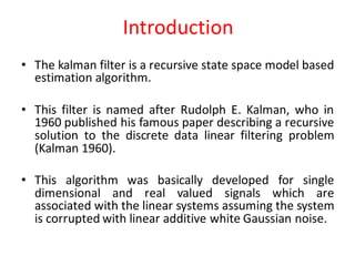
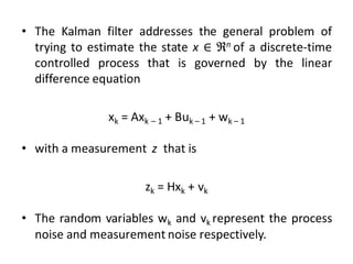
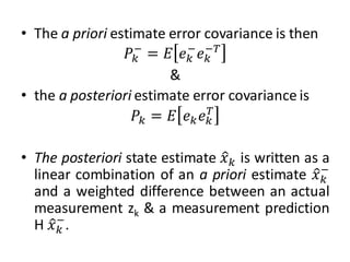
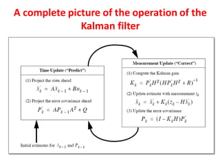
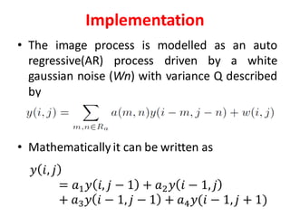
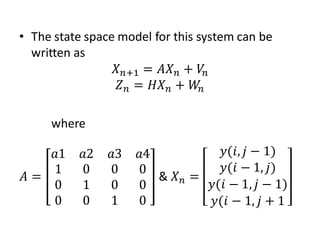
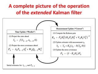
The document discusses the Kalman filter, an algorithm used to estimate the state of a linear dynamic system from a series of noisy measurements. It describes how the Kalman filter uses a predictor-corrector approach with time update and measurement update equations to estimate the true state. The filter is applied to image processing to reduce noise by modeling the image as an autoregressive process and using the Kalman filter estimates. Extensions to nonlinear and complex systems using the extended and complex Kalman filters are also covered.

1. KALMAN FILTER
Applications in Image processing

2. Introduction
• The kalman filter is a recursive state space model based
estimation algorithm.
• This filter is named after Rudolph E. Kalman, who in
1960 published his famous paper describing a recursive
solution to the discrete data linear filtering problem
(Kalman 1960).
• This algorithm was basically developed for single
dimensional and real valued signals which are
associated with the linear systems assuming the system
is corrupted with linear additive white Gaussian noise.

3. • The Kalman filter addresses the general problem of
trying to estimate the state x ∈ ℜn of a discrete-time
controlled process that is governed by the linear
difference equation
xk = Axk – 1 + Buk – 1 + wk – 1
• with a measurement z that is
zk = Hxk + vk
• The random variables wk and vk represent the process
noise and measurement noise respectively.

4. • The nxn matrix A in the previous difference
equation relates the state at the previous time
step k-1 to the state at the current step k , in the
absence of either a driving function or process
noise.
• The nxl matrix B relates the optional control input
u to the state x.
• The mxn matrix H in the measurement equation
relates the state to the measurement zk.

5. The Computational Origins of the Filter :
• We define𝑥 − ∈ℜn to be our a priori state
𝑘
estimate at step k given knowledge of the
process prior to step k , and 𝑥 𝑘 ∈ℜn to be our a
posteriori state estimate at step k given
measurement zk.
• We can then define a priori and a posteriori
estimate errors as
− −
𝑒𝑘 ≡ 𝑥𝑘 − 𝑥𝑘 &
𝑒𝑘 ≡ 𝑥𝑘 − 𝑥𝑘

6. • The a priori estimate error covariance is then
− − −𝑇
𝑃𝑘 = 𝐸 𝑒 𝑘 𝑒 𝑘
&
• the a posteriori estimate error covariance is
𝑇
𝑃𝑘 = 𝐸 𝑒 𝑘 𝑒 𝑘
• The posteriori state estimate 𝑥 𝑘 is written as a
linear combination of an a priori estimate 𝑥 − 𝑘
and a weighted difference between an actual
measurement zk & a measurement prediction
H 𝑥 −.
𝑘

7. .
𝑥 𝑘 = 𝑥 − + 𝐾 𝑧 𝑘 − 𝐻𝑥 −
𝑘 𝑘
• The difference 𝑧 𝑘 − 𝐻𝑥 −
𝑘 is called the
measurement innovation, or the residual.
• The nxm matrix K is chosen to be the gain or
blending factor that minimizes the a posteriori
error covariance.
• Substituting 𝑥 𝑘 in 𝑒 𝑘 and 𝑒 𝑘 in Pk , and
performing minimization, we get
𝑃− 𝐻 𝑇
𝑘
𝐾𝑘 = = 𝑃− 𝐻 𝑇 𝐻𝑃− 𝐻 𝑇 + 𝑅 −1
𝑘 𝑘
𝐻𝑃− 𝐻 𝑇 + 𝑅
𝑘

8. Kalman filter algorithm
• The Kalman filter estimates a process by using a form of
feedback control: the filter estimates the process state at
some time and then obtains feedback in the form of (noisy)
measurements.
• As such, the equations for the Kalman filter fall into two
groups: time update equations and measurement update
equations.
• The time update equations are responsible for projecting
forward (in time) the current state and error covariance
estimates to obtain the a priori estimates for the next time
step.

9. • The measurement update equations are responsible
for the feedback—i.e. for incorporating a new
measurement into the a priori estimate to obtain an
improved a posteriori estimate.
• The time update equations can also be thought of as
predictor equations, while the measurement update
equations can be thought of as corrector equations.
• The final estimation algorithm resembles that of a
predictor-corrector algorithm.

11. Discrete Kalman filter time update equations:
𝑥 − = 𝐴𝑥 𝑘−1 + 𝐵𝑢 𝑘−1
𝑘
Prediction
𝑃 − = 𝐴𝑃 𝑘−1 𝐴 𝑇 + 𝑄
𝑘
Discrete Kalman filter measurement update
equations:
𝐾 𝑘 = 𝑃 − 𝐻 𝑇 𝐻𝑃− 𝐻 𝑇 + 𝑅
𝑘 𝑘
−1
𝑥 𝑘 = 𝑥 − + 𝐾 𝑘 𝑧 𝑘 − 𝐻𝑥 −
𝑘 𝑘 Correction
𝑃 𝑘 = 𝐼 − 𝐾 𝑘 𝐻 𝑃−
𝑘

12. A complete picture of the operation of the
Kalman filter

13. Implementation
• The image process is modelled as an auto
regressive(AR) process driven by a white
gaussian noise (Wn) with variance Q described
by
• Mathematically it can be written as
𝑦 𝑖, 𝑗
= 𝑎1 𝑦 𝑖, 𝑗 − 1 + 𝑎2 𝑦 𝑖 − 1, 𝑗
+ 𝑎3 𝑦 𝑖 − 1, 𝑗 − 1 + 𝑎4 𝑦(𝑖 − 1, 𝑗 + 1)

14. • The state space model for this system can be
written as
𝑋 𝑛+1 = 𝐴𝑋 𝑛 + 𝑉𝑛
𝑍 𝑛 = 𝐻𝑋 𝑛 + 𝑊𝑛
where
𝑎1 𝑎2 𝑎3 𝑎4 𝑦(𝑖, 𝑗 − 1)
1 0 0 0 𝑦(𝑖 − 1, 𝑗)
𝐴= & 𝑋𝑛 =
0 1 0 0 𝑦(𝑖 − 1, 𝑗 − 1)
0 0 1 0 𝑦(𝑖 − 1, 𝑗 + 1

15. Results
Original Images Measured Images Corrected Images

16. Extended Kalman Filter
• An extended Kalman filter is used if the
process to be estimated and (or) the
measurement relationship to the process is
non-linear.
• Here
𝑥 𝑘 = 𝑓 𝑥 𝑘−1 , 𝑢 𝑘−1 , 𝑤 𝑘−1
• with measurement z that is
𝑧 𝑘 = ℎ 𝑥 𝑘, 𝑣 𝑘

17. • Similar to the Kalman filter, the time and
measurement equations for EKF can be
written as below:
• EKF time update equations:
• EKF measurement update eqns:

19. A complete picture of the operation
of the extended Kalman filter

20. Results
Original Image Measured Image Corrected Image

21. COMPLEX KALMAN FILTERING
• In complex Kalman filtering, image model is
represented in complex form as real and imaginary
values represented as real and imaginary part of the
complex number.
Y= Real+(imag)i
• where, Y is complex image model.
• Complex valued Kalman filters have been used
extensively in a variety of applications, including
frequency estimation of time-varying signals, training
of neural networks etc.

22. Properties of Kalman filter
• Kalman filter is a time-varying filter as Kalman gain
changes with n.
• The filter is very powerful in several aspects: it
supports estimations of past, present, and even
future states, and it can do so even when the precise
nature of the modeled system is unknown.
• In the Kalman filter, prediction acts like the prior
information about the state at time n before we
observe the data at time n.

23. Refernces
• Natasha Devroye. Estimation: parts of Chapters 12-13,
Wiener and Kalman Filtering.
• Greg Welch and Gary Bishop. An Introduction to the
Kalman Filter, Monday, July 24, 2006.
• R. E. KALMAN. A New Approach to Linear Filtering and
Prediction Problems.
• http://www.cs.unc.edu/~welch/kalman/