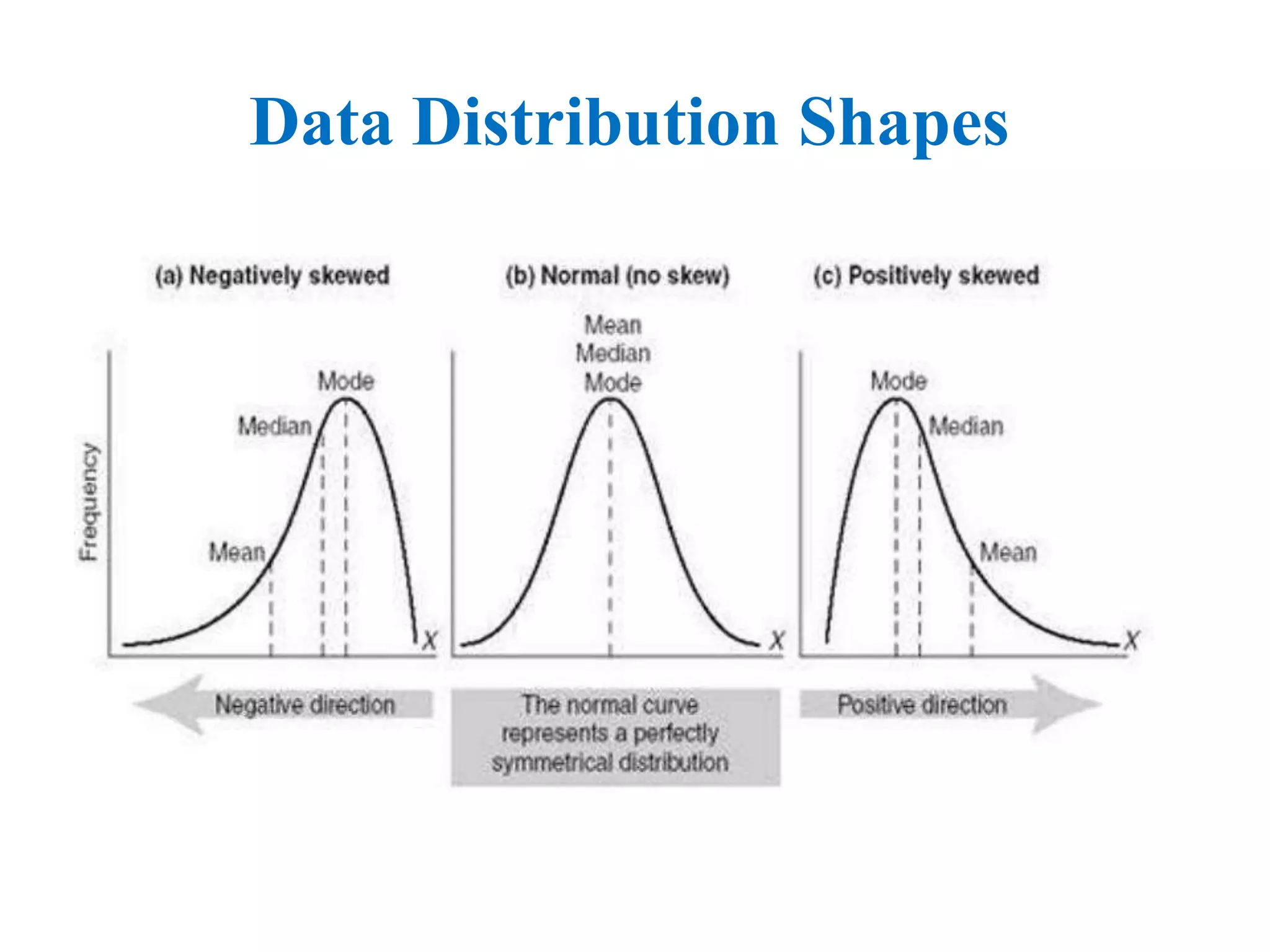
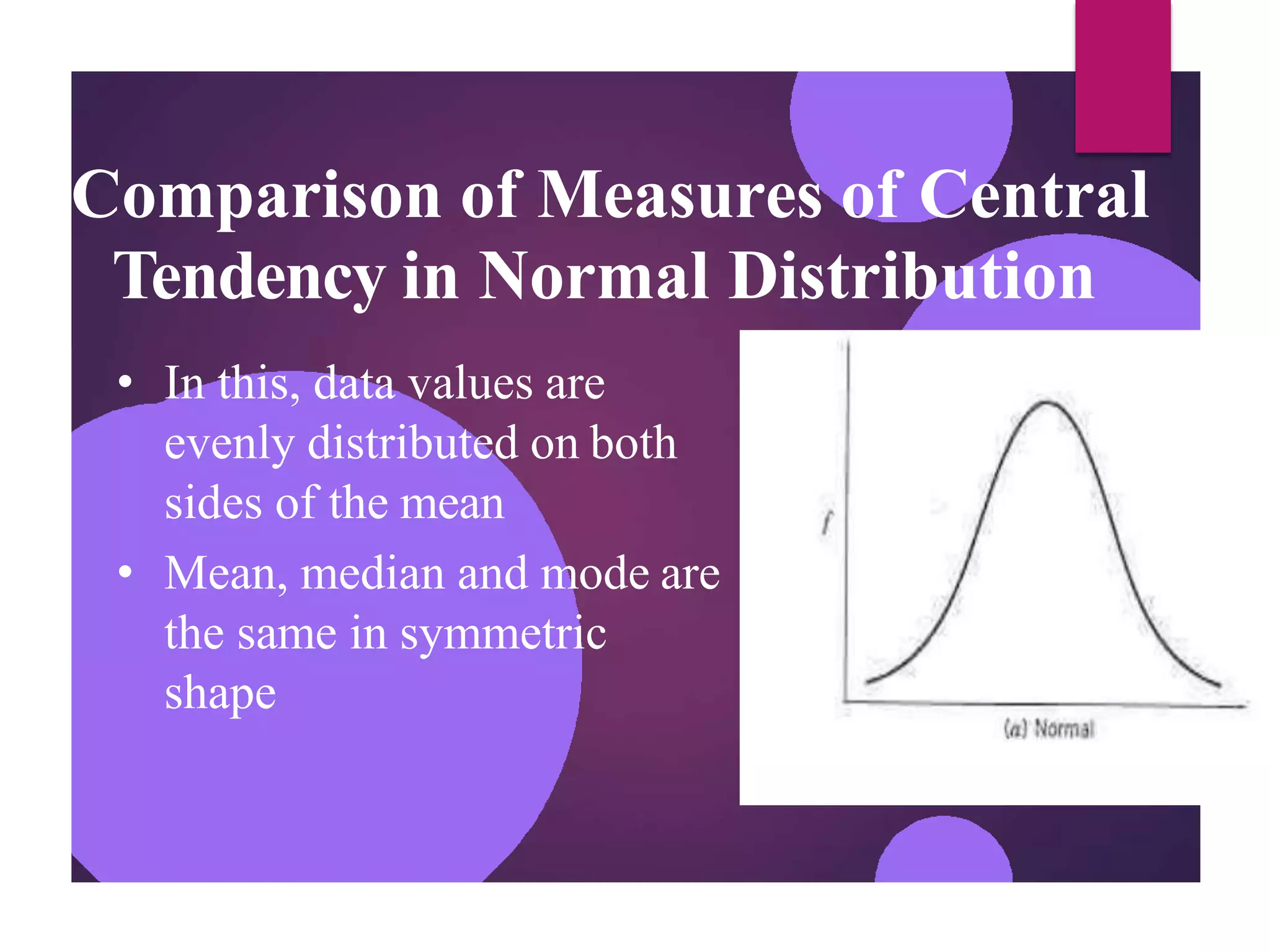
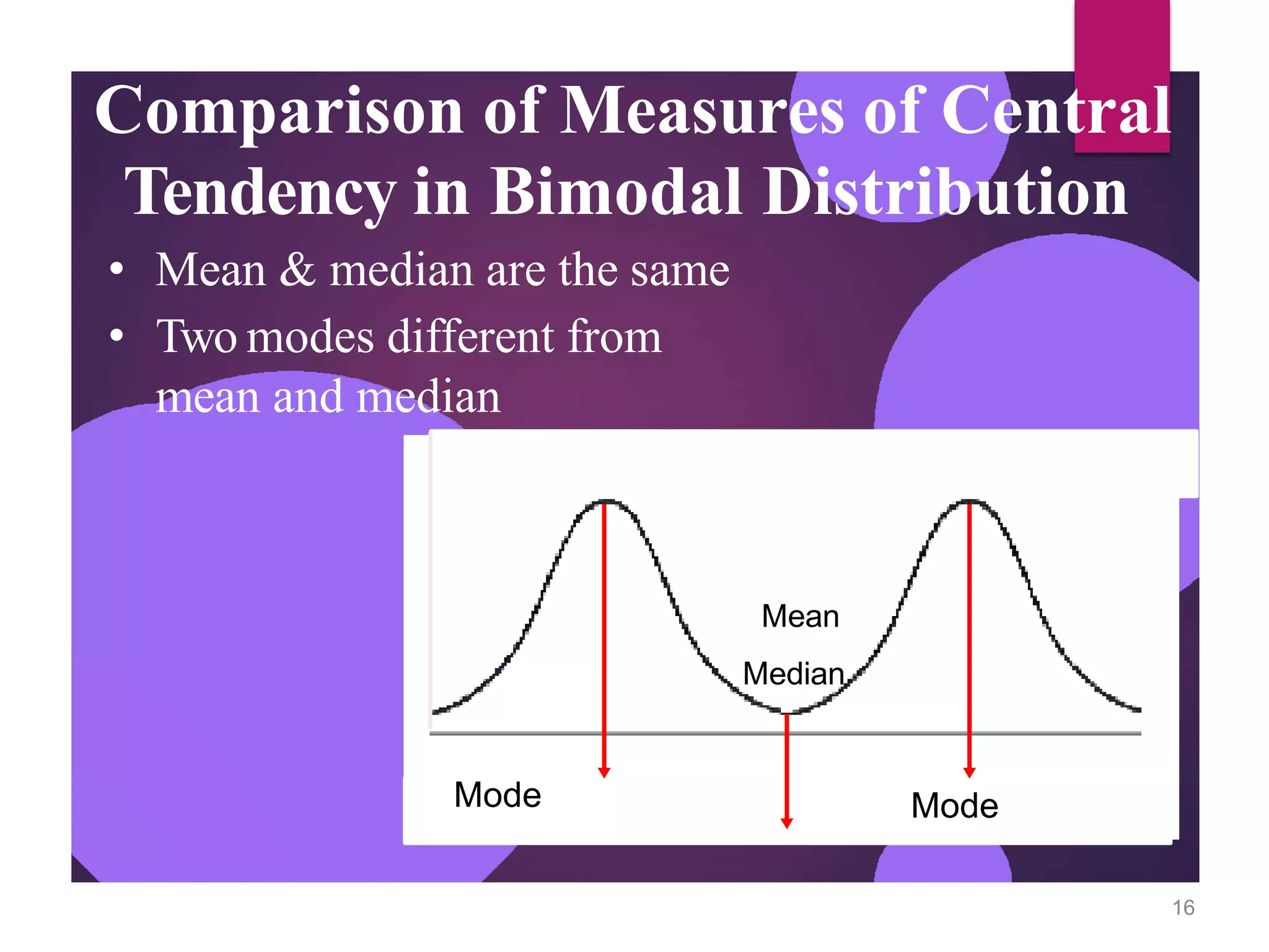
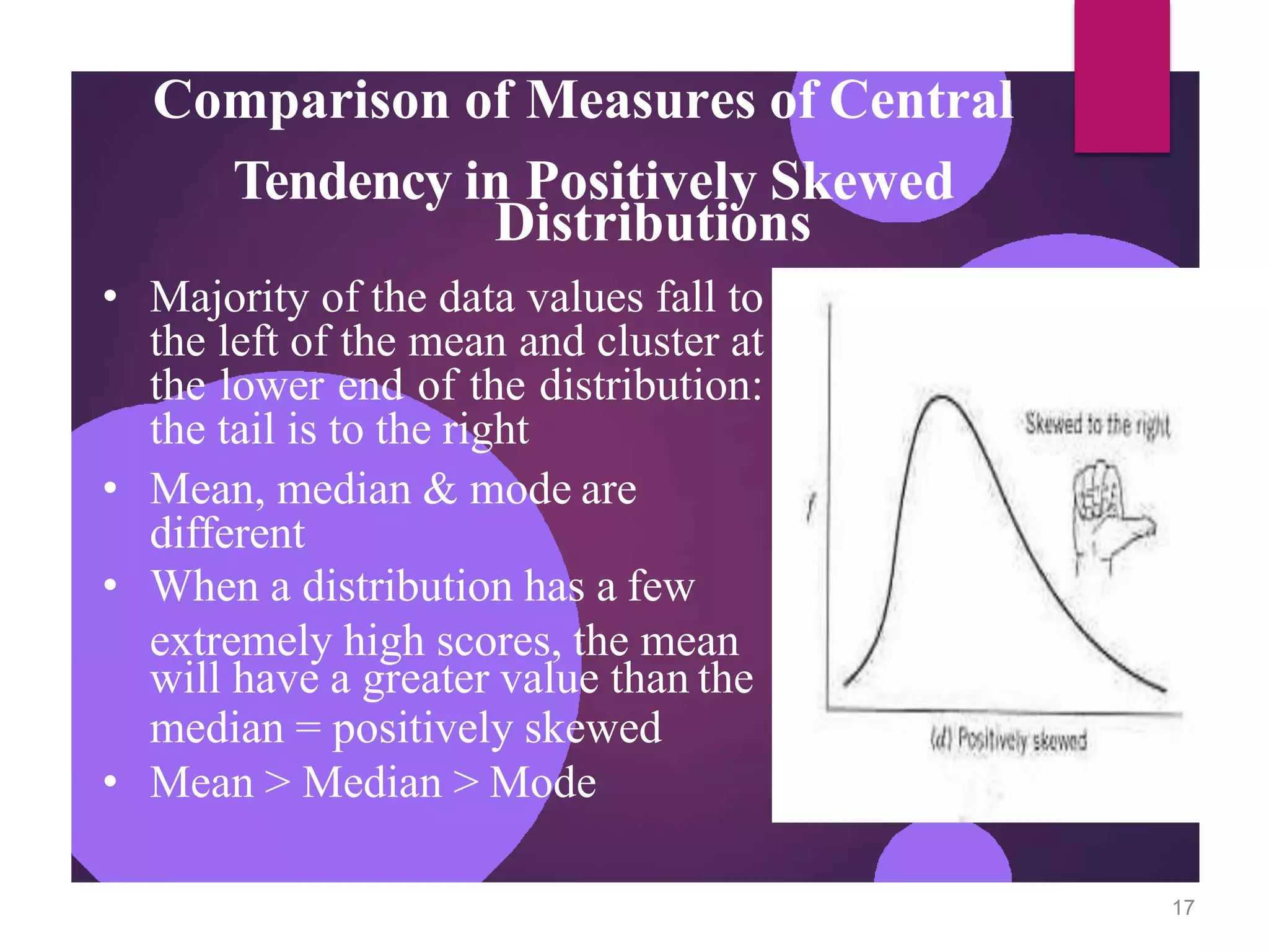
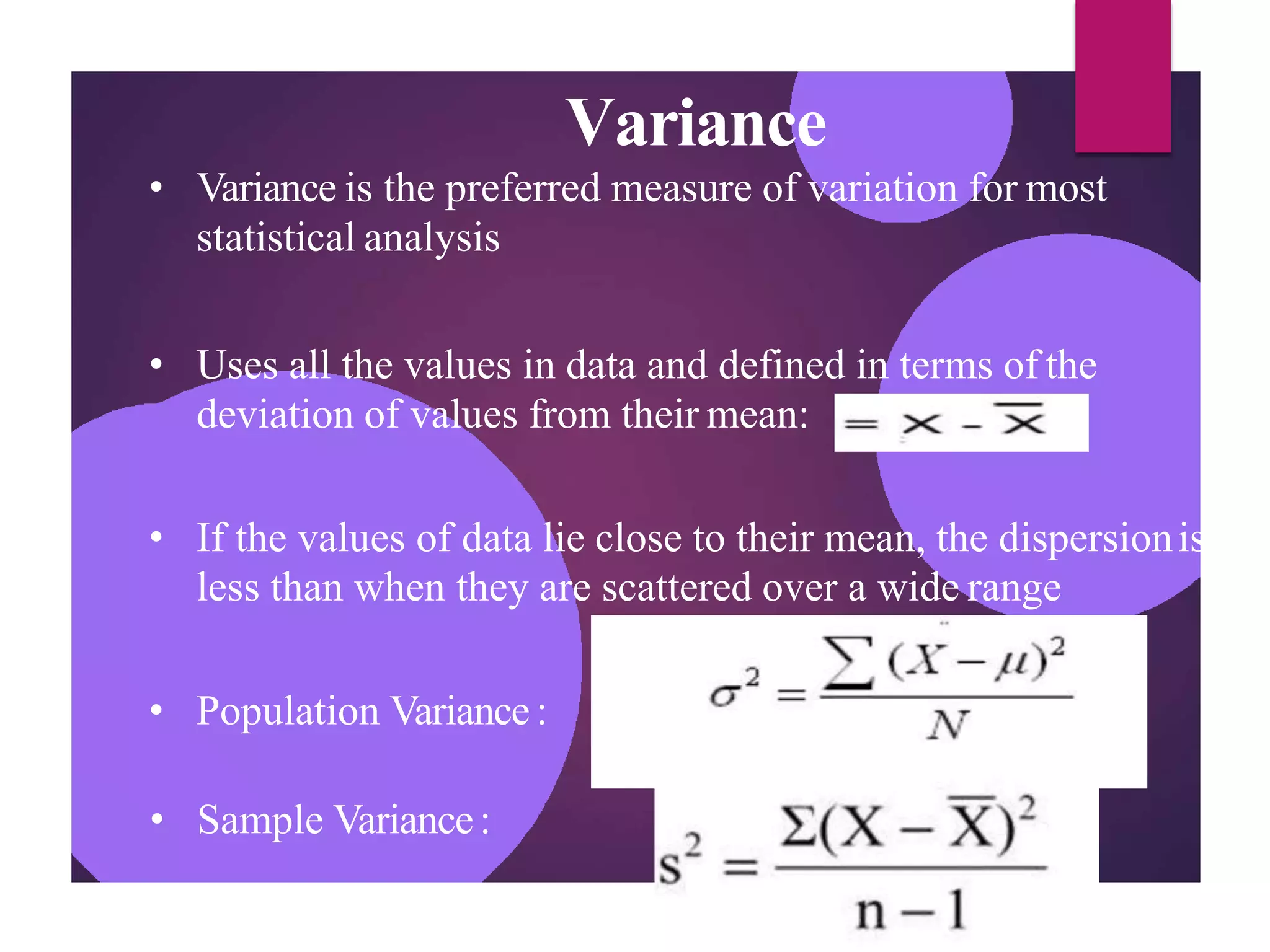
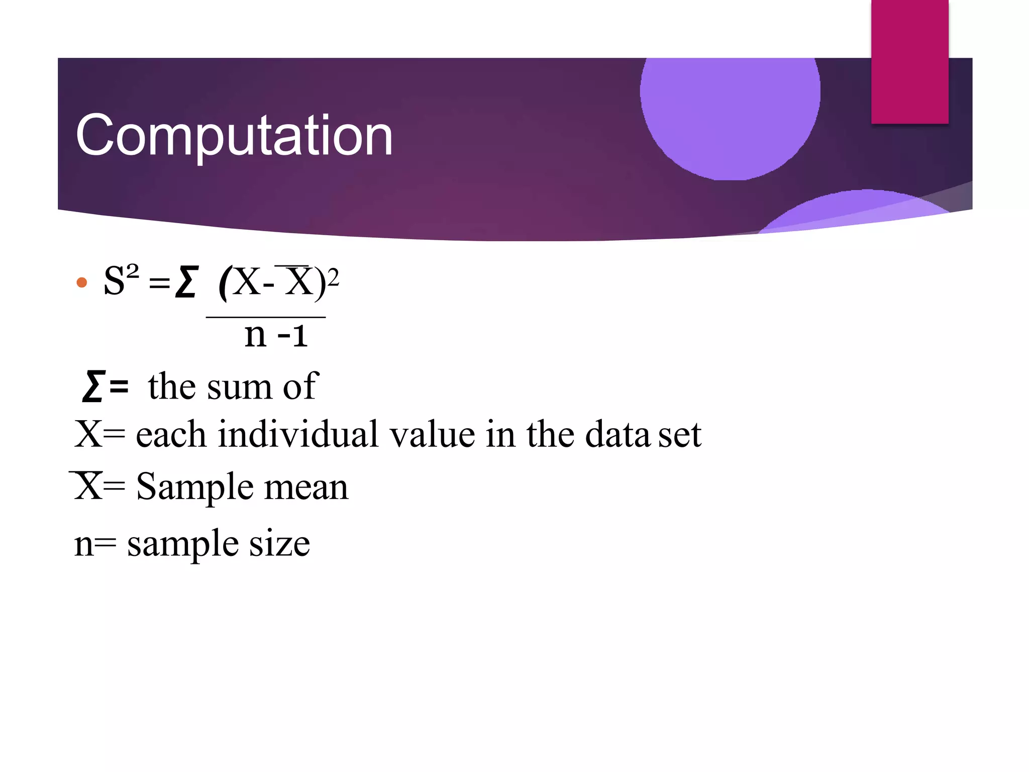
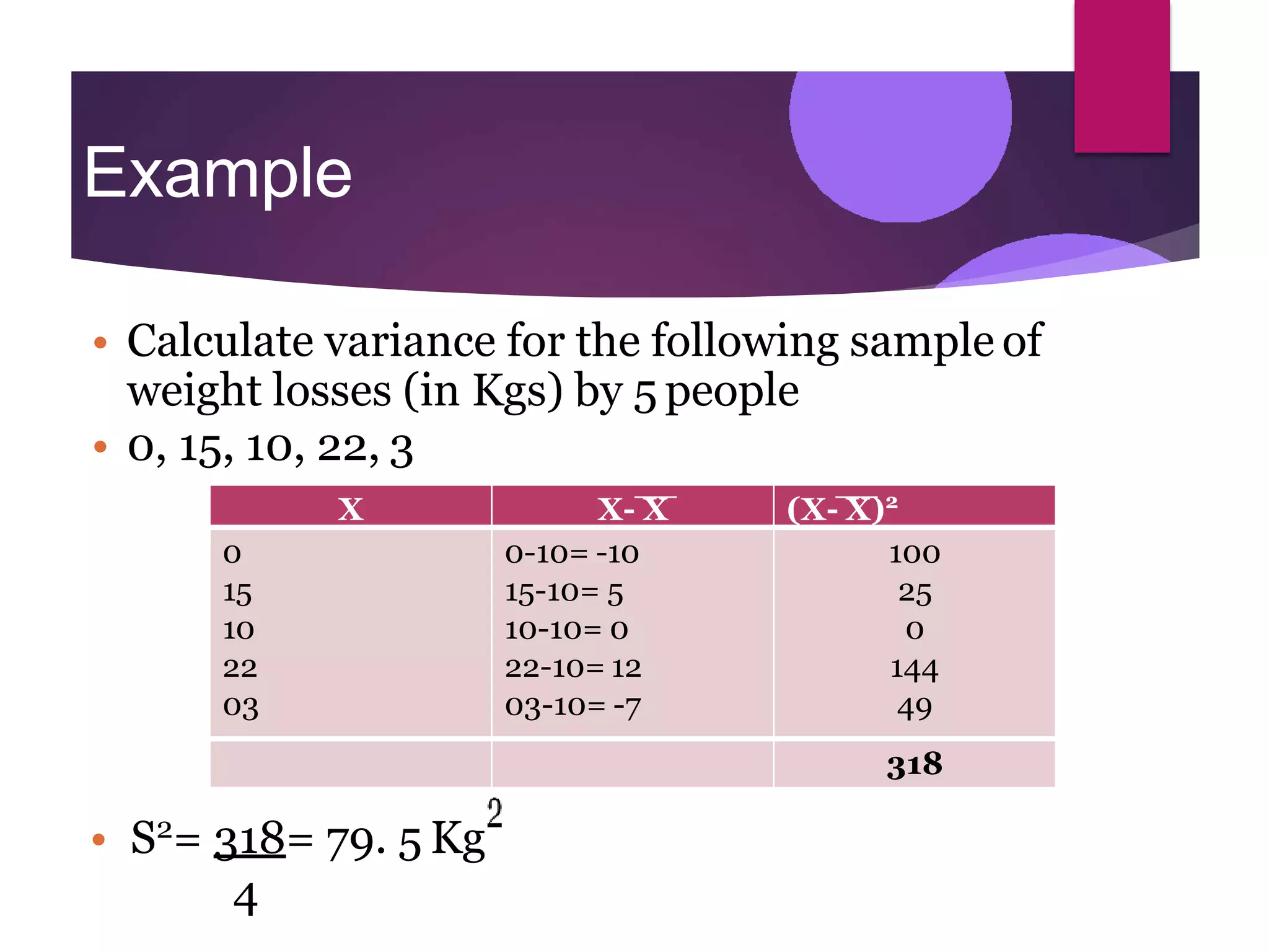
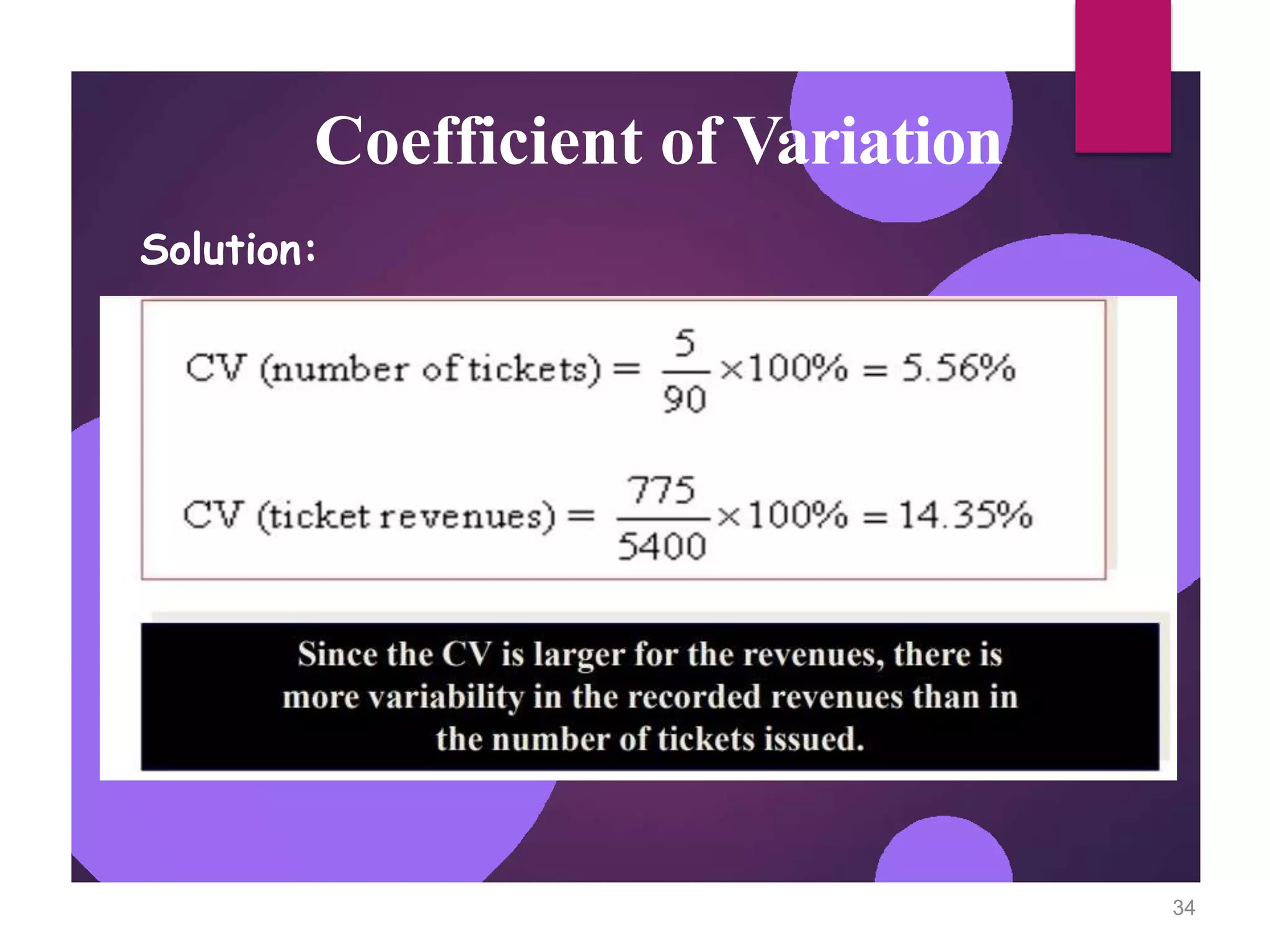
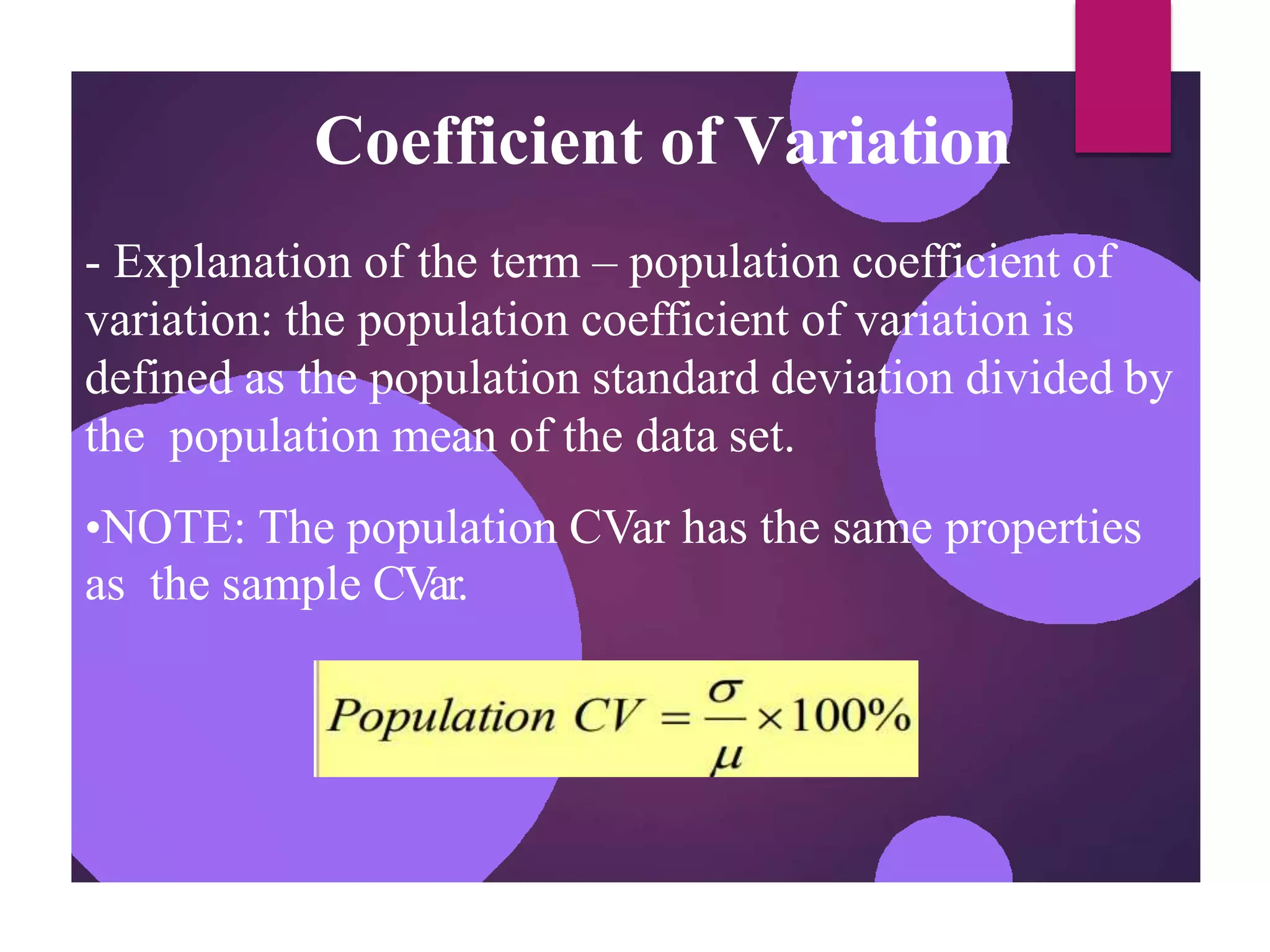
The document discusses measures of central tendency (mean, median, mode) and dispersion (variance, standard deviation) in statistical analysis, detailing their definitions, computations, and applications. It emphasizes the importance of these measures in summarizing data, identifying typical values, and understanding data variability. Additionally, the document provides examples and comparisons of different measures in various data distributions.

2. Measures of Central
Tendency and Dispersion
Shakir Rahman
BScN, MScN, MSc Applied Psychology, PhD Nursing (Candidate)
University of Minnesota USA.
Principal & Assistant Professor
Ayub International College of Nursing & AHS Peshawar
Visiting Faculty
Swabi College of Nursing & Health Sciences Swabi
Nowshera College of Nursing & Health Sciences Nowshera

3. Objective
s
• Define measures of central tendency
(mean, median, and mode)
• Define measures of dispersion (variance
and standard deviation).
• Compute the measures of central tendency
and Dispersion.
• Learn the application of mean and standard
deviation using Empirical rule and
Tchebyshev’s theorem

4. Lets answer a few
questions!
• What is the age of year 3 BScN students, class of
2020?
• How many hours per week, do BScN year 3
students spend on studying biostatistics?
• What is the height of boys enrolled in BScN
program at AICNAHS?

5. Measures of Central
Tendency
• A measure of the central tendency is a
value about which the observations tend to
cluster.
• In other words it is a value around which a
data set is centered.
• The three most common measures of central
tendency are mean, median and mode.
(Munro; Bluman, 2001)

6. Why is it
needed?
• To summarize the data.
• It provides with a typical value that gives the
picture of the entire data set
(Bluman, 2004)

7. Mean
It is the arithmetic average of a set of numbers, It is the
most common measure of central tendency.
Computed by summing all values in the data set and
dividing the sum by the number of values in the data set
Properties
• Applicable for interval and ratio data
• Not applicable for nominal or ordinal data
• Affected by each value in the data set, including
extreme values.

8. Formula
• Mean is calculated by adding all values in the data
set and dividing the sum by the number of values in
the data set.
• X- = X1 + X2 + X3 +. . . . . .Xn
n
∑= the sum of
X= each individual value in the data set
n= sample size (Sample)
N = sample size (Population)

9. Sample Mean:
Age of the patients coming to the clinic
57,86,42,38,90,66
X  X
 X1  X2  X3 ... Xn
n n
 57 86 4238 9066
6
 379
6
 63.167

10. Practice
time!
•The salaries of five faculty members working at
AICNAHS are:
20,000, 18,000 24,000 30,000 22,000
Calculate the mean salary of the faculty members

11. • X= 20,000+ 18,000+ 24,000+ 30,000+22,000
5
X = 114000
5
X= 22,800

12. Properties of
mean
• Affected by the extreme high and low values in
the data set
• 5, 6, 5, 8, 8, 7
• 5, 6, 5, 4, 20, 18
• 13,10, 11, 10, 0, 1
• Therefore, it works best for symmetrical
frequency distributions.
(Bluman, 2004)

13. Median
• Mid-point or Middle value of the data when the
measurements are arranged in ascending order.
• A point that divides the data into two equalparts
Median: Computational Procedure
• Arrange the observations in an ascending order.
• If there is an odd number of terms, the median is the
middle value and If there is an even number of
terms, the median is the average of the middle two
terms
(Bluman, 2004)

14. Properties of Median
• Applicable for ordinal, interval, and ratio data
• Not applicable for nominal data
• Very simple and easy to calculate
• Unaffected by extremely large and extremely
small values.
• It is used when one must determine whether
the data values fall into the upper half or lower
half of the distribution

15. Median Example (with an Odd
Number) Arranged data in ascending order
14, 16, 21, 27, 27, 39, 45
• Position of median = (n+1)/2 = (7+1)/2 = 4
• There are 7 terms in the ordered array.
• The median is the 4th term, 27 years.
• If the 45 is replaced by 100, the median is 27 years.
• If the 14 is replaced by -103, the median is 27 years.

16. Median Example(with an Even Number)
Arranged data in ascending order
12, 14, 16, 21, 27, 27, 39, 45
• There are 8 terms in the ordered array.
• Position of median = (n+1)/2 = (8+1)/2 = 4.5
• The median is between the 4th and 5th terms,
(21+27)/2 = 24 years
• If the 16 is replaced by 100, the median is 24years.
• If the 12 is replaced by -88, the median is 24years

17. Practice
• Following are the number of family members in
selected houses in two communities. Calculate
median:
• 17, 4, 15, 12, 18
• Arrange in ascending order
• Since there are 5 values there fore, (5+1)= 3
2
• Third number in the data set, after arrangement
in ascending order, is the median

18. Contd
…
• 17, 4, 15, 12, 18, 11
• Since there are 6 values there fore, (6+1)= 3.5
2
• This means that the median is between the 3rd
and the 4th term
• So mean of 12 and 15 will be the median for this
data set

19. Contd
…
• Following are the values of pain intensity of 8
patients admitted with angina. These have been
marked by the patients on a scale of 0-10.
Calculate median:
• 9, 7, 4, 10, 3

20. Properties of
Median
14, 15, 23, 28, 30
• Not sensitive to extreme values; can be used for
skewed data
• If 30 is replaced by 100, in the above example,
still the median remains 23.
• If 14 is replaced by 2, in the above example, still
the median remains 23.

21. Mode
• The mode is the observation that occurs most
frequently in the data set.
• There can be more than one mode for a data set
OR there maybe no mode in a data set.
• Is also applicable to the nominal data

22. Practice
• Calculate mode for the following data set of :
▫ Sale of different brands of shampoo in a week
(Pantene= 1, head & shoulders=2, sun silk= 3) :
• 1, 1, 2, 3, 2, 3, 2, 1, 2, 2, 2, 1, 3
▫ Pain scores of 5 patients
• 6, 4, 2, 10, 7
▫ Scores of biostats exam
• 75, 80, 92, 42, 80, 68, 75

23. Mode Example: Nominal Data

24. Frequency
Mode Example: Discrete variable
50
45
40
35
30
25
20
15
10
5
0
1 2 3 4 5 6 7 8 9 10 11 12 13 14 15 16 17 18 19 20 21 22 23
Number of golf clubs 13

25. Data Distribution Shapes

26. Comparison of Measures of Central
Tendency in Normal Distribution
• In this, data values are
evenly distributed on both
sides of the mean
• Mean, median and mode are
the same in symmetric
shape
1

27. Comparison of Measures of Central
Tendency in Bimodal Distribution
• Mean & median are the same
• Two modes different from
mean and median
16
Mean
Median
Mode Mode

28. Comparison of Measures of Central
Tendency in Positively Skewed
17
Distributions
• Majority of the data values fall to
the left of the mean and cluster at
the lower end of the distribution:
the tail is to the right
• Mean, median & mode are
different
• When a distribution has a few
extremely high scores, the mean
will have a greater value than the
median = positively skewed
• Mean > Median > Mode

29. Comparison of Measures of Central
Tendency in Negatively Skewed
Distributions
Majority of the data values fall to
the right of the mean and cluster
at the upper end of the
distribution: the tail is to the left
Mean, median & mode are
different
When a distribution has a few
extremely low scores, the mean
will have a lower value than the
median = negatively skewed
• Mode > Median > Mean

30. Mean
Median
No Mode

31. No
(so
Lev
inal, Ordinal, and
metimes) Interval/Ratio-
el Data
Interval/Ratio-Level Data
Comparison of Measures of Central
T
endency
Mode
Most frequently occurring value
Nominal, Ordinal, and
(sometimes) Interval/Ratio-
Level Data
Ordinal-Level Data and
Interval/Ratio-Level data
(particularly when skewed)
Median
Exact center (when odd N) of
rank-ordered data or average of
two middle values.
Mean
Arithmetic average
(Sum of Xs/n)

32. Use of measures of central tendency
• Mean is the most common measure which uses
each value in the data set. It is best to be used
when the distribution is symmetrical
• If the distribution is skewed, then median is a
better measure of central tendency as it is
unaffected by the extreme values
• Mode depicts the most preferred or the most
popular product, candidate etc. Can be
calculated for all levels of data but is not very
meaningful for interval and ratio scale data

33. Recap

34. Measures of Dispersion

35. Measures of
Dispersion
• Calculate mean for the following data sets:
• 5, 6, 8, 10, 12, 14, 15
• 1, 4, 8, 10, 12, 16, 19
• Then what’s the difference between the following
data sets?
• The difference is in the spread of both data sets;
the spread of the second data set is more than
the first one
(Bluman, 2004)

36. Why is it important to know the
dispersion of data?
• Example:
• Scores of student A: 23, 32, 74, 56, 48
• Scores of student B: 55, 67, 63, 57, 65
• Ages of sample 1: 12, 15, 22, 34, 50,56
• Ages of sample 2: 10, 12, 14, 18, 17,16
• It shows the consistency and
homogeneity/heterogenity in the data

37. Measures of Variability
• Measures of variability describe the spread or the
dispersion of a set of data.
• If all the values in a data set are same there is no
dispersion BUT dispersion is present when values are
not same in data set.
• The amount of dispersion may be small, when the
values though different are close together
Common Measures of
Variability:
 V
ariance
 Standard Deviation
– Range
–Coefficient of
Variation

38. Range
•The difference between the largest and the smallest
values in a set of data
• Simple to compute
• Ignores all data points except the two
extremes.
Example:
Range = Largest – Smallest
= 48 - 35 = 13
The range is quick to compute but fails to be very
useful since it considers only the extreme values and
does not take into consideration the bulk of the
observations. It is not widely used.

39. Variance
• Variance is the preferred measure of variation for most
statistical analysis
• Uses all the values in data and defined in terms of the
deviation of values from their mean:
• If the values of data lie close to their mean, the dispersionis
less than when they are scattered over a wide range
• Population Variance:
• Sample Variance:

41. Computation
• S2
=∑ (X- X)2
n -1
∑= the sum of
X= each individual value in the data set
X= Sample mean
n= sample size

42. Example
• Calculate variance for the following sample of
weight losses (in Kgs) by 5 people
• 0, 15, 10, 22, 3
• S2
= 318= 79. 5 Kg
4
X X- X (X- X)2
0
15
10
22
03
0-10= -10
15-10= 5
10-10= 0
22-10= 12
03-10= -7
100
25
0
144
49
318

43. Sample Variance
Average Systolic Blood Pressure of the values from the 6 Cardio
patients are: 130, 138, 188, 188, 112, 162, and 160.
Arithmetic mean (=148.3 mmHg)

44. Standard Deviation
• Standard Deviation is defined as the square root of the
variance
• It is more convenient to express the variation in the
original units by taking the square root of the variance
• Population Standard Deviation
• Sample Standard Deviation:

45. Standard Deviation
• It is the square root of variance
•Population standard deviation is denoted by σ
•Sample standard deviation is denoted by s
• S= √S2
(Bluman, 2004)

46. Sample Standard
deviation
- Average distance of the values from thearithmetic
mean - Square root of the sample variance
Where Mean is
27years
S = 794 = 132.33
6
S2
=√S = √132.33yrs
S = 11.5 yrs

47. Mean & Standard deviation for Grouped
data
When data is presented in grouped form, the mean
and variance are computed by following equations:
Where “fi” is the number of observations in the
respective class interval and c is the number of
classes.

49. The Variance and Standard
Deviation
When the data are clustered about the mean, the
variance and standard deviation will be somewhat
small.

50. The Variance and Standard
Deviation
When the data are widely scattered about the mean, the
variance and standard deviation will be somewhat large.
28

51. Coefficient of Variation
• When two data sets have the same unit, their
standard deviations can be compared directly.For
e.g. we can compare the standard deviations ofthe
mileage of two brands of cars. If in a particular year,
the standard deviation of the mileage of Mehran is
360 miles and of Vitz is 200 miles, then we can say
that there is more variation in the mileage of
mehran than Vitz.
• It was possible to compare the two SDs because
their units were same

52. Contd..
.
• But if we want to compare the SD of two variables
whose units are different then what?
• For instance, a manager wants to compare the SD of
number of sales done by salesmen per year to the SD
of commission made by these salespersons
• In such cases Coefficient of Variation is calculated
(Bluman, 2004)

53. Coefficient of Variation
One important application of the mean and the standard
deviation is the coefficient of variation.
CVar= Standard Deviation x 100
Mean
The coefficient of variation depicts the size of the standard
deviation relative to its mean. Since both standard deviation and
the mean represent the same units the units cancel out and the
coefficient of variation becomes a pure number.

54. Coefficient of Variation
The CV is useful for comparing scatter of variables
measured in different units
Examples:
The mean number of parking tickets issued in a
neighborhood over a four-month period was 90, and
the standard deviation was 5.
The average revenue generated from the tickets was
$5,400, and the standard deviation was $775.
Compare the variations of the two variables.

55. Coefficient of Variation
Solution:
34

56. Coefficient of Variation
- Explanation of the term – population coefficient of
variation: the population coefficient of variation is
defined as the population standard deviation divided by
the population mean of the data set.
•NOTE: The population CVar has the same properties
as the sample CVar.

57. References
• Bluman, A. (2004). Elementary statistics: A
step by step approach. Boston: Mc Graw Hill.

58. Acknowledgments
Dr Tazeen Saeed Ali
RM, RM, BScN, MSc ( Epidemiology & Biostatistics), Phd (Medical
Sciences), Post Doctorate (Health Policy & Planning)
Associate Dean School of Nursing & Midwifery
The Aga Khan University Karachi.
Kiran Ramzan Ali Lalani
BScN, MSc Epidemiology & Biostatistics
Aga Khan University Karachi