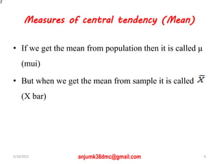
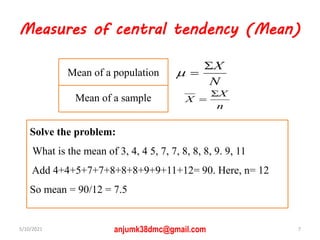
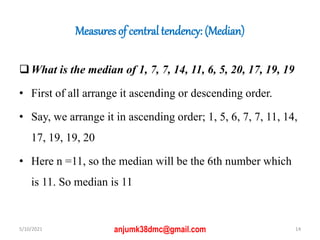
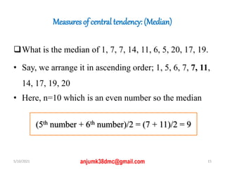
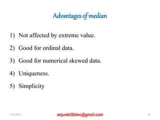
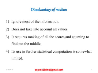
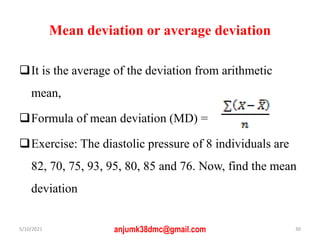
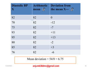
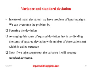
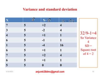
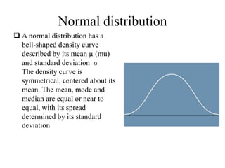
Central tendency and dispersion

Central Tendency and Dispersion
Prof Md Anisur Rahman
MBBS, DO, FCPS (eye)
Head of the department
(Ophthalmology) DMC
5/10/2021 1
anjumk38dmc@gmail.com

. Characteristic of central tendency
 Central tendency of a data set is the tendency of data to cluster
around a central point of the series.
 Measures of central tendency is a single typical value of a data
set that represent a set of data and around which other values
of data set are found to cluster.
 To get a single value, that represents the entire data &
describes the characteristic of whole set of data.
5/10/2021 2

What are the central tendencies?
1. Mean
2. Median
To some extent
3. Mode
5/10/2021 3

Measures of central tendency: (Mean)
1) What is mean?
2) Advantages of mean
3) Disadvantages of mean
4) Formula to calculate the mean
5) Solve the problem
5/10/2021 anjumk38dmc@gmail.com 4

What is Mean?
Mean is the sum of scores divided by the total
number of Observations. It is commonly used in
statistics.
Sometimes mean is denoted by µ (mui) and sometimes
by (X bar)
BUT WHY?
5/10/2021 5

Measures of central tendency (Mean)
• If we get the mean from population then it is called µ
(mui)
• But when we get the mean from sample it is called
(X bar)
5/10/2021 6

Measures of central tendency (Mean)
n
X
X


N
X



Mean of a sample
Mean of a population
Solve the problem:
What is the mean of 3, 4, 4 5, 7, 7, 8, 8, 8, 9. 9, 11
Add 4+4+5+7+7+8+8+8+9+9+11+12= 90. Here, n= 12
So mean = 90/12 = 7.5
5/10/2021 7

Advantages of mean
1. Uniqueness: only one mean for a set of data.
2. Simplicity: easy to calculate and understand.
3. Sensitivity: sensitive to and affected by all values,
that means it uses all the information in the
distribution.
5/10/2021 8

Advantages of mean
4. Can be applied in all normally distributed numerical
data.
5. Used as the basis of further most common and most
powerful statistical computation.
6. Means of sub-groups may be combined to get the
mean of entire group. (Unlike median & mode).

Disadvantages of mean
1) Grossly affected by extreme values (outliers) of
data.
2) Not useful in skewed distribution of data.
5/10/2021 10

Measures of central tendency: (Median)
1) When we use median?
2) How to calculate median?
3) Solve the problem
4) Advantages of median
5) Disadvantage of median
6) Why median is not enough?
5/10/2021 11

Have you ever think that, why some scientific article
use median, in spite of mean? Remember when the
data set is not in normal shaped, it is skewed in spite
of mean we use median.
5/10/2021 12

How to calculate median?
 Middle most value of data set arranged in ascending
or descending order.
 If odd number of values, middle most value is the
median
 If even number of values, mean of the middle two
values is the median.
5/10/2021 13

What is the median of 1, 7, 7, 14, 11, 6, 5, 20, 17, 19, 19
• First of all arrange it ascending or descending order.
• Say, we arrange it in ascending order; 1, 5, 6, 7, 7, 11, 14,
17, 19, 19, 20
• Here n =11, so the median will be the 6th number which
is 11. So median is 11
5/10/2021 14

What is the median of 1, 7, 7, 14, 11, 6, 5, 20, 17, 19.
• Say, we arrange it in ascending order; 1, 5, 6, 7, 7, 11,
14, 17, 19, 20
• Here, n=10 which is an even number so the median
5/10/2021 15
(5th number + 6th number)/2 = (7 + 11)/2 = 9

Advantages of median
1) Not affected by extreme value.
2) Good for ordinal data.
3) Good for numerical skewed data.
4) Uniqueness.
5) Simplicity
5/10/2021 16

Disadvantage of median
1) Ignore most of the information.
2) Does not take into account all values.
3) It requires ranking of all the scores and counting to
find out the middle.
4) Its use in further statistical computation is somewhat
limited.
5/10/2021 17

Why median is not enough?
The median is known as a measure of location; that
is, it tells us where the data are.
As stated in, we do not need to know all the exact
values to calculate the median; if we made the
smallest value even smaller or the largest value even
larger, it would not change the value of the median.
5/10/2021 18

Why median is not enough?
Thus the median does not use all the information in
the data and so it can be shown to be less efficient
than the mean or average, which does use all values
of the data.
5/10/2021 19

Measures of central tendency
(Mode)
1) What is mode?
2) Advantages of mode
3) Disadvantages of mode
4) Solve the problems

What is mode?
It is the most frequent and repeated values observed
in a data set.
It is the most common score in a frequency
distribution e.g. in a data set: 1, 2, 2, 2, 3, 4, 5, 6; the
mode is 2

Advantages of mode
1) Not affected by extreme values and the skewness of
data.
2) Simplicity.
3) Good for bimodal distribution.

Disadvantages of mode
1) Often not clear defined.
2) Not much used in statistics.
3) Ignore most of the information

Measures of Dispersion
In statistics, dispersion denotes how stretched or
squeezed a distribution is.
Dispersion is contrasted with location or central
tendency, and together they are the most used
properties of distributions.

Following are the measures of dispersion of individual
observation
1) Range
2) Interquartile range
3) Mean deviation
4) Variance
5) Standard deviation
6) Co-efficient of variation

Range (Variability)
The range is equal to the high score minus the low score
in a distribution
• Say in your study you take the age of 10 people.
• They are as follows 25, 48, 22, 34, 33, 34, 38, 40, 60, 29,
• What is the range?
• You arrange them in ascending or descending order

Range (Variability)
22,25,29,33,34,34,38,40,48,60.
So the range is (minimum 22, and maximum 60) = 60
– 22 = 38
Here only 10 data has taken so you can do it
manually. But when the data is large enough it is very
much tedious to calculate manually. We have to use
SPSS. Or EXCEL file.

Interquartile range
 Range is a measure based on two extreme observations and it
fails to take account of the scatter within the range. In
Interquartile range some extreme observations on two sides are
discarded.
• 1/4 = 25% of observations at the lower end and another ¼ =
25% of observations at the upper end and Interquartile range
include the middle 50% of observations
25% 25% 25% 25%

Interquartile range
Q1 Q2 Q3
50%
Interquartile range represents the difference between the
third quartile and first quartile. Symbolically, Interquartile
range = Q3―Q1

Mean deviation or average deviation
It is the average of the deviation from arithmetic
mean,
Formula of mean deviation (MD) =
Exercise: The diastolic pressure of 8 individuals are
82, 70, 75, 93, 95, 80, 85 and 76. Now, find the mean
deviation

Diastolic BP
X
Arithmetic
mean
Deviation from
the mean X―
82 82 0
70 82 -12
75 82 -7
93 82 +11
95 82 +13
80 82 -2
85 82 +3
76 82 -6
Mean deviation = 54/8 = 6.75

Variance and standard deviation
• In case of mean deviation we have problem of ignoring signs.
We can overcome the problem by-
 Squaring the deviation
 Averaging this sums of squared deviation that is by dividing
the sums of squared deviation with number of observations (n)
which is called variance
 Now if we take square root the variance it will become
standard deviation.

X X-
7 5 +2 4
3 5 -2 4
4 5 +1 1
6 5 -1 1
1 5 -4 16
6 5 +1 1
7 5 +2 4
6 5 +1 1
5 5 0 0
32/9-1=4
So Variance
4
SD =
Square root
of 4 = 2

• Variance is used most commonly with more advanced
statistical procedures such as regression analysis,
analysis of variance (ANOVA), and the determination
of the reliability of a test
• The variance is also known as the mean square
(MS)

To calculate the standard deviation follows the following
stages
1) First of all to calculate the arithmetic mean of all
deviations
2) Now to take the deviation of each value from the
arithmetic mean
3) Then square each deviation
4) To add up the squared deviation

5) To divide the result by the number of observations n
or n-1 (for population n, for sample size less than
30, n-1)
6) Then to take the square root, which gives the
standard deviation

Example OF SD
Consider two students, each of whom has taken
five exams.
• Student A has scores 84, 86, 83, 85, and 87.
• Student B has scores 90, 75, 94, 68, and 98.
• Compute the SD for both Student A and Student B

Here is the calculation for student A.
MARKS OF “A” MEAN DIFFERENCE SQUARE
84 85 -1 1
86 85 +1 1
83 85 -2 4
85 85 0 0
87 85 +2 4
10
10/5-1 1.58

Here is the calculation for student B.
MARKS OF “A” MEAN DIFFERENCE SQUARE
90 85 +5 25
75 85 -10 100
94 85 +9 81
68 85 -17 289
98 85 +13 169
664
664/5-1 12.88

• Since the standard deviation of Student B’s scores is greater
than that of Student A’s (12.88 > 1.58), Student B’s scores are
not as consistent as those of Student A.
• Standard deviation gives us an idea of the “spread” of
the dispersion; that the larger the Standard deviation, the
greater the dispersion of values about the mean.

Exercise: 1
Average weight of baby at birth is 3.05 kg with the
SD of 0.39 kg. If the birth is normally distributed
would you regard as weight of 4 kg is abnormal? And
weight of 2.5 kg is normal?

Solution:
Normal limits of weight at ± 1.96 SD (3.05 ± 1.96 x
0.39) will be 2.29 kg and 3.81 kg. The weight of 4 kg
falls outside the normal limits (since 4> 3.81) so it is
taken as abnormal.
The weight of 2.5 kg lies within the normal limits of
2.29 and 3.81 so it is not taken as abnormal.

coefficient of variation (CV)
• The coefficient of variation is a measure of spread
that describes the amount of variability relative to the
mean. Because the coefficient of variation is unit less,
we can use it instead of the standard deviation to
compare the spread of data sets that have different
units or different means.

EXAMPLE: Co-efficient of variation
In a series of 40 adults, mean systolic blood pressure
was 120 and SD was 10. In another series of 30 adults
mean height and SD were 160 cm and 5 respectively.
Now find which character show greater variation.

We Know
CV of BP = (10/120) X 100 = 8.33%
CV of Height = (5/160) X100 = 3.13%
Thus BP is found to be a more variable character
than height (8.33/3.13) = 2.66 times

The list below shows the symbols used in certain
statistical measures
𝐱 = the sample mean- note the bar over the X. We can say 'the
mean of X' or just 'X bar' when reading this.
• μ = the population mean (pronounced mew)
• S2 = the sample variance (say S squared)
• ἀ2 = the population variance (pronounced sigma)
• S = the sample standard deviation
• σ = the population standard deviation (sigma)

Population statistics are referred to using
Greek symbols and
sample statistics use letter from the Roman
alphabet.

 There are several types of data distribution in statistics.
 Normal distribution
 Binomial distribution
 Poisson distribution
 And many other types.
• Among them all, Normal distribution of data is widely used

Normal distribution
 A normal distribution has a
bell-shaped density curve
described by its mean µ (mu)
and standard deviation σ
The density curve is
symmetrical, centered about its
mean. The mean, mode and
median are equal or near to
equal, with its spread
determined by its standard
deviation

Binomial distribution model
It is an important probability model that is used when
there are two possible outcomes (hence "binomial").Each
replication of the process results in one of two possible
outcome (success or failure), The probability of success is
the same for each replication, and the replications are
independent, meaning here that a success in one patient
does not influence the probability of success in another.

The Normal Distribution. Why it is important?
 It is very important to test data whether data is normally
distributed or not, because statistical test depends upon the
data distribution.
 If data is normally distributed then parametric test will be
done.
 If data is not normally distributing then non-parametric test
 Parametric tests are more powerful than non-parametric test

Parametric & Non-parametric Test
 t test,
 ANOVA test
 Wilcoxon test,
 sign test,
 Mann-Whitney test,

Properties of a normal distribution
a) The mean, median and mode are all equal.
b) The curve is symmetric at the center (i.e. around
the mean, μ).
c) Exactly half of the values are to the left of center
and exactly half the values are to the right.
d) The total area under the curve is 1.

Describing the normal distribution:
 A normal distribution is more commonly known as a bell
curve. This type of curve shows up throughout statistics and
the real world.
 For example, after we give a test in any of our classes, one
thing that we like to do is to make a graph of all the scores. We
typically write down 10 point ranges such as 60-69, 70-79, and
80-89, then put a tally mark for each test score in that range.
Almost every time we do this, a familiar shape emerges.

• A few students do very well and a few do very
poorly. A bunch of scores end up clumped around
the mean score. Different tests may result in
different means and standard deviations, but the
shape of the graph is nearly always the same. This
shape is commonly called the bell curve.

Important features of bell curve:
 There are several features of bell curve that is important and
distinguishes them from other curves in statistics:
 A bell curve has one mode, which coincides with the mean
and median. This is the center of the curve where it is at its
highest.
 A bell curve is symmetric. If it were folded along a vertical
line at the mean, both halves would match perfectly because
they are mirror images of each other.

A bell curve follows the 68-95-99.7 rule,
 A bell curve follows the 68-95-99.7 rule, which provides a
convenient way to carry out estimated calculations:
 Approximately 68% of all of the data lies within one
standard deviation of the mean.
 Approximately 95% of all the data is within two standard
deviations of the mean.
 Approximately 99.7% of the data is within three standard
deviations of the mean.

An example:
Suppose we have 100 students who took a statistics test
with mean score of 70 and standard deviation of 10.
 The standard deviation is 10. Subtract and add 10 to the
mean. This gives us 60 and 80.
 By the 68-95-99.7 rule we would expect about 68% of
100, or 68 students to score between 60 and 80 on the
test.

• Two times the standard deviation is 20. If we subtract and add
20 to the mean we have 50 and 90. We would expect about
95% of 100, or 95 students to score between 50 and 90 on the
test.
• A similar calculation tells us that effectively everyone scored
between 40 and 100 on the test.

• Average weight of baby at birth is 3.05 kg with the SD of 0.39 kg. If
the birth is normally distributed would you regard as weight of 4 kg
is abnormal? And weight of 2.5 kg is normal?
• Solution:
• Normal limits of weight at ± 1.96 SD (3.05 ± 1.96 x 0.39)
will be 2.29 kg and 3.81 kg. The weight of 4 kg falls outside the
normal limits (since 4> 3.81) so it is taken as abnormal.
• The weight of 2.5 kg lies within the normal limits of 2.29 and 3.81
so it is not taken as abnormal.

Asymmetrical Distribution of data: Skewness/Kurtosis
Skewness is the degree of departure from symmetry of a distribution. A
skewed data distribution or bell curve can be either positive or negative.
A positive skew means that the extreme data results are larger. This skews
the data in that it brings the mean (average) up. The mean will be larger
than the median in a skewed data set. A negative skew means the opposite:
that the extreme data results are smaller. This means that the mean is
brought down, and the median is larger than the mean.

Central tendency and dispersion

Central tendency and dispersion

More Related Content

What's hot

Similar to Central tendency and dispersion

More from Anisur Rahman

Recently uploaded

Central tendency and dispersion