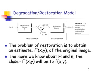
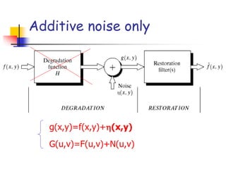
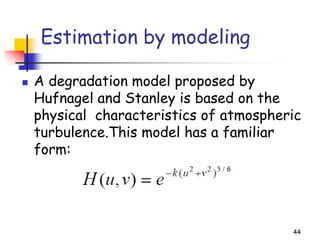
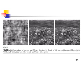
Image restoration is a process of reconstructing an image that has been degraded to recover the original image using knowledge of the degradation process. The goal is to estimate the original image by modeling the degradation and applying the inverse process. Common degradations include noise, which can be modeled statistically. Restoration techniques include spatial filters like mean, median filters to reduce additive noise, and frequency domain filters to reduce periodic noise. The degradation function must be estimated from the image, experimentally, or by modeling before applying inverse or Wiener filtering for restoration.

1. Image Restoration

2. Image Restoration
◼ Restoration is a process of reconstruction or
recovering an image that has been degraded by
using some a priori knowledge of the
degradation phenomenon.
◼ It is objective which means that restoration
techniques are oriented toward modeling the
degradation and applying the inverse process in
order to recover the original image.
2

3. Degradations

4. 4
Degradation/Restoration Model
◼ The problem of restoration is to obtain
an estimate, f^(x,y), of the original image.
◼ The more we know about H and η, the
closer f^(x,y) will be to f(x,y).

5. Degradation/Restoration Model
◼ In the Spatial domain
◼ In the Frequency domain
◼ IF we know the values of H and N, we could
recover F as given
◼ This may not practical. Even though we may have
some statistical information about the noise. As
well H(,u,v) may be close to, or equal to zero. 5
)
,
(
)
,
(
*
)
,
(
)
,
( y
x
y
x
f
y
x
h
y
x
g 
+
=
)
,
(
)
,
(
).
,
(
)
,
( v
u
N
v
u
F
v
u
H
v
u
G +
=
)
,
(
)
,
(
)
,
(
)
,
(
v
u
H
v
u
N
v
u
G
v
u
F
−
=

6. Noise Properties and models
◼ The principle source of noise arises during image
acquisition and/or transmission.
◼ Assuming noise is independent of spatial coordinates
and uncorrelated with respect to the image itself.
◼ Concerning with the statistical behavior of the gray-
level values in the noise component.
◼ Considering random variables characterized by a
Probability Density Function (PDF).
6

7. Gaussian noise
◼ It is used frequently in practice
7

8. Uniform noise







−
=
otherwise
0
if
1
)
(
b
z
a
a
b
z
p
12
)
(
2
2
2 a
b
b
a
−
=
+
=


Mean:
Variance:
◼ Less practical, used for random number
generator

9. 9
Impulse (salt-and-pepper) noise
• If b>a, gray-level b will appear
as a light dot. Conversely, level
a will appear like a dark dot if
either Pa or Pb is zero.

11. Periodic noise
◼ Arise from electrical or
electromechanical interference during
image acquisition
◼ Spatial dependence
◼ Observed in the frequency domain

12. Sinusoidal noise:
Complex conjugate
pair in frequency
domain

13. Estimation of noise parameters
◼ Periodic noise
◼ Observe the frequency spectrum
◼ Random noise with unknown PDFs
◼ Case 1: imaging system is available
◼ Capture images of “flat” environment
◼ Case 2: noisy images available
◼ Take a strip from constant area
◼ Draw the histogram and observe it
◼ Measure the mean and variance

14. Observe the histogram
Gaussian uniform

15. ◼ Histogram is an estimate of PDF
Measure the mean and variance


=
S
z
i
i
i
z
p
z )
(



−
=
S
z
i
i
i
z
p
z )
(
)
( 2
2



Gaussian: , 
Uniform: a, b

16. Restoration in the presence of noise-
spatial filtering
◼ A method of choice in situations when
only additive noise is present
◼ Enhancement and restoration become
almost indistinguishable disciplines when
only additive noise is present
16

17. Additive noise only
g(x,y)=f(x,y)+(x,y)
G(u,v)=F(u,v)+N(u,v)

18. Spatial filters for de-noising
additive noise
◼ Skills similar to image enhancement
◼ Mean filters
◼ Order-statistics filters
◼ Adaptive filters

19. Mean filters
◼ Arithmetic mean: Noise is reduced as a
result of blurring
◼ Geometric mean: It tends to lose less
image detail compared with mean filter


=
xy
S
t
s
t
s
g
mn
y
x
f
)
,
(
)
,
(
1
)
,
(
ˆ
Window centered at (x,y)
mn
S
t
s
t
s
g
y
x
f
xy
/
1
)
,
(
)
,
(
)
,
(
ˆ







=


20. Mean filters (cont.)
◼ Harmonic mean filter
◼ Contra-harmonic mean filter




+
=
xy
xy
S
t
s
Q
S
t
s
Q
t
s
g
t
s
g
y
x
f
)
,
(
)
,
(
1
)
,
(
)
,
(
)
,
(
ˆ


=
xy
S
t
s t
s
g
mn
y
x
f
)
,
( )
,
(
1
)
,
(
ˆ
Q=-1, harmonic
Q=0, airth. mean
Q=+, ?

21. 21

22. 22
Order-statistics filters
I. Median filter: provides excellent noise
reduction capabilities with considerably less
blurring than linear smoothing filters
II. Max and Min filter: Max filter is useful for
finding the brightest points. It is effective for
pepper noise
22

23. 23
Order-statistics filters
II. Max and Min filter: Min filter is useful for finding
the darkest points. It reduces salt noise
III. Midpoint filter: this filter combines order
statistics and averaging. It works well for
Gaussian and uniform noise
23

24. 24

25. 25

26. Adaptive filters
◼ The behavior changes based on statistical
characteristics of the image inside the filter
region defined by window Sxy.
◼ Its performance superior to the previous
filter
◼ Local noise reduction filter:
ML-local mean of the pixels in Sxy
26

27. Adaptive filters
- Variance of the noise to form g(x,y)
- Local variance of the pixels in Sxy
◼ If =0 → zero-noise case
◼ If >> → f^(x,y)≈g(x,y) the variance is
associated with edges; no noise
◼ If = → noise is reduced by averaging
27
2
n

2
L

2
n

2
n

2
L

2
n

2
L


28. 28

29. Periodic noise reduction
◼ Pure sine wave
◼ Appear as a pair of impulse (conjugate) in
the frequency domain
)
sin(
)
,
( 0
0 y
v
x
u
A
y
x
f +
=






+
+
−
−
−
−
= )
2
,
2
(
)
2
,
2
(
2
)
,
( 0
0
0
0






v
v
u
u
v
v
u
u
A
j
v
u
F

30. Periodic noise reduction
(cont.)
◼ Bandreject filters
◼ Bandpass filters
◼ Notch filters

31. Bandreject filters
* Reject an isotropic frequency
ideal Butterworth Gaussian

32. Bandreject filters
32

33. Bandreject filters (Cont.)

34. noisy spectrum
bandreject
filtered

35. Bandpass filters
◼ Hbp(u,v)=1- Hbr(u,v)
 
)
,
(
)
,
(
1
v
u
H
v
u
G bp
−


36. Notch filters
◼ Reject(or pass) frequencies in predefined
neighborhoods about a center frequency
ideal
Butterworth Gaussian

37. Notch filters (Cont.)

38. Notch filters (Cont.)

39. Horizontal
Scan lines
Notch
pass
DFT
Notch
pass
Notch
reject

40. Estimating the degradation function
◼ Estimation by Image observation
◼ Estimation by experimentation
◼ Estimation by modeling

41. Estimation by image observation
◼ Take a window in the image
◼ Simple structure
◼ Strong signal content
◼ Estimate the original image in the window
)
,
(
ˆ
)
,
(
)
,
(
v
u
F
v
u
G
v
u
H
s
s
s =
known
estimate

42. Estimation by experimentation
◼ If the image acquisition system is ready
◼ Obtain the impulse response
impulse Impulse response

43. Estimation by experimentation
(Cont.)
43

44. Estimation by modeling
◼ A degradation model proposed by
Hufnagel and Stanley is based on the
physical characteristics of atmospheric
turbulence.This model has a familiar
form:
44

45. Estimation by modeling
◼ Ex. Atmospheric model
6
/
5
2
2
)
(
)
,
( v
u
k
e
v
u
H +
−
=
original k=0.0025
k=0.001 k=0.00025

46. Estimation by modeling

47. Estimation by modeling

48. Estimation by modeling: example
original Apply motion model

49. Inverse filtering
◼ The simplest approach is direct inverse filtering
In the presence of noise, substituting the
following eqn. into the above Eqn.
Yields,
49

50. Inverse filtering
◼ With the estimated degradation function
H(u,v)
G(u,v)=F(u,v)H(u,v)+N(u,v)
=>
)
,
(
)
,
(
)
,
(
)
,
(
)
,
(
)
,
(
ˆ
v
u
H
v
u
N
v
u
F
v
u
H
v
u
G
v
u
F +
=
=
Estimate of
original image
Problem: 0 or small values
Unknown
noise
Sol: limit the frequency
around the origin

51. Min. Mean Square Error (Wiener)
filtering
◼ Incorporating both the degradation fn. and
statistical characteristics of noise into the
restoration process
◼ Assume noise and image are uncorrelated
◼ Based on these conditions, the minimum of the
error function is given in the frequency domain
by the expression
51

52. Min. Mean Square Error (Wiener)
filtering

53. Min. Mean Square Error (Wiener)
filtering
Where,
53
• If Sη and Sf are not known, we set ratio (Sη /Sf ) with
specified constant K
• If Sη =0 (absence of noise), the filter reduces to the ideal
inverse filter

54. 54

55. Image Restoration in Matlab

56. Image Restoration in Matlab (Cont.)