This document provides an overview of digital image processing techniques for image restoration. It defines image restoration as improving a degraded image using prior knowledge of the degradation process. The goal is to recover the original image by applying an inverse process to the degradation function. Common degradation sources are discussed, along with noise models like Gaussian, salt and pepper, and periodic noise. Spatial and frequency domain filtering techniques are presented for restoration, such as mean, median and inverse filters. The maximum mean square error or Wiener filter is also introduced as a way to minimize restoration error.

1. Digital Image Processing
Unit-3
Image Restoration
Kamlesh Kumar Pathak
Assistant Professor, Dept. of Computer Sc.& Engineering
Radha Govind Engineering College Meerut
Email: kamleshcs_1987@yahoo.co.in

2. What is Image Restoration:
Image restoration aim to improve an image in some
predefined sense.
What about image enhancement?
Image enhancement also improves an image by
applying filters.

3. Difference:
Image Enhancement --- Subjective process
Image Restoration --- Objective Process
 Restoration tries to recover / restore degraded image by using a
prior knowledge of the degradation phenomenon.
 Restoration techniques focuses on:
1. Modeling the degradation
2. Applying inverse process in order to recover the original image.

4. Model of the Image Degradation / Restoration Process

5.  Degradation function along with some additive noise operates on
f(x, y) to produce degraded image g(x, y)
 Given g(x, y), some knowledge about the degradation function
H and additive noise η(x, y), objective of restoration is to obtain
estimate f’(x, y) of the original image.
 If H is linear, position invariant process then degraded image in
spatial domain is given by:
 h(x, y) = Spatial representation of H
 * indicates convolution

6.  Since convolution in Spatial domain = multiplication in
Frequency Domain
 We Assume that H is identity operator
 We deal only with degradation due to Noise

7. Noise Models: Noise in digital image arises during
1. Image Acquisition
2. Transmission
During Image Acquisition
 Environmental conditions (Light Levels)
 Quality of sensing element
During Transmission
 Interference during transmission

8. Spatial Properties of Noise:
1. With few exception we consider that noise is independent of spatial
coordinates.
2. We assume that noise is uncorrelated with respect to the image itself
(There is no correlation between image pixels and the values of noise
components)
Fourier Properties of Noise:
 Refers to the frequency contents of noise in the Fourier sense.
 If Fourier spectrum of noise is Constant, the noise is usually called
WHITE NOISE

9. Some Noise Probability Density Functions (PDFs):
 Gaussian Noise
 Rayleigh Noise
 Erlang (Gamma) Noise
 Exponential Noise
 Uniform Noise
 Impulse (Sal & Pepper Noise)
 Periodic Noise

10. Spatial Noise Descriptor
 Statistical behavior of the gray level values in the noise
component.
 Can be considered as random variables
 Characterized by Probability Density Functions (PDFs)

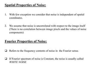
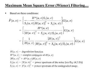
12. Gaussian / Normal Noise Model
1. Most frequently used.
2. PDF of Gaussian random variable z is given by:
 z  Gray level
 µ  Mean of average value of z
 σ  Standard Deviation of z
 σ2  Variance of z
When z is defined by this equation then
 About 70% of its values will be in the
range [(µ - σ),(µ + σ)] and
 About 95% of its values will be in the
range [(µ - 2σ),(µ + 2σ)]
Plot of function

13. Rayleigh Noise Model
PDF of Rayleigh Noise is given by:
 z  Gray level
 µ  Mean of average value of z
 σ2  Variance of z
 Basic shape of this density is skewed to
the right.
 Quite useful for approximating skewed
histograms.
Plot of function

14. Erlang (Gamma) Noise Model
PDF of Erlang Noise is given by:
 z  Gray level
 µ  Mean of average value of z
 σ2  Variance of z
 Above equation is also called
Erlang Density
 If denominator is Gamma function
then it is called Gamma density
Plot of function
 a > 0
 b = positive integer

15. Exponential Noise Model
PDF of Exponential Noise is given by:
 z  Gray level
 µ  Mean of average value of z
 σ2  Variance of z
 a > 0
 Special case of Erlang Density
Where b=1
Plot of function

16. Uniform Noise Model
PDF of Uniform Noise is given by:
 z  Gray level
 µ  Mean of average value of z
 σ2  Variance of z
Plot of function

17. Impulse (Salt & Pepper) Noise Model
PDF of Uniform Noise is given by:
 z  Gray level
 If b > a then b  light dot and a dark
dot
 If either Pa or Pb = 0  Unipolar
Impulse Noise otherwise Bipolar
Impulse Noise.
 If Neither probability is 0 and approximately equal then noise values will
resemble salt & pepper granules randomly distributed over the image.
 Also referred as Shot and Spike Noise
Plot of function

18. This test pattern is well-suited for illustrating the noise models, because it is composed
of simple, constant areas that span the grey scale from black to white in only three
increments. This facilitates visual analysis of the characteristics of the various noise
components added to the image.
Example

21. Restoration using Spatial Filtering
We can use spatial filters of different kinds to remove different
kinds of noise.
Arithmetic Mean Filter
Let Sxy represents the set of coordinates in a rectangular sub
image window of size m x n centred at (x, y).
This filter computes the average value of the corrupted image in
the area defined by Sxy.


xySts
tsg
mn
yxf
),(
),(
1
),(ˆ 1/9
1/9
1/9
1/9
1/9
1/9
1/9
1/9
1/9
Implemented as simple smoothing filter
Well Suited for Gaussian / Uniform Noise

22. Geometric Mean Filter
Each restored pixel is given by the product of the pixels in the
sub image window, raised to the power 1/mn.
Achieves smoothing comparable to Arithmetic Mean Filter but
tends to lose less image details in the process.
Well Suited for Gaussian / Uniform Noise
mn
Sts xy
tsgyxf
1
),(
),(),(ˆ








 

23. Harmonic Mean Filter
Works well for salt noise but fails for pepper noise.
Also does well for Gaussian Noise


xySts tsg
mn
yxf
),( ),(
1
),(ˆ

24. Example:
Original
Image
Image
Corrupted
By Gaussian
Noise
After A 3*3
Geometric
Mean Filter
After A 3*3
Arithmetic
Mean Filter

25. Order Statistic Filter
Result is based on the ranking / ordering of the pixels contained
in the image area encompassed by the filter.
Median Filter
)},({),(ˆ
),(
tsgmedianyxf
xySts 

Effective for both uni-polar and bipolar impulse noise.
Excellent at noise removal, without the smoothing effects that
can occur with other smoothing filters

26. Max Filter Good for Pepper Noise
Min Filter Good for Salt Noise
)},({max),(ˆ
),(
tsgyxf
xySts 

)},({min),(ˆ
),(
tsgyxf
xySts 


27. Mid Point Filter Good for Gaussian / Uniform Noise



 

)},({min)},({max
2
1
),(ˆ
),(),(
tsgtsgyxf
xyxy StsSts

28. Image
Corrupted
By Salt And
Pepper Noise
Result of 1
Pass With A
3*3 Median
Filter
Result of 2
Passes With
A 3*3 Median
Filter
Result of 3
Passes With
A 3*3 Median
Filter
Example:

29. Image
Corrupted
By Pepper
Noise
Image
Corrupted
By Salt
Noise
Result Of
Filtering
Above
With A 3*3
Min Filter
Result Of
Filtering
Above
With A 3*3
Max Filter
Example:

30. Image
Corrupted
By Uniform
Noise
Image Further
Corrupted
By Salt and
Pepper Noise
Filtered By
5*5 Arithmetic
Mean Filter
Filtered By
5*5 Median
Filter
Filtered By
5*5 Geometric
Mean Filter
Filtered By
5*5 Alpha-Trimmed
Mean Filter
Example (Combined):

31. Periodic Noise
Typically arises due to electrical / Electro-
mechanical interference during image
acquisition.
Spatially dependent noise.
Can be reduced significantly via Frequency
Domain Filtering.
Parameters can be estimated by inspecting
the Frequency Spectrum of the image.
Periodic noise tend to produce frequency
spikes
Image corrupted by
Sinusoidal noise
Spectrum (Each pair of
conjugate impulses
corresponds to one sine wave)

32. Periodic Noise Reduction by Frequency Domain Filtering
Removing periodic noise form an image involves removing a
particular range of frequencies from that image
Bandreject Filter
Bandpass Filters
Notch Filter

33. Bandreject Filter
Removes / Attenuates a band of frequencies about the origin of the Fourier
Transform.
Ideal Bandreject Filter:












2
),(1
2
),(
2
0
2
),(1
),(
0
00
0
W
DvuDif
W
DvuD
W
Dif
W
DvuDif
vuH
D(u, v) = Distance of point from the origin
W = Width of the band
D0 = Radial Centre

34. Butterworth Bandreject Filter:
Gaussian Bandreject Filter:

35. Ideal Band
Reject Filter
Butterworth
Band Reject
Filter (of order 1)
Gaussian
Band Reject
Filter

36. Image corrupted by
sinusoidal noise
Fourier spectrum of
corrupted image
Butterworth band
reject filter
Filtered image
Example:

37. Inverse Filtering
An approach to restore an image.
Compute an estimate F’( u, v) of the transform of the original image by:
Divisions are made between individual elements of the functions.

38. Inverse Filtering…
Above Equation concludes that:
Even if we know degradation function, we can not recover the undegraded
image [Inverse Fourier Transform of F(u, v)] exactly because
N(u, v) is random function whose Fourier Transform is not known.
If degradation has ZERO or less value then N(u, v) / H(u, v) dominates the
estimated F’(u, v).
No explicit provision for handling Noise.

39. Maximum Mean Square Error (Wiener) Filtering
 Incorporates both degradation function and statistical characteristics of
noise into restoration process.
 Considers images and noise as random process.
 Find an estimate f’ of the uncorrupted image f such that mean square error
between them is minimized. Error measure is given by:
 E{.} = Expected value of the argument
 Assumptions:
 image and noise are uncorrelated.
 One or other has Zero mean
 Gray levels in the estimate are a linear function of levels in the
degraded image.

40. Maximum Mean Square Error (Wiener) Filtering…
 Based on these conditions:

41. Singularity & Ill-condition?
Today After Lunch