This experiment aims to study the frequency response of lag and lead compensators. A lag compensator circuit contains resistors and capacitors, while a lead compensator contains resistors and an inductor. These compensator circuits are connected to a function generator and digital storage oscilloscope. The transfer functions of the lag and lead compensators are derived. For the lead compensator, the pole-zero plot is drawn to show that the zero is closer to the origin than the pole, introducing positive phase angle. By measuring the output waveforms on the oscilloscope for different compensator circuits, the effect of lag and lead compensation on the frequency response is observed experimentally.

1. Experiment No. 1
AIM :-
Experimental determination of Dc servo motor parameters for mathematical modeling,
transfer function and characteristics
APPARATUS:-DC servo motor kit
THEORY:- DC servo motors are normally used as prime movers in computers, numerically
controlled machinery, or other applications where starts and stops are made quickly and accurately.
Servo motors have lightweight, low-inertia armatures that respond quickly to excitation-voltage
changes. In addition, very low armature inductance in these servo motors results in a low electrical
time constant (typically 0.05 to 1.5 msec) that further sharpens servo motor response to command
signals. Servo motors include permanent-magnet, printed-circuit, and moving-coil (or shell) dc
servo motors. The rotor of a shell dc servo motor consists of a cylindrical shell of copper or
aluminum wire coils which rotate in a magnetic field in the annular space between magnetic pole
pieces and a stationary iron core. The servo motor features a field, which is provided by cast
AlNiCo magnets whose magnetic axis is radial. Servo motors usually have two, four, or six poles.
Dc servo motor characteristics include inertia, physical shape, costs, shaft resonance, shaft
configuration, speed, and weight. Although these dc servo motors have similar torque ratings, their
physical and electrical constants vary.
As compared to ordinary DC motors, the DC servomotors have to be specially designed
particularly with physical dimensions. The DC servomotors are generally large in length and
smaller in diameter.
A conventional motor is essentially a constant speed motor running at or near its rated speed
and hence designed specifically to yield optimum performance near about rated speed. Steady state
characteristics of the motor are important, transient response being relatively unimportant. Since
a servomechanism is an error actuated control system which operates to reduce its actuating speed
or signal to zero. The servomotor runs with zero speed as its basic speed. It may make few
revolutions in the forward direction at the speed determined by the magnitude of the actuating
signal and then suddenly rotates in opposite directions the sign of the actuating signal changes. It
is in a transient state of operation. Hence the transient of the motor is of vital importance.
In order to cope up with such a duty, servomotor must satisfy the requirement listed below:-
A) It should be easily reversible and capable of being easily controlled over a wide range of
speeds in either direction.
B) It should respond quickly in order to follow varying control signals. To fulfill this
characteristics following are the requirements:-

2. 1. It should have a high torque to inertia ratio so that it may accelerate fast. The moment of
inertia of the rotor varies as D2, while the torque developed varies as L, where D is the
diameter of the rotor and L is axial length. D is reduced in order to reduce inertia, while
the axial length is increased to increase the developed torque.
2. It should have a stable speed characteristic i.e. the increase in output torque should be
followed by decrease in speed of motor. In other way it can be seen that a speed torque
characteristic with a negative slope introduces positive damping in the system and thus
helps to stabilize
Armature controlled dc servomotor
Modeling and Transfer function:
The following are the assumptions in deriving the transfer function of armature controlled dc
servomotor.
1. Airgp flux is proportional to field current
2. Armature reaction is negligibly small
3. Back emf is proportional to speed
4 The field current is constant.
Let Ra = Armature resistance,
La = Armature inductance
J= total M.I of the rotor.
θ = shaft position
Va = Voltage applied to armature
Ia = Armature current
f = Coefficient of viscous friction
Ra
Va
La
θ
ia
If constant
Vf

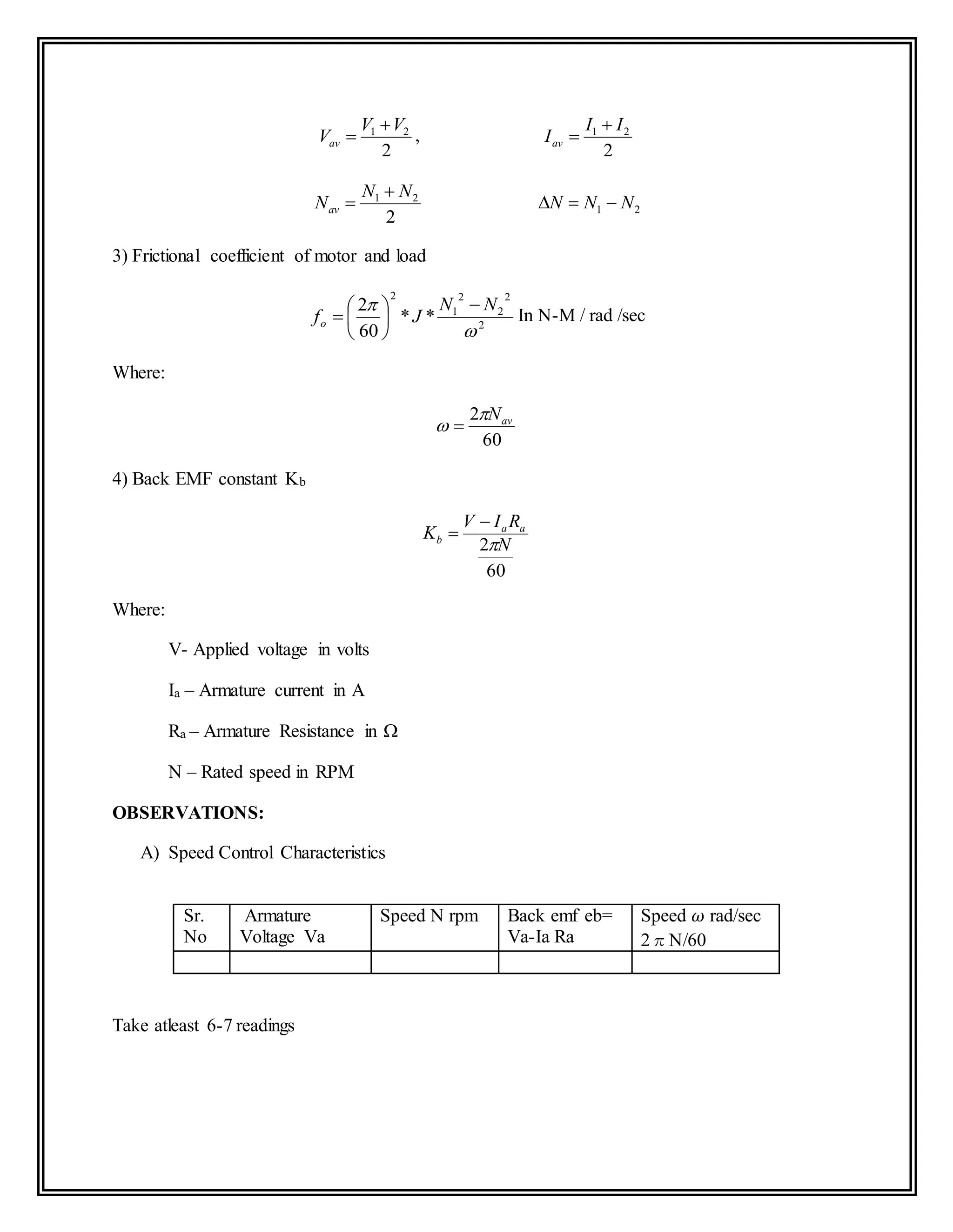
3. The Voltage equation of the motor is given by
Va = Eb + Ia Ra + La dIa / dt, taking Laplace transform on both sides,
Va(s) = Eb(s)+ Ia ( Ra+ s La)
Ia(s) = (Va - Eb(s) / ( Ra+ s La)……………………………….(1)
Electromagnetic torque developed is given by;
Te α φ. Ia
Te = Kt. Ia……………………… since φ is constant
Or Tm(s) = Kt. Ia(s)……………………………………….(2)
But the motor torque developed has to satisfy following equation
Tm = J.d2θ /dt2 + f. d θ /dt + TL
Or Te(s) = [ J s2 + f(s) ] θ(s)………………………………..(3)
Equating (2) and (3), we get,
Kt. Ia(s) = [ J s2 + fs ] θ(s)
Kt [ (Va - Eb(s) / (Va - Eb(s) ] = = [ J s2 + fs ] θ(s)…….(4)
But the back emf is proportional to motor speed ,
Eb α Kb . d θ /dt .
Eb = Kb. d θ /dt
where, Kb is back emf constant and expressed as volts / rad. / sec
Or Eb(s) = s.Kb. θ(s)…………………………………………(5)
Sub. (5) in (4 ) and simplification yields,
G(s) =)θ(s) / Va(s) = Kt / ( J s2 + fs ) ( Ra+ s La) s. Kt. Kb ……(6)
Equ. (6) is the required transfer function of

4. Armature controlled dc servo motor and can be represented by block diagram as shown in fig
blow
Consider T. F of the system
G(s) =θ(s) / Va(s) = Km / ( J s2 + fs ) ( Ra+ s La) s. Km. Kb
Quantities involved in the above equation are j, Ra, La, Km, and Kb. Out of this Ra and La can
be determined by conventional method
J ( mechanical inertia ) can be determined by retardation test, Now
Eb = Kb.ω = Kb 2ПN /60 -----------------(a)
Electrical equivalent of mechanical power developed by motor = Eb. Ia
Eb. Ia = (2ПN. Tm /60 ) , substituting Eb from (a)
( Kb 2ПN /60 ) Ia = (2ПN. Tm /60 ) Tm
But Te = Kt.Ia…………………from (2)
( Kb 2ПN /60 ) Ia = (2ПN. Tm /60 ) Km Ia
So the only unknown quantities are Kb and f
Determination of Kb and Kt
Back emf constant (Kb)
First the motor is run on no load at constant excitation. Various speeds at different applied
voltages are noted down. Then graph is plotted showing back emf ( Eb = Va- Ia.Ra) against speed.
The slope of the curve gives Kb.
1 / ( Ra+ s La) 1 / (J s + f)Kt 1 / s
Kb(s)
Tm(s)Ia(S) Sθ(s)
+
-
Kb = Kt

5. Motor torque constant (Tm)
Te= Kt.Ia
and Tm is also equal to Eb.Ia/ ω
slope of the graph between Tm and Ia gives Motor torque constant (Tm)
Inertia constant: J
The inertia can be determined by a retardation test. The test works on the principle
that when a motor is switched off from the mains it decelerates and comes to rest.
The angular retardation at any speed is proportional to the retarding torque and is
inversely proportional to the inertia. The torque lost at any speed is calculated by
running the motor at that speed steadily on no load and noting the power input.
From this power the losses that takes place in the armature and field are deducted
to get the power converted into mechanical form. All this power is spent in over
coming the mechanical losses at that speed. This can be repeated at any defined
speed to get the lost power (PL) and torque lost (Tlost) due to mechanical losses.
In a retardation test the motor speed is taken to some high value and the power to
the motor is switched off. The torque required by the losses is supplied by the
energy stored in the motor inertia. The lost torque at any speed can be written as
PL = Tlost.ω
Tlost = PL/w = J dw/dt
Here the dw/dt is the slope of the retardation curve and the (Tlost) is the torque required to be
met at the given speed. From these values the moment of inertia can be computed as
J = Tlost/(dw/dt) = PL/( w. dw/ dt) kgm2
21
21
2
2
60
*
*
tt
tt
NN
IV
J
av
avav










In Kg/m2
Where:
T1 – Time for fall of speed from N1 to N2 in no load condition
T2 – Time for fall of speed from N1 to N2 in load condition

6. 2
21 VV
Vav

 ,
2
21 II
Iav


2
21 NN
Nav

 21 NNN 
3) Frictional coefficient of motor and load
2
2
2
2
1
2
**
60
2

 NN
Jfo







 In N-M / rad /sec
Where:
60
2 avN
 
4) Back EMF constant Kb
60
2 N
RIV
K aa
b



Where:
V- Applied voltage in volts
Ia – Armature current in A
Ra – Armature Resistance in 
N – Rated speed in RPM
OBSERVATIONS:
A) Speed Control Characteristics
Sr.
No
Armature
Voltage Va
Speed N rpm Back emf eb=
Va-Ia Ra
Speed 𝜔 rad/sec
2πN/60
Take atleast 6-7 readings

7. b) Load Characteristics
Sr.
No
Motor voltage (volts) Current Ia
(amp)
Speed
rad/sec
Load Tm =
9.81*(S1-
S2)*r
N-M
S1 Kg S2
Kg
r= radius of break drum in m
Take atleast 6-7 readings
Result table
Sr.
No
Va
volts
Ia
Amps
W
Rad/sec
Eb
volts
Tm
N-m
Km
N-M/Amp
Kb
V/rad/sec
Determination of Constants
Constant From Graph Avg Value
(observed)
Kt
Kb
J --
B --
Ra --
La --
Determined Transfer function G(s) =………………………
Conclusion:
Experiment No. 2

8. AIM:-
Experimentalstudyof time responsecharacteristicsof R-L-Csecondordersystem.Validationusing
simulation.
APPARATUS:-R,L,C components, Function generator, DSO
Circuit/ Set-up:
Theory:
Circuitscontainingtwoinductorsortwocapacitorsorone of eachalsoexhibitatransientresponsebefore
theyreach steady-state.However,asthese circuitsare more complex,theirresponsemighttake various
forms that mainly depend on the respective values of R, L and C. Figure 2.2 shows the characteristic
responses for a second-order circuit to a step input function applied at t=0.
LR
i (t)
+ Function
Generator
V
vR(t) vL(t)
Digital
Storage
Oscilloscope
C
vC(t)
Response
Fig 2.1: Expt. setup
Fig 2.2: Effect of damping ratio on time response

9. 1. In the figure 2.3 RLC series circuit is ergized by a step voltage of V volts at t = 0, Determine the
solutions i(t) for under damped second order system. by classical or By LT method
2. Calculate damping ration for over damped, critically damped and under damped cases using selected
values of R, L and C used during experimentat
In figure 2.3, by applying KVL,
v(t)=R i(t)+L
di
dt
+
1
C
∫ i(t)dt
Taking Laplace transform
Ls I(s)+R I(s)+
1
Cs
I(s) =V(s)
Output voltage across capacitor
𝑽 𝒐( 𝒔) =
1
Cs
I(s)
Transfer function is written as
Vo(s)
V(s)
=
1
LC⁄
s2+
R
L
s+1
LC⁄
Damping Ratio 𝜻 =
𝑹
𝟐
√
𝑪
𝑳
Natural Frequency ωn=
1
√LC
Procedure :
I) Select the values of R,L,C components from the RLC load Box for each case namely under
damped, over damped and critically damped system.
II) Prepare expt set up as shown in figure.
III) Select the voltage magnitude of function generator square wave and set the frequency around 50
Hz.
IV) Connect Input from function generator to Channel I of DSO and connect channel II of DSO
across capacitance
V) Observe the Vc(t) on CRO and measure the time response parameters. If needed, adjust the
frequencyadjustment knob to adjust the ONtime of the square wave in such a waythat the transient
response settles completely
vC(t)
vR(t) vL(t)
LRt=0
i (t)+ V
-
C
Fig 2.3 RLC response calculation

10. VI) Trace the response from the CRO. Measure the following quantities (whichever is
Possible) directly from the CRO.
a) Delay time, td b) Rise time, tr c) Peak time, tp d) Maximum overshoot, Mp e)
Setting time, ts
VII) Repeat steps V and VI for different damping ratio values.
Observations :
Part A
Waveformresponse observedonCROfordifferentvaluesof R, L and C selected
A. Underdampedcase:
1. R=……..,
2. L=………..
3. C=…………..
4. DampingRatio=…………..
B. Overdampedcase
1. R=……..,
2. L=………..
3. C=…………..
4. DampingRatio=…………..
C. Criticallydampedcase
1. R=……..,
2. L=………..
3. C=…………..
4. DampingRatio=…………..
Response asseenonDSO
Response asseenonDSO
Response asseenonDSO

11. PART B
(Carry outsimulation of R-L-Cseries circuit on MATLAB fordifferentvaluesof R.)
Attach SimulinksimulationfileandresultsforRLCseriescircuitforall fourcases of damping

12. Experiment No. 3
AIM :-
Experimental Frequency Response of Lag and Lead Compensator
APPARATUS:-Lag, Lead circuit, Function generator, DSO
Laboratory setup:
Theory:
Phase Lead Compensation
A system which has one pole and one dominating zero (the zero which is closer to the origin than
all over zeros is known as dominating zero.) is known as lead network. If we want to add a
dominating zero for compensation in control system then we have to select lead compensation
network.The basic requirement of the phase lead network is that all poles and zeros of the transfer
functionof the networkmustlie on (-)ve real axisinterlacingeachotherwitha zerolocatedat the origin
of nearest origin.
Given below is the circuit diagram for the phase lead compensation network.
LAG/LEAD
Network
Digital storage
Oscilloscope
Function
Generator
InputOutput

13. From above circuit we get,
Equating above expression of I we get,
On substituting the α = (R1 +R2)/ R2 & T = {(R1R2) /(R1 +R2)} in the above equation. Where T and
α are respectively the time constant and attenuation constant, we have
The above network can be visualized as an amplifier with a gain of 1/α. Let us draw the pole
zero
plot for the above transfer function
Pole Zero Plot of Lead Compensating Network Clearlywe have -1/T (which is a zero of the transfer
function) is closer to origin than the -1/(αT) (which is the pole of the transfer function).Thus we

14. can say in the lead compensator zero is more dominating than the pole and because of this lead
network introduces positive phase angle to the system when connected in series.
Let us substitute s = jω in the above transfer function and also we have α < 1. On finding the
phase angle function for the transfer function we have
Now in order to find put the maximum phase lead occurs at a frequency let us differentiate this
phase function and equate it to zero. On solving the above equation we get
Where, θm is the maximum phase lead angle. And the corresponding magnitude of the transfer
function at maximum θm is 1/a.
The Bode plots of lead compensator are shown below
Effect of Phase Lead Compensation
1. The velocity constant Kv increases.
2. The slope of the magnitude plot reduces at the gain crossover frequency so that relative
stability improves & error decrease due to error is directly proportional to the slope.

15. 3. Phase margin increases.
4. Response become faster.
Advantages of Phase Lead Compensation
Let us discuss some of the advantages of the phase lead compensation-
1. Due to the presence of phase lead network the speed of the system increases because it
shifts gain crossover frequency to a higher value.
2. Due to the presence of phase lead compensation maximum overshoot of the system
decreases.
Disadvantages of Phase Lead Compensation
Some of the disadvantages of the phase lead compensation -
1. Steady state error is not improved.
Phase Lag Compensation
A systemwhich has one zero and one dominating pole ( the pole which is closer to origin that all
other poles is known as dominating pole) is known as lag network. Ifwe want to add a dominating
pole for compensation in control system then, we have to select a lag compensation network.
The basic requirement of the phase lag network is that all poles & zeros of the transfer function
of the network must lie in (-)ve real axis interlacing each other with a pole located or on the
nearest to the origin. Given below is the circuit diagramfor the phase lagcompensation network.
Phase Lag Compensating Network We will have the output at the series combination of the
resistor R2 and the capacitor C. From the above circuit diagram, we get

16. Now let us determine the transfer function for the given network and the transfer function can
be determined by finding the ratio of the output voltage to the input voltage.
Taking Laplace transform of above two equation we get,
On substituting the T = R2C and β = {(R2 + R1 ) / R1} in the above equation (where T and β are
respectively the time constant and dc gain), we have
The above network provides a high frequency gain of 1 / β. Let us draw the pole zero plot for
the
above transfer function. Pole Zero Plot of Lag Network Clearly we have -1/T (which is a zero of
the transfer function) is far to origin than the -1 / (βT)(which is the pole of the transfer function).
Thus we can say in the lag compensator pole is more dominating than the zero and because of
this lag network introduces negative phase angle to the system when connected in series.

17. Let us substitute s = jω in the above transfer function and alsowe have a < 1. On finding the phase
angle function for the transfer function we have
Now in order to find put the maximum phase lag occurs at a frequency let us differentiate this
phase function and equate it to zero. On solving the above equation we get
Where, θm is the maximum phase lead angle. Remember β is generally chosen to be greater than
10.
Effect of Phase Lag Compensation
1. Gain crossover frequency increases.
2. Bandwidth decreases.
3. Phase margin will be increase.
4. Response will be slower before due to decreasing bandwidth, the rise time and the settling
time become larger.
Advantages of Phase Lag Compensation
Let us discuss some of the advantages of phase lag compensation -

18. 1. Phase lag network allows low frequencies and high frequencies are attenuated.
2. Due to the presence of phase lag compensation the steady state accuracy increases.
Disadvantages of Phase Lag Compensation
Some of the disadvantages of the phase lag compensation -
1. Due to the presence of phase lag compensation the speed of the system decreases.
Experimental Procedure:
1. Connections are to be made as per the setup given before theory.
2. Input of the circuit is connected to function generator as well to Channel of DSO(digital
storage oscilloscope)
3. Output of the circuit is connected to second channel of DSO
4. The magnitude of input signal is fixed and input signal frequency is varied
5. For each frequency of the input signal connected, output(Vo) and phase is measured
from DSO
6. Reading are tabulated the table mentioned above
7. Magnitude is calculated in db
8. Magnitdue plot ( frequency vs Magnitude) and the phase plot ( frequency vs phse) are
drawn on semi log paper
9. Calculate PM, GM, Wgc and Wpc are compared with the bode plot drawn in MATLAB
using transfer function
Results:
Take readings for minimum 25 different frequencies for both Lag as well as lead
Lag Network
Reading
no
Frequency(Hz) Input(Vi)
Volts(p-p)
Output(Vo)
volts(p-p)
Magnitude
M=20log(Vo/Vi)
dB
Phase
degree
Lead Network
Reading
no
Frequency(Hz) Input(Vi)
Volts(p-p)
Output(Vo)
volts(p-p)
Magnitude
M=20log(Vo/Vi)
dB
Phase
degree
Graph:
Draw bode plot for both compensator
Conclusion:
Lag compensator acts as low pass filter and adds phase lag in the system. Lead compensator
acts as high pass filter and adds phase lead in the system.

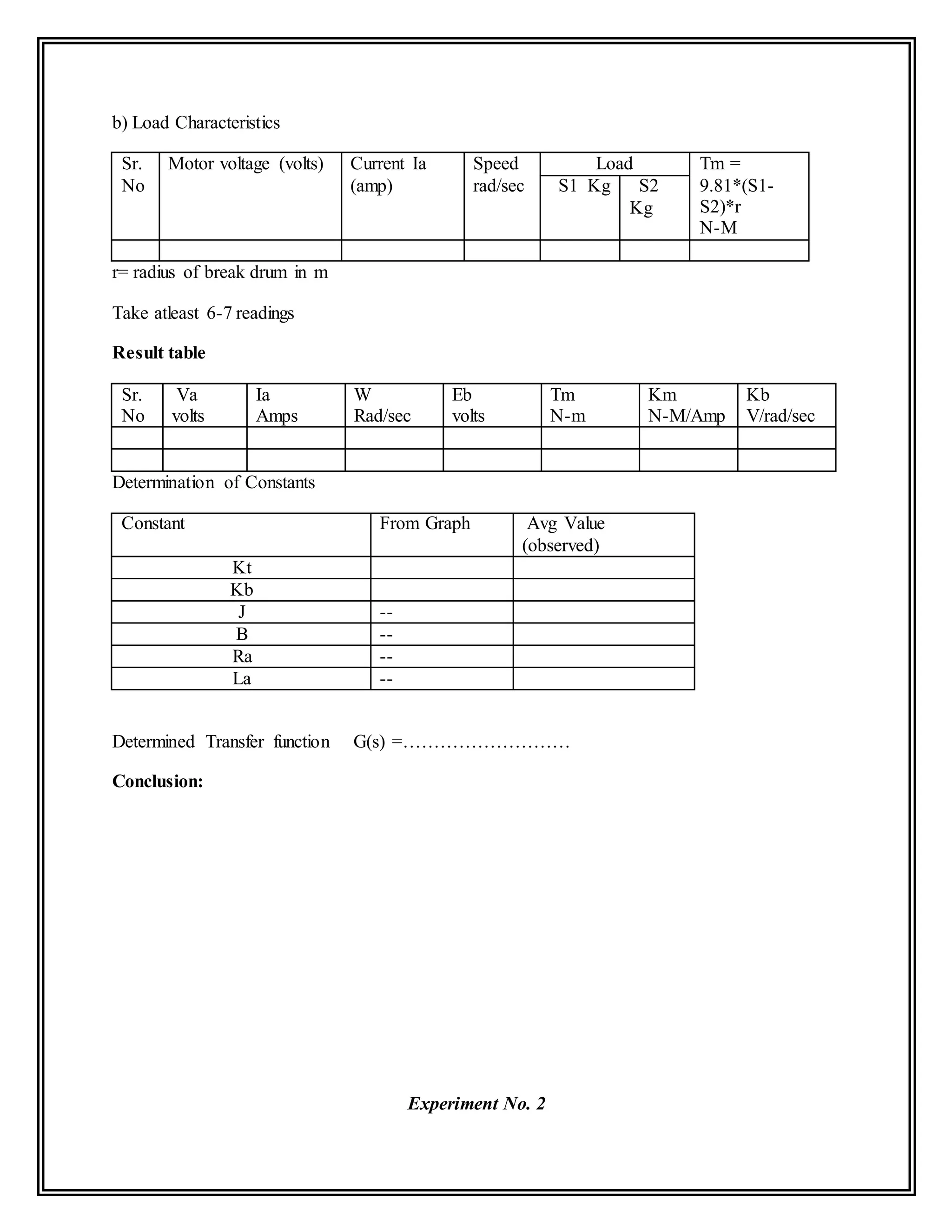
19. Experiment No. 4
AIM :- To study simulation of PID Controller using Matlab.
APPARATUS:-
THEORY:- Controller is a device which when introduced in feedback or forward path of system
controller, the steady state and transient part of device converts the input to the controller to
some otherformthan proportional toerror.Due towhichthe steadystate andtransientresponse
gets improved. In most of the practical systems, controllers input is proportional to error
generated, such systems are called as ‘Proportional error constants.’ To improve the transient
response PID controllers are introduced.
The different types of controllers are:
1) PD – Proportional + Derivative
2) PI – Proportional + Integral
3) PID – Proportional + Integral + Derivative
1) PD Controller- Thisisthe controllerinforwardpath whichchangesthe controllerinputtoPD
of error signal.
Input to controller = 𝑲 𝒑 𝒆( 𝒕) + 𝑲 𝒅
𝒅𝒆(𝒕)
𝒅𝒕
Taking Laplace, we get
Input = KpE(s) + S Kd E(s)
= E(s) [Kp + S Kd]
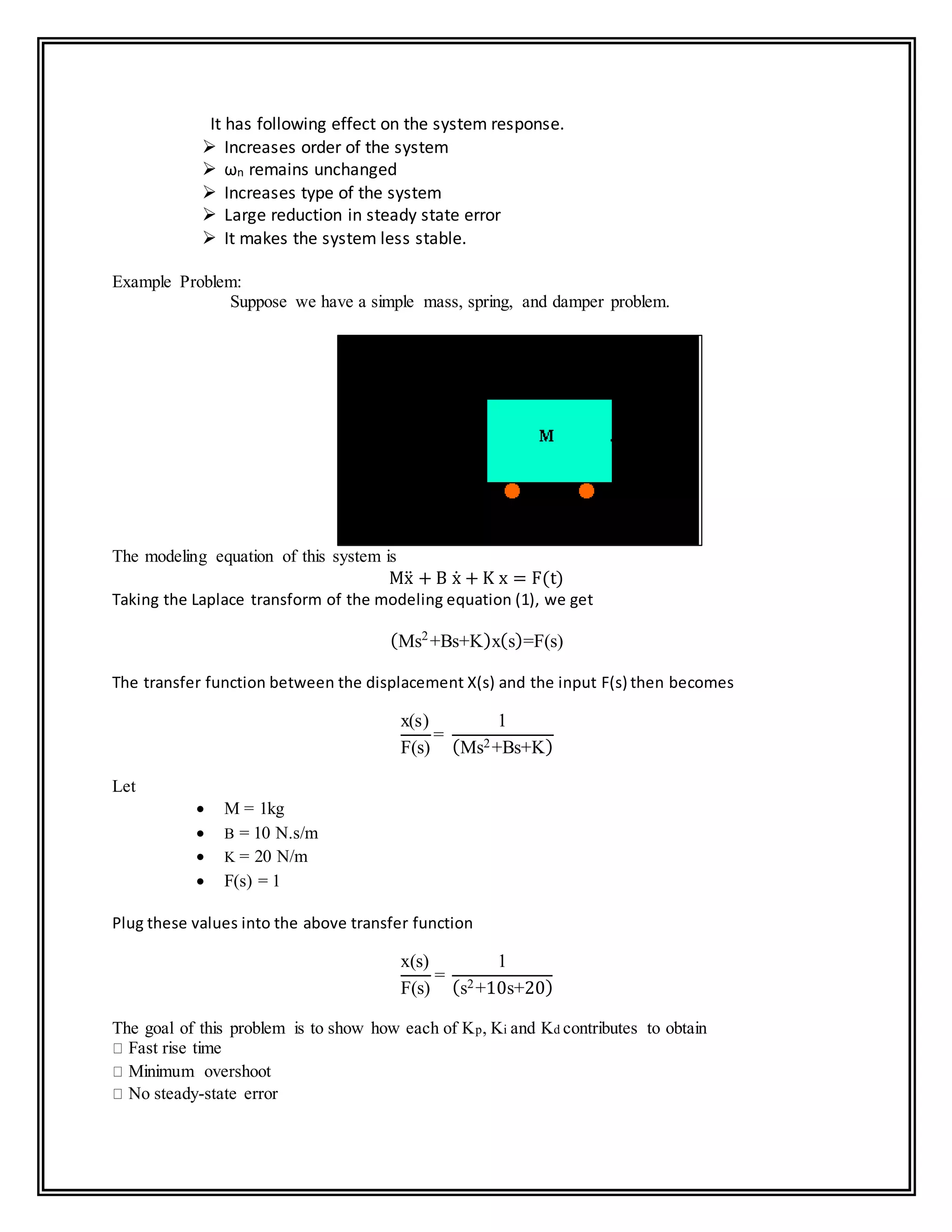
It has following effect on the system response.
 Increases damping ratio
 ωn remains unchanged
 Reduces peak overshoot
 Reduces settling time
In general it improves the transient part and not the steady state part. The type of
the system and steady state error remains unchanged.
2) PI Controller- This is the controller in forward path which changes the controller input to PI
of error signal.
Input to controller = 𝑲 𝒑 𝒆( 𝒕) + 𝑲𝒊 ∫ 𝒆( 𝒕) 𝒅𝒕
Taking Laplace, we get
Input = KpE(s) + S Ki
𝑬(𝒔)
𝒔
= E(s) [ Kp +
𝑲 𝒊
𝑺
]

20. It has following effect on the system response.
 Increases order of the system
 ωn remains unchanged
 Increases type of the system
 Large reduction in steady state error
 It makes the system less stable.
Example Problem:
Suppose we have a simple mass, spring, and damper problem.
The modeling equation of this system is
Mẍ + B ẋ + K x = F(t)
Taking the Laplace transform of the modeling equation (1), we get
(Ms2
+Bs+K)x(s)=F(s)
The transfer function between the displacement X(s) and the input F(s) then becomes
x(s)
F(s)
=
1
(Ms2+Bs+K)
Let
 M = 1kg
 B = 10 N.s/m
 K = 20 N/m
 F(s) = 1
Plug these values into the above transfer function
x(s)
F(s)
=
1
(s2+10s+20)
The goal of this problem is to show how each of Kp, Ki and Kd contributes to obtain
Fast rise time
Minimum overshoot
No steady-state error

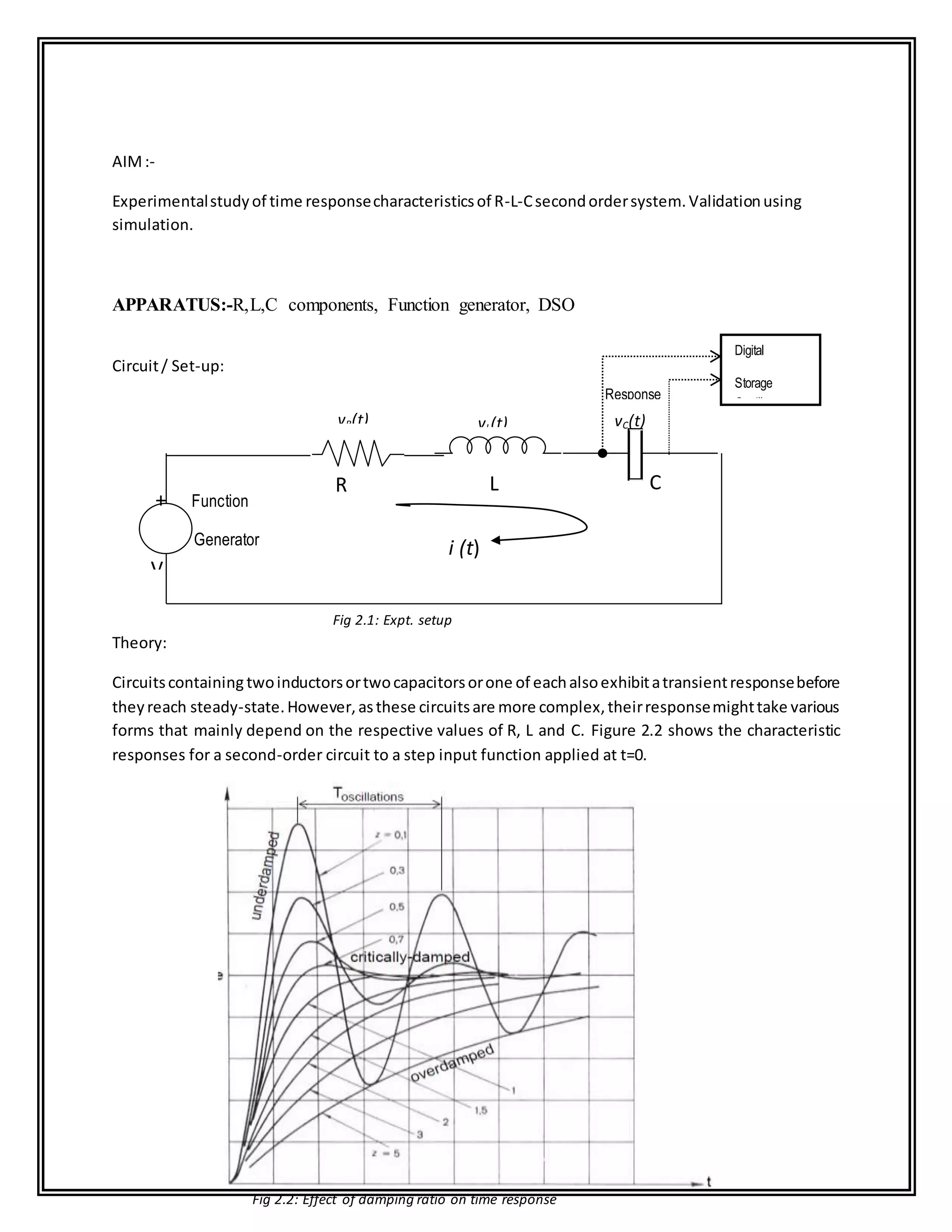
21. Open-loop step response: Let's first view the open-loopstep response.
num=1;
den=[1 10 20];
plant=tf(num,den);
step(plant)
MATLAB command window should give you the plot shown below.
The DC gain of the plant transfer function is 1/20, so 0.05 is the final value of the output to a unit
step input. This corresponds to the steady-state error of 0.95, quite large indeed.Furthermore, the
rise time is about one second, and the settling time is about 1.5 seconds. Let's design a controller
that will reduce the rise time, reduce the settling time,and eliminates the steady-state error.
Proportional control:
The closed-looptransfer function of the above system with a proportional controller is:

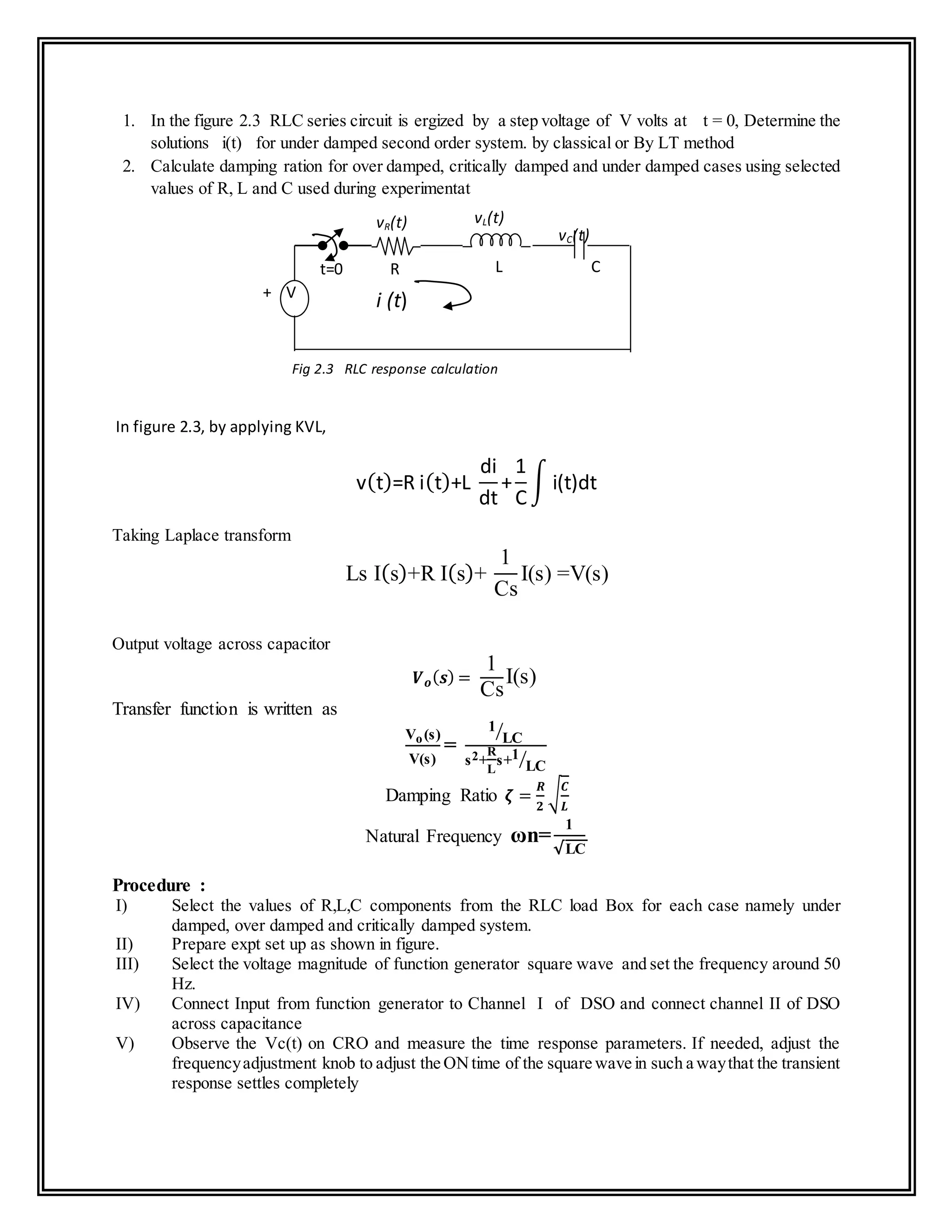
22. Let the proportional gain (KP) equal 300:
Kp=300;
contr=Kp;
sys_cl=feedback(contr*plant,1);
t=0:0.01:2;
step(sys_cl,t)
The above plot shows that the proportional controller reduced both the rise time and the steady-
state error, increased the overshoot, and decreased the settling time by small amount.
Proportional-Derivative control:
The closed-looptransfer function of the given system with a PD controller is:
Let KP equal 300 as before and let KD equal 10.
Kp=300;
Kd=10;
contr=tf([Kd Kp],1);
sys_cl=feedback(contr*plant,1);
t=0:0.01:2;

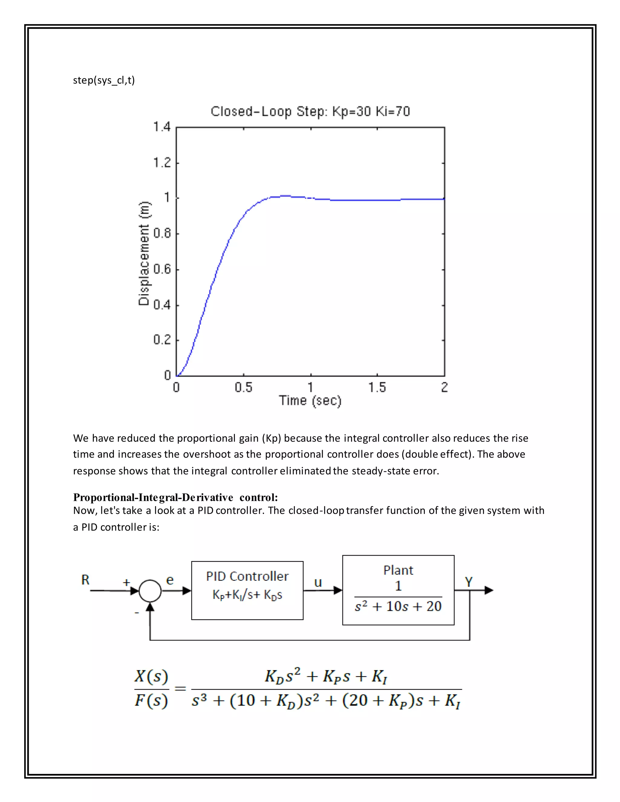
23. step(sys_cl,t)
This plot shows that the derivative controller reduced both the overshoot and the settling time, and
had a small effect on the rise time and the steady-state error.
Proportional-Integral control:
Before going into a PID control, let's take a look at a PI control. For the givensystem, the closed-
loop transfer function with a PI control is:
Let's reduce the KP to 30, and let KI equal 70.
Kp=30;
Ki=70;
contr=tf([Kp Ki],[1 0]);
sys_cl=feedback(contr*plant,1);
t=0:0.01:2;

24. step(sys_cl,t)
We have reduced the proportional gain (Kp) because the integral controller also reduces the rise
time and increases the overshoot as the proportional controller does (double effect). The above
response shows that the integral controller eliminatedthe steady-state error.
Proportional-Integral-Derivative control:
Now, let's take a look at a PID controller. The closed-looptransfer function of the given system with
a PID controller is:

25. After several trial and error runs, the gains Kp=350, Ki=300, and Kd=50 provided the desired
response. To confirm, enter the following commands to an m-file and run it in the command window.
You should get the following step response.
Kp=350;
Ki=300;
Kd=50;
contr=tf([Kd Kp Ki],[1 0]);
sys_cl=feedback(contr*plant,1);
t=0:0.01:2;
step(sys_cl,t)
Now, we have obtained a closed-loop system with no overshoot, fast rise time, and no steady-state
error.
The characteristics of P, I, and D controllers:
The proportional controller (KP) will have the effect of reducing the rise time and will reduce, but
never eliminate, the steady state error. An integral controller (KI) will have the effect of eliminating
the steady state error, but it may make the transient response worse. A derivative control (KD) will
have the effect of increasing the stability of the system, reducing the overshoot and improving the
transient response.
Effect of each controller KP,KI and KD on the closed-loop system are summarized below