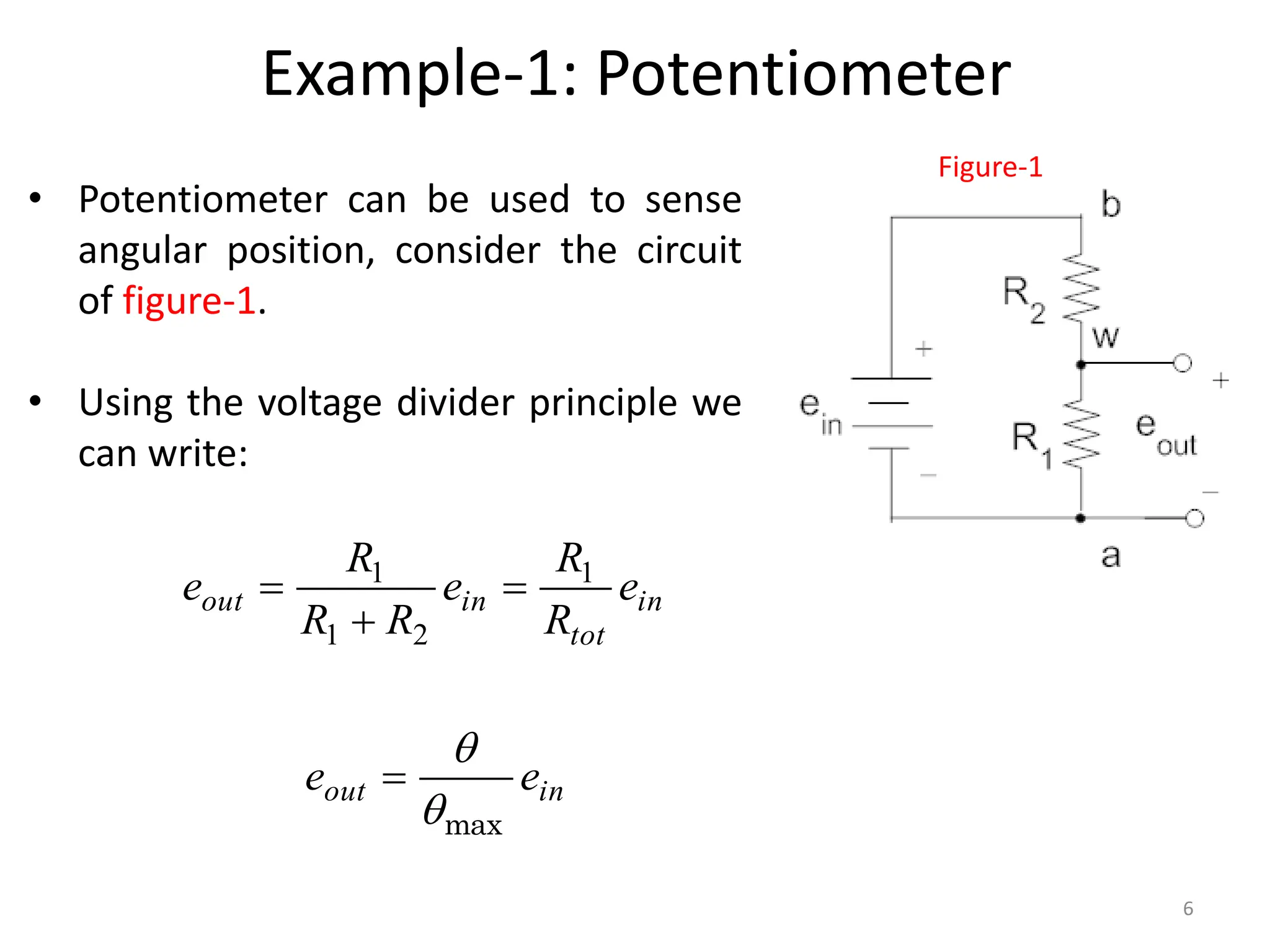
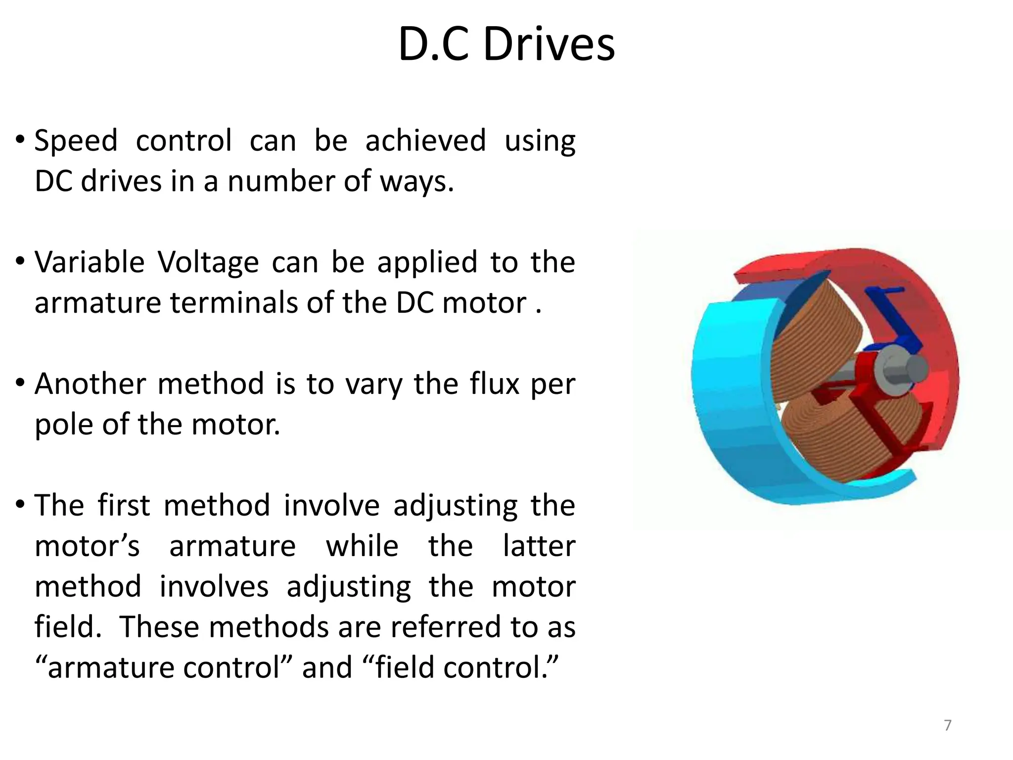
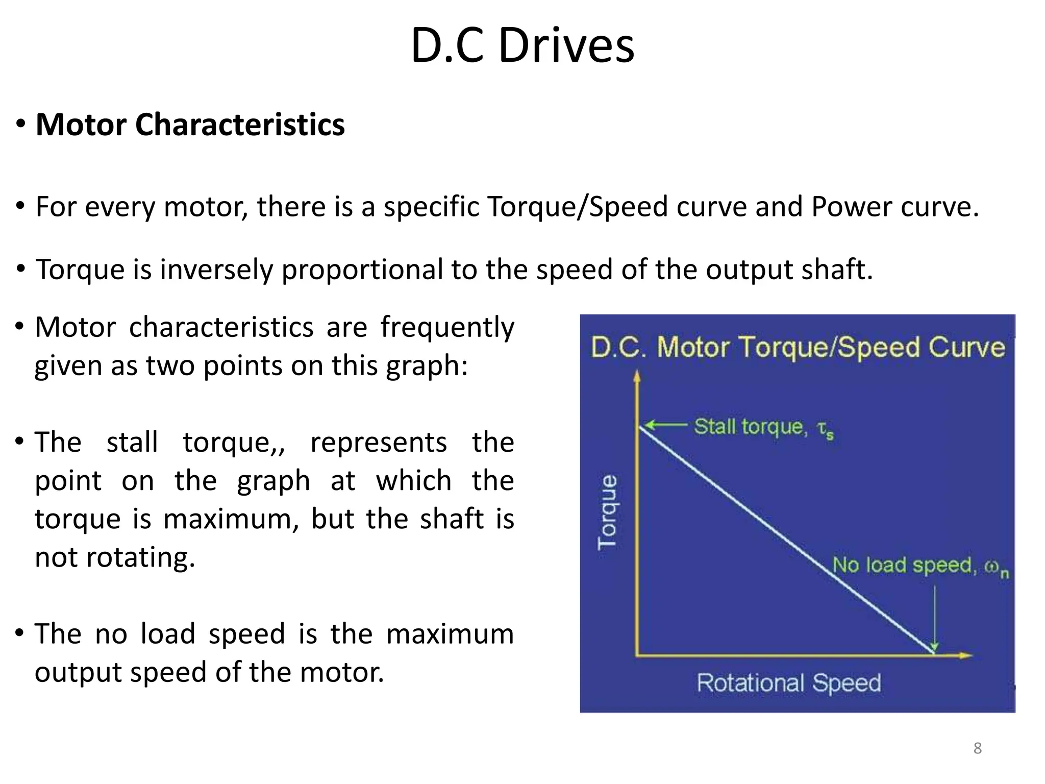
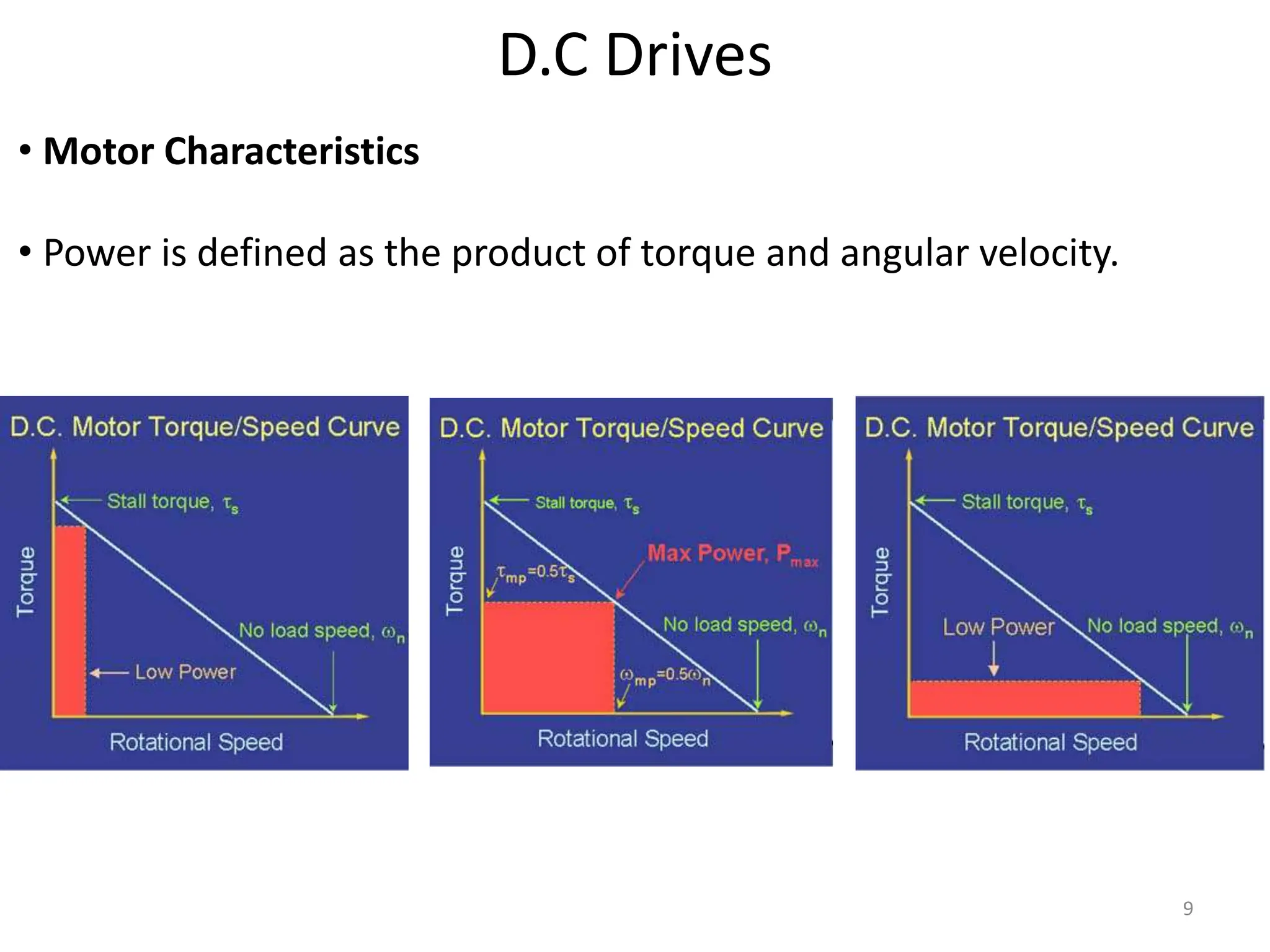
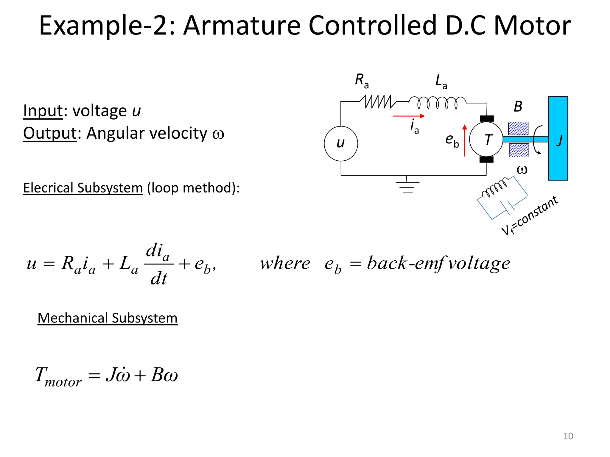
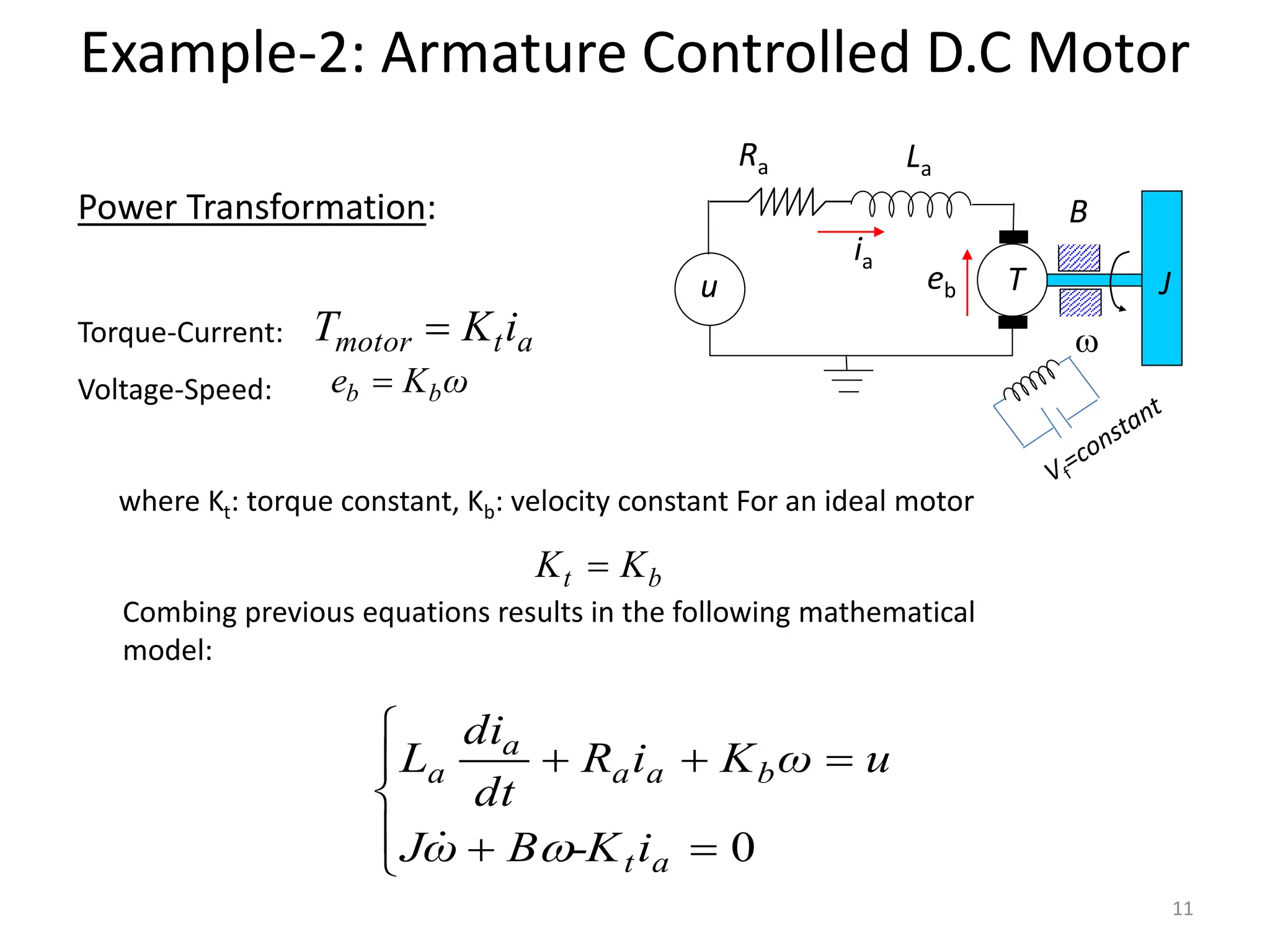
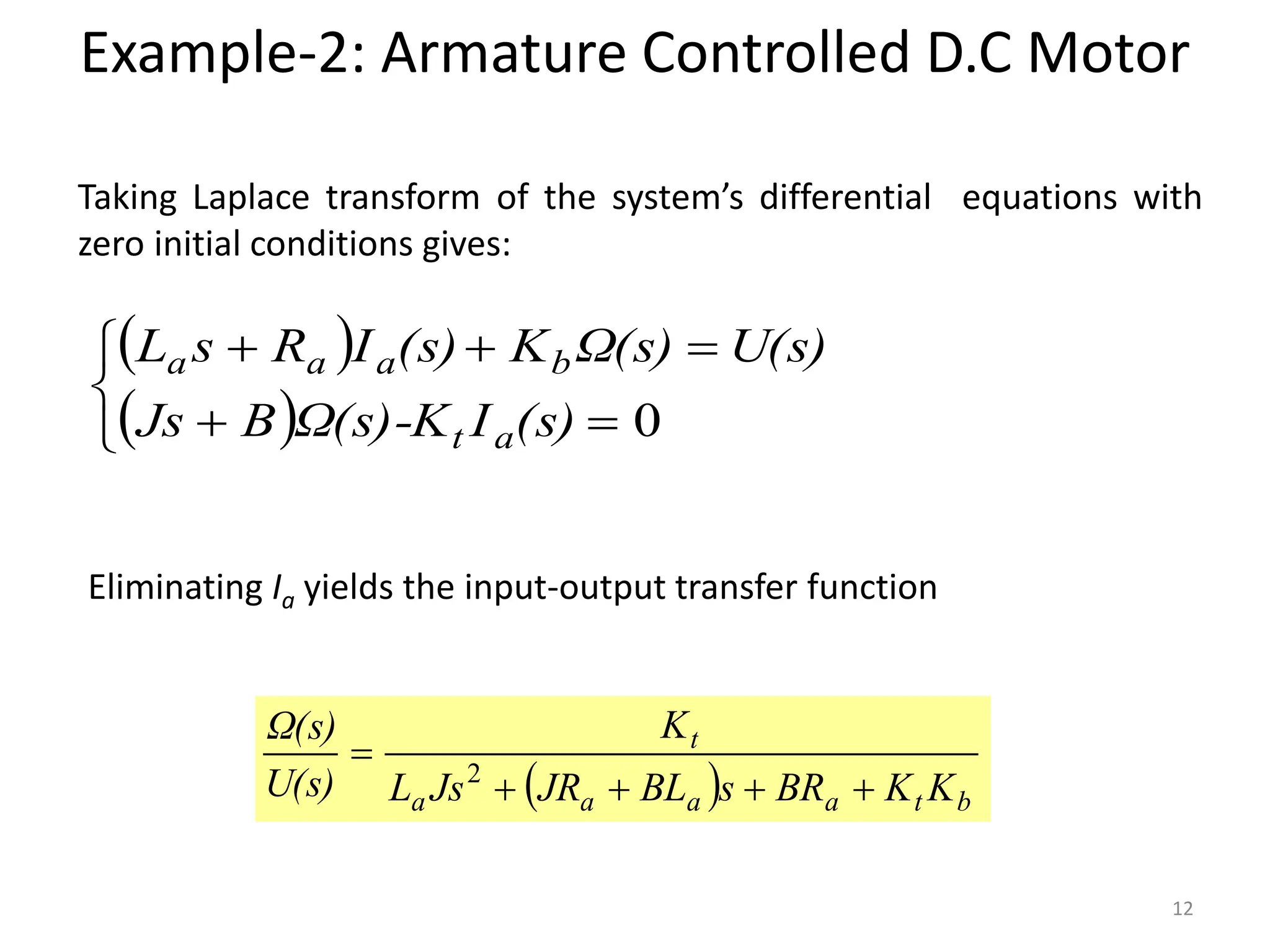
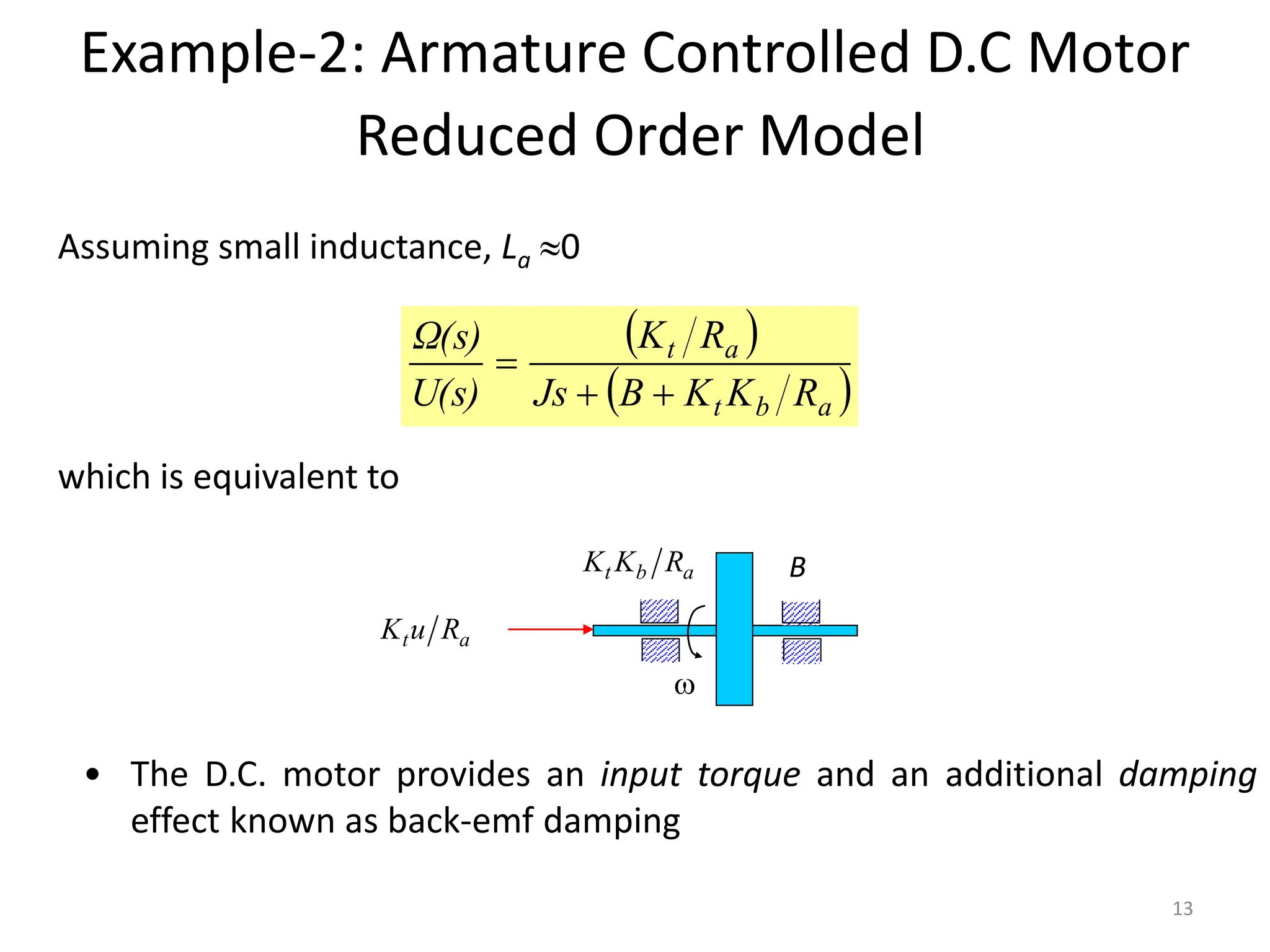
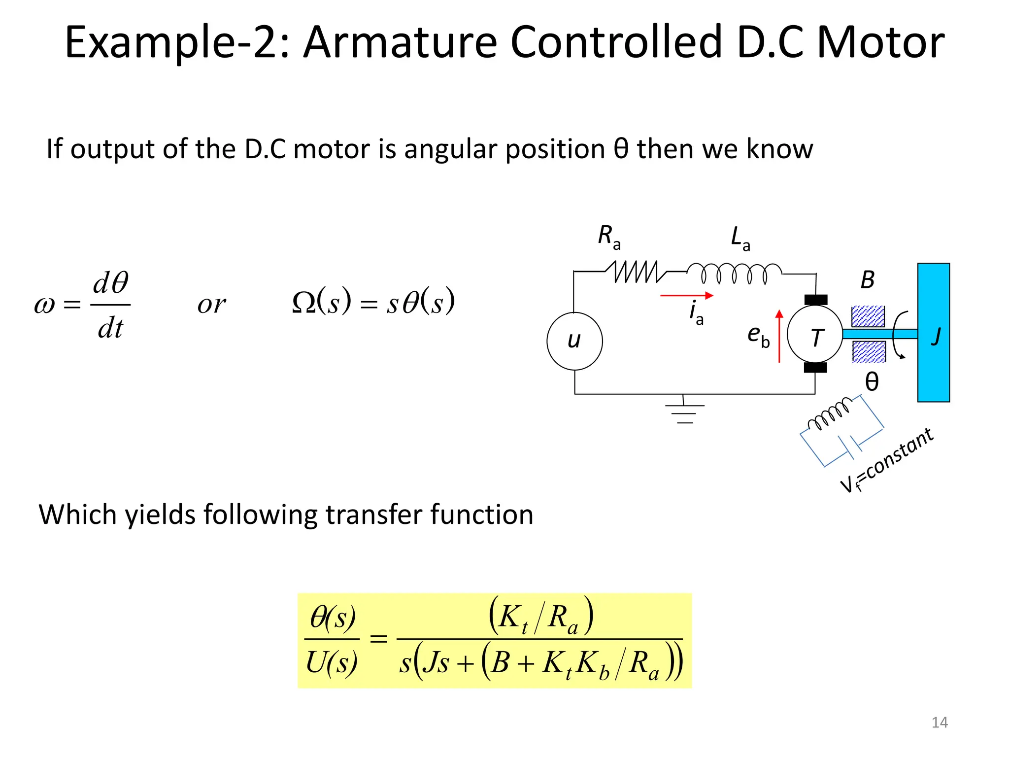
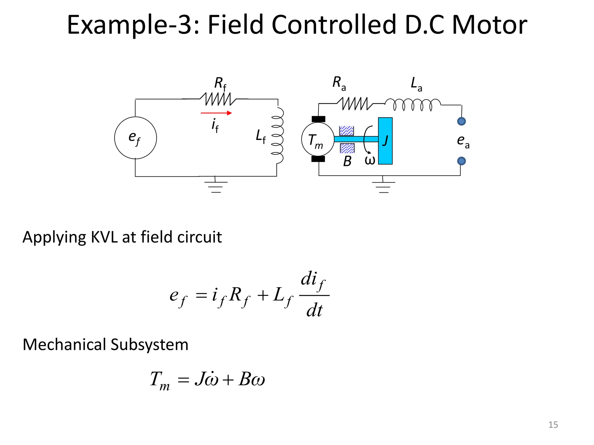
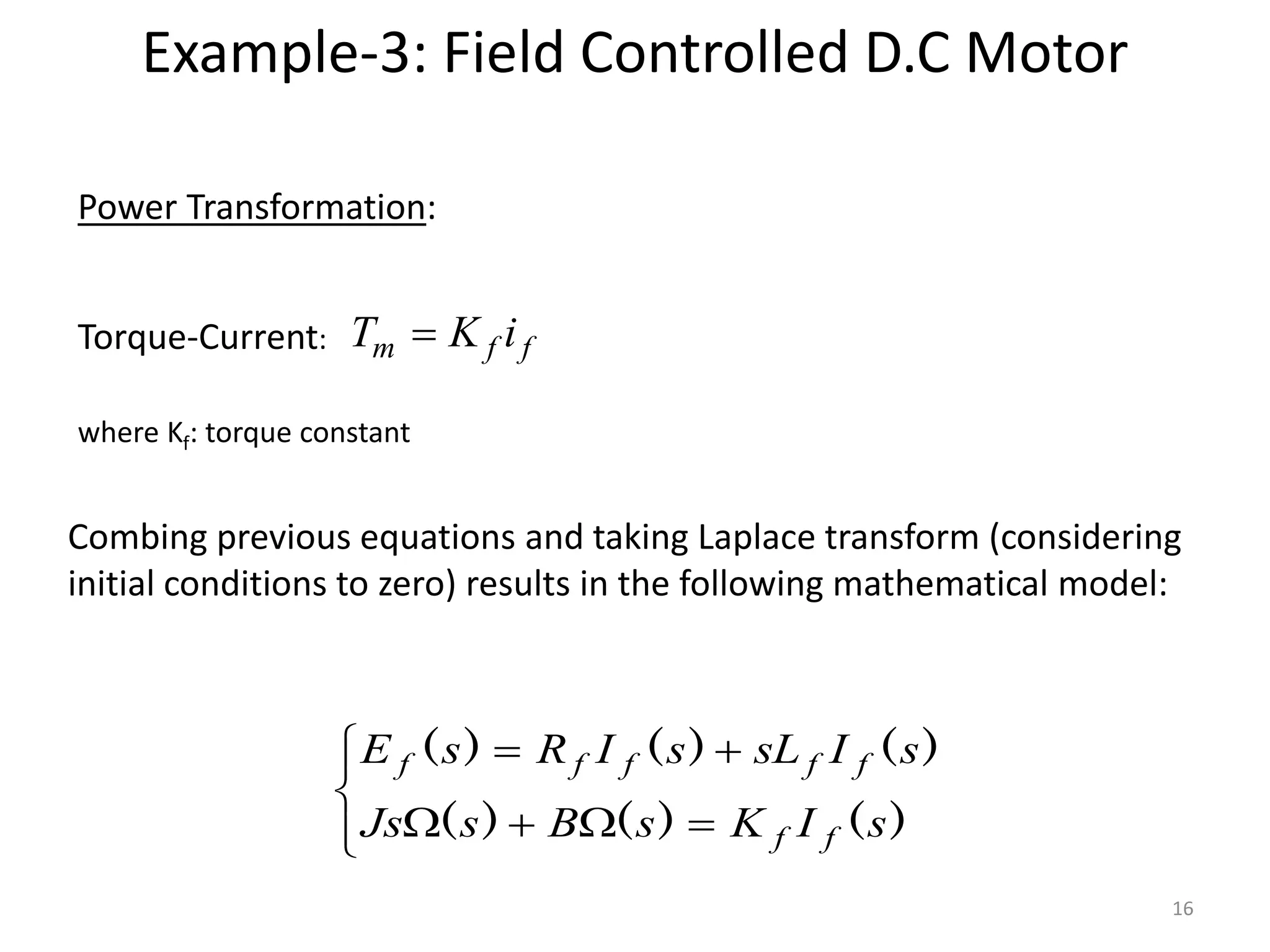
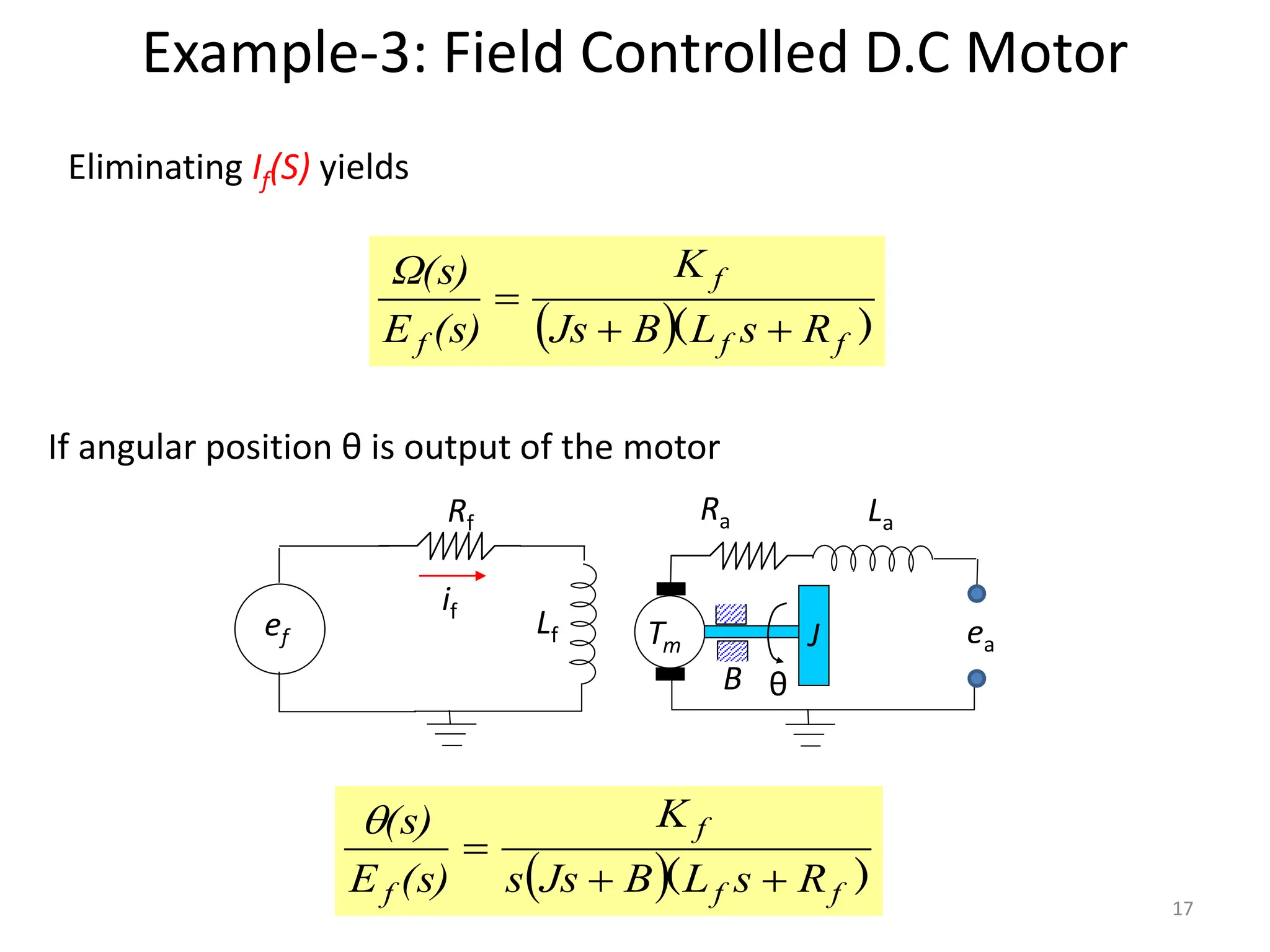
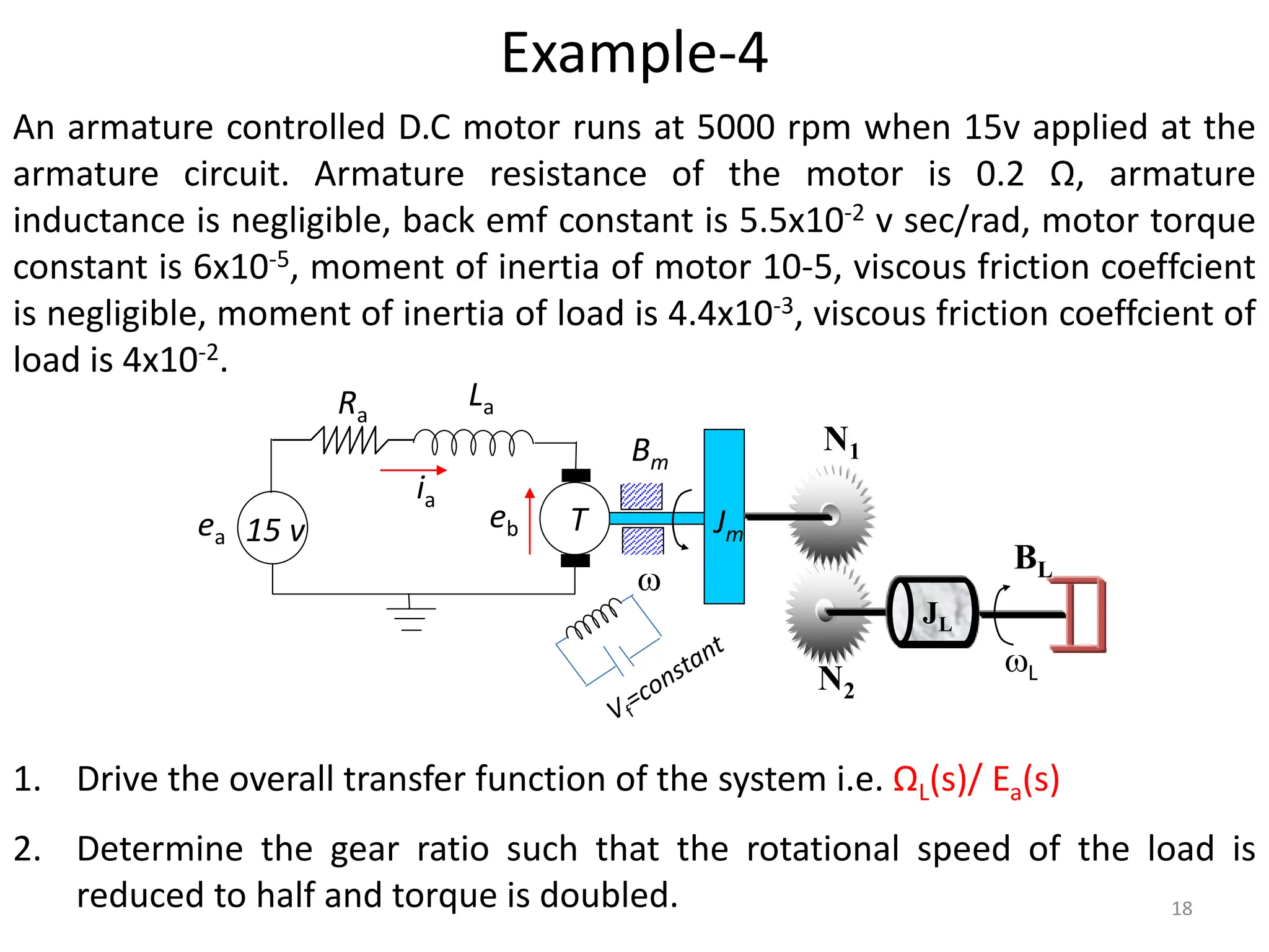
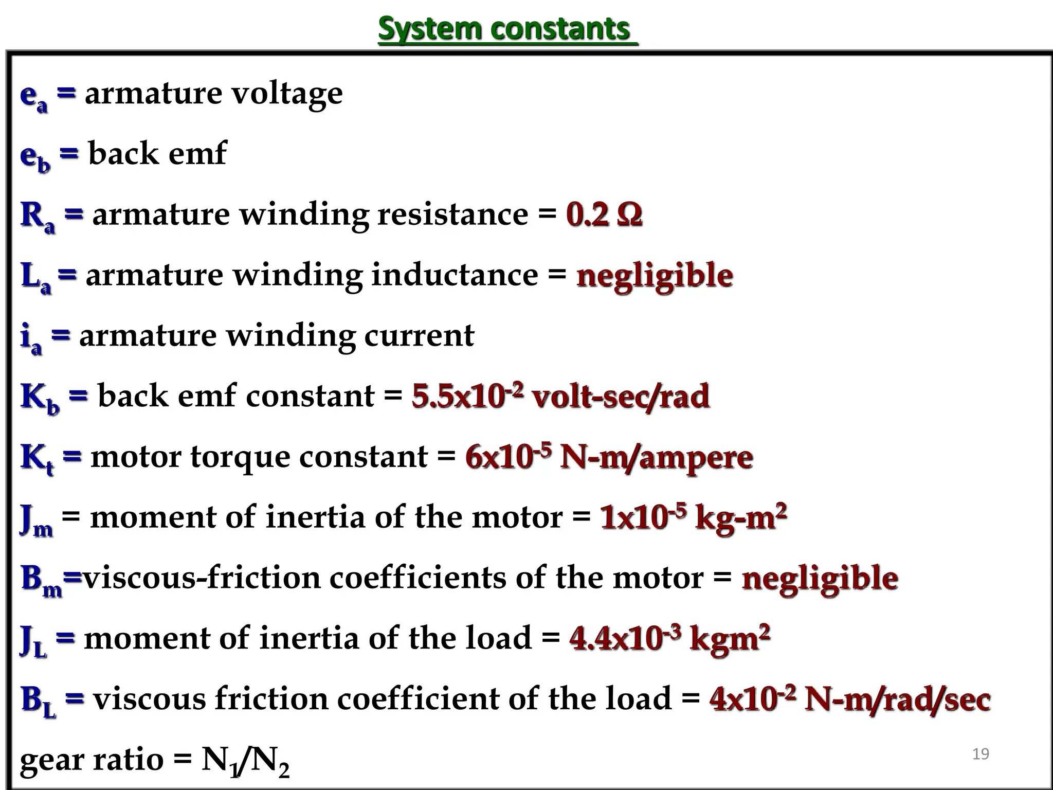
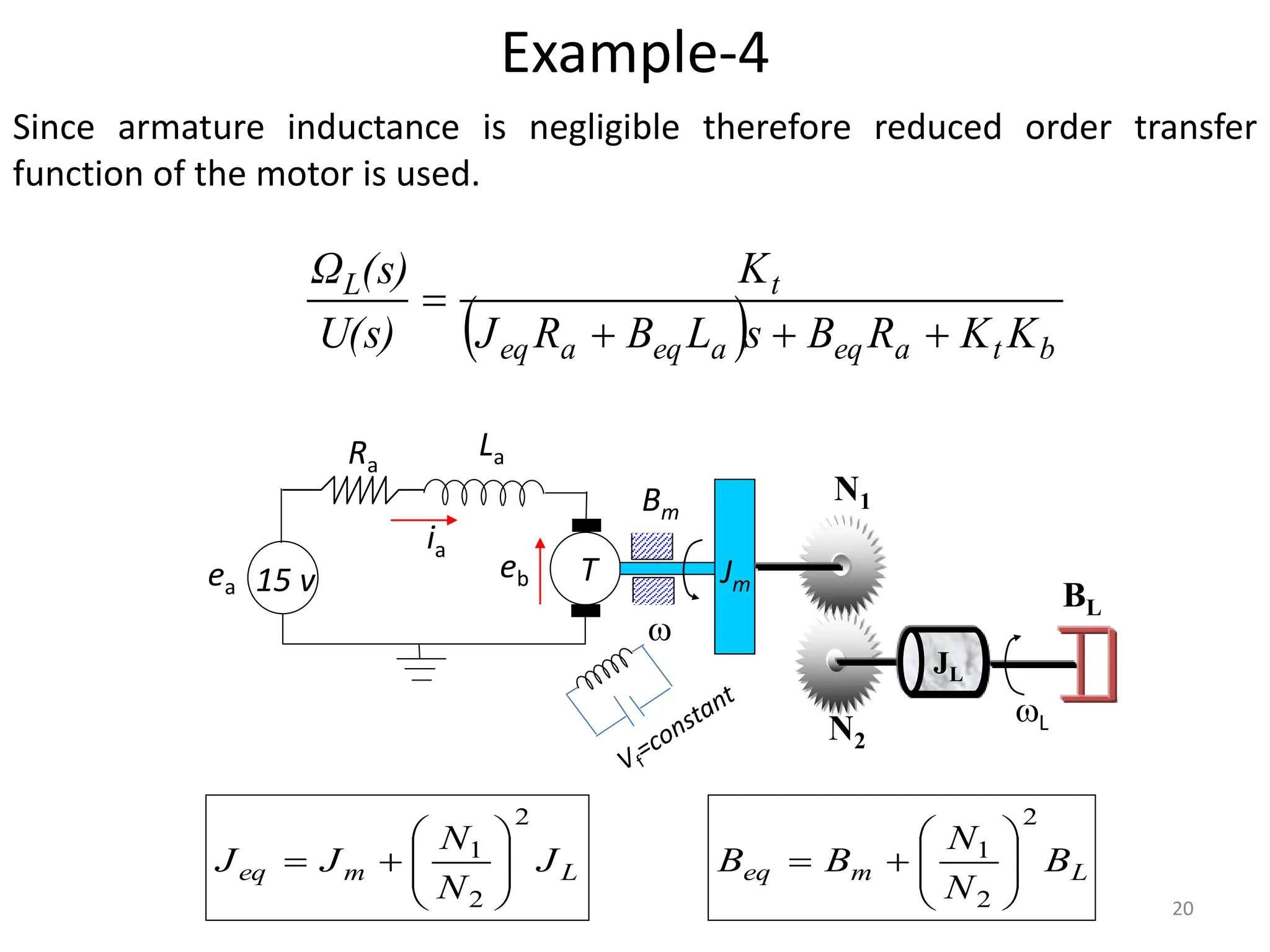
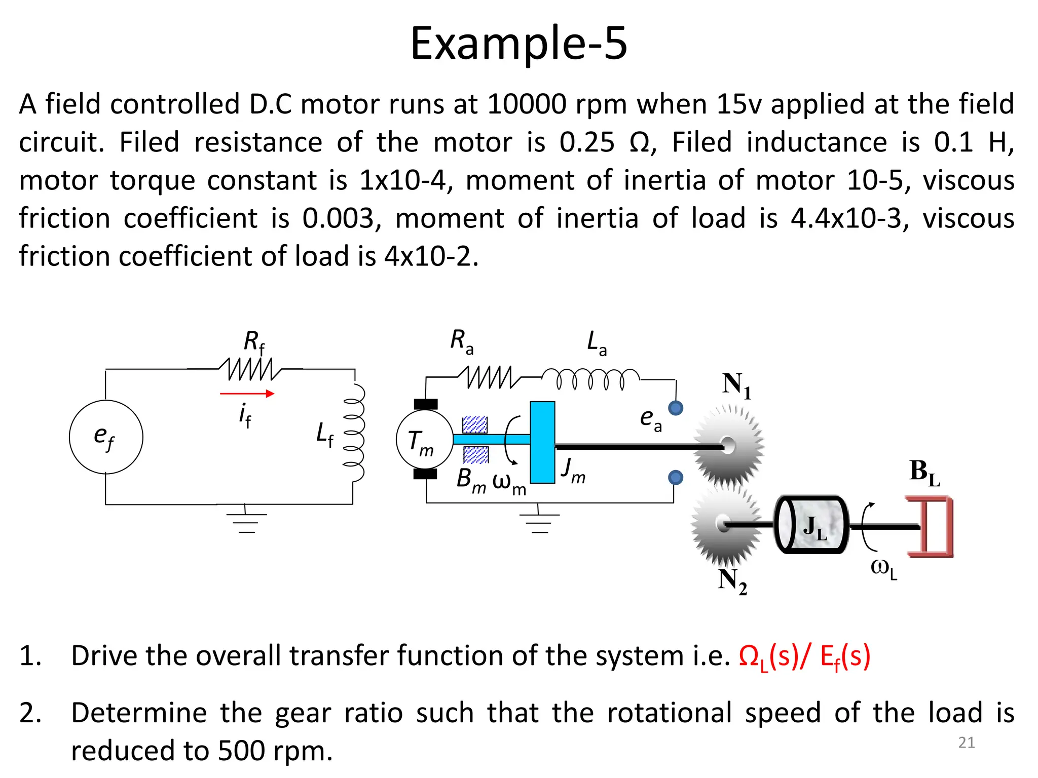
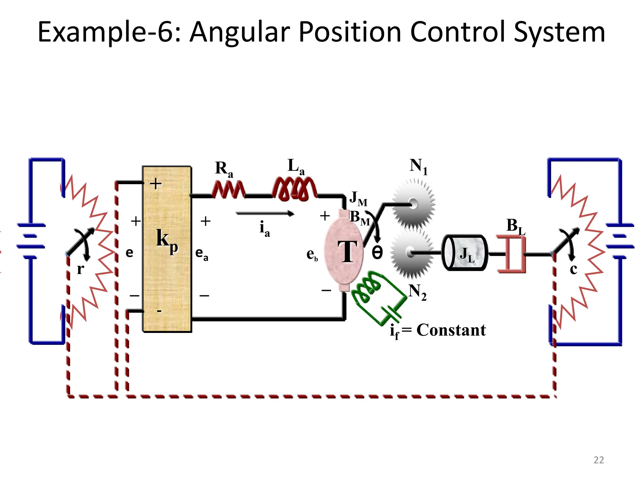
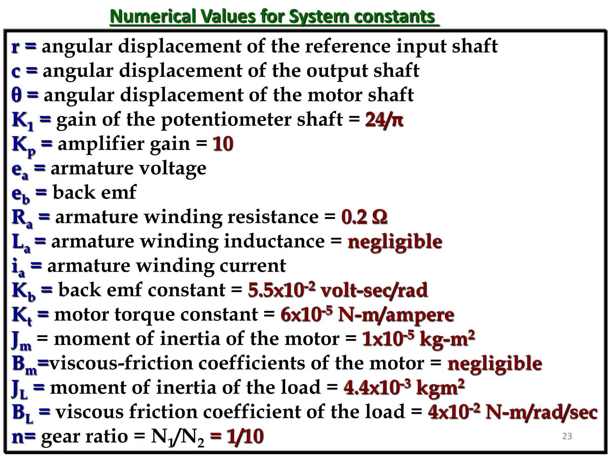
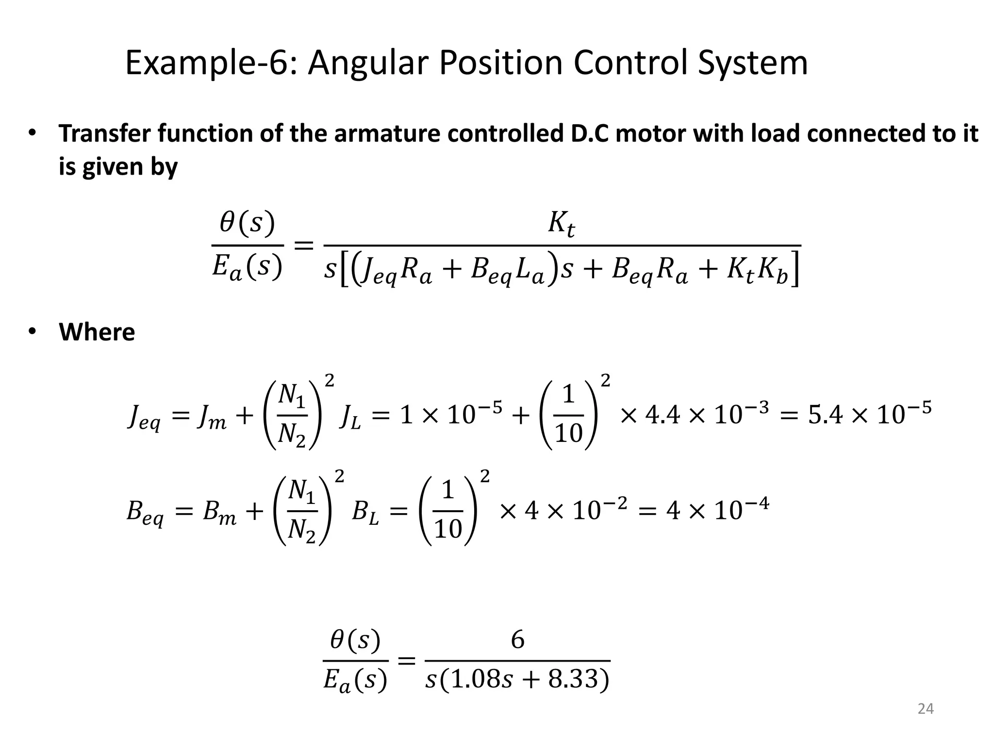
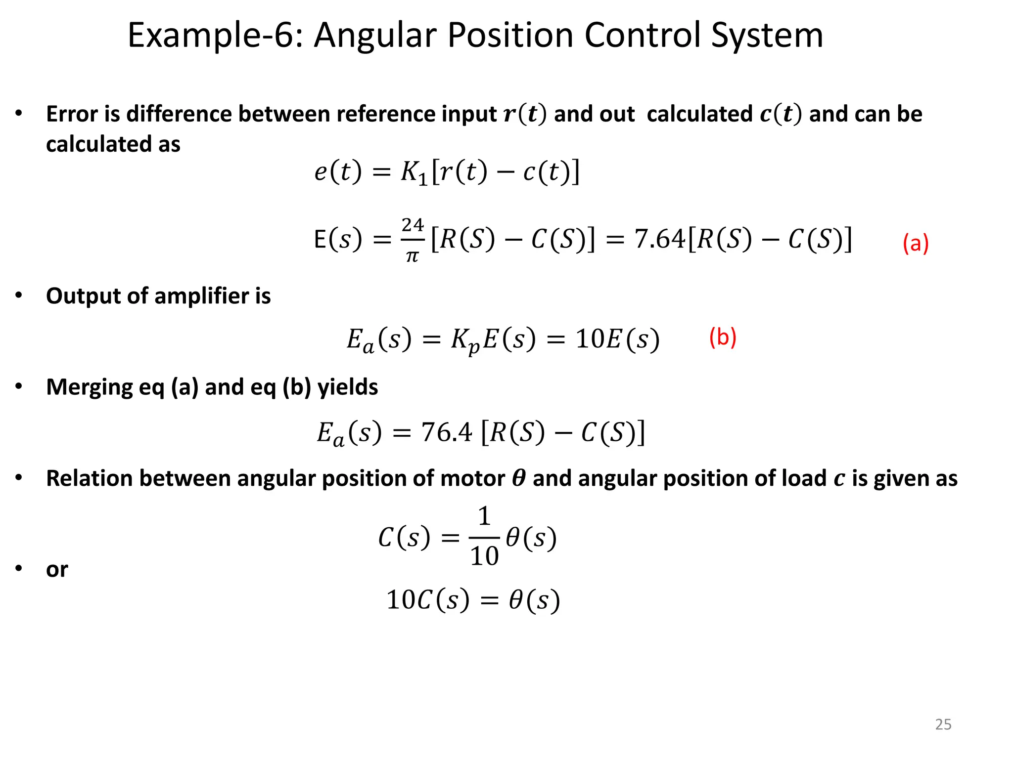
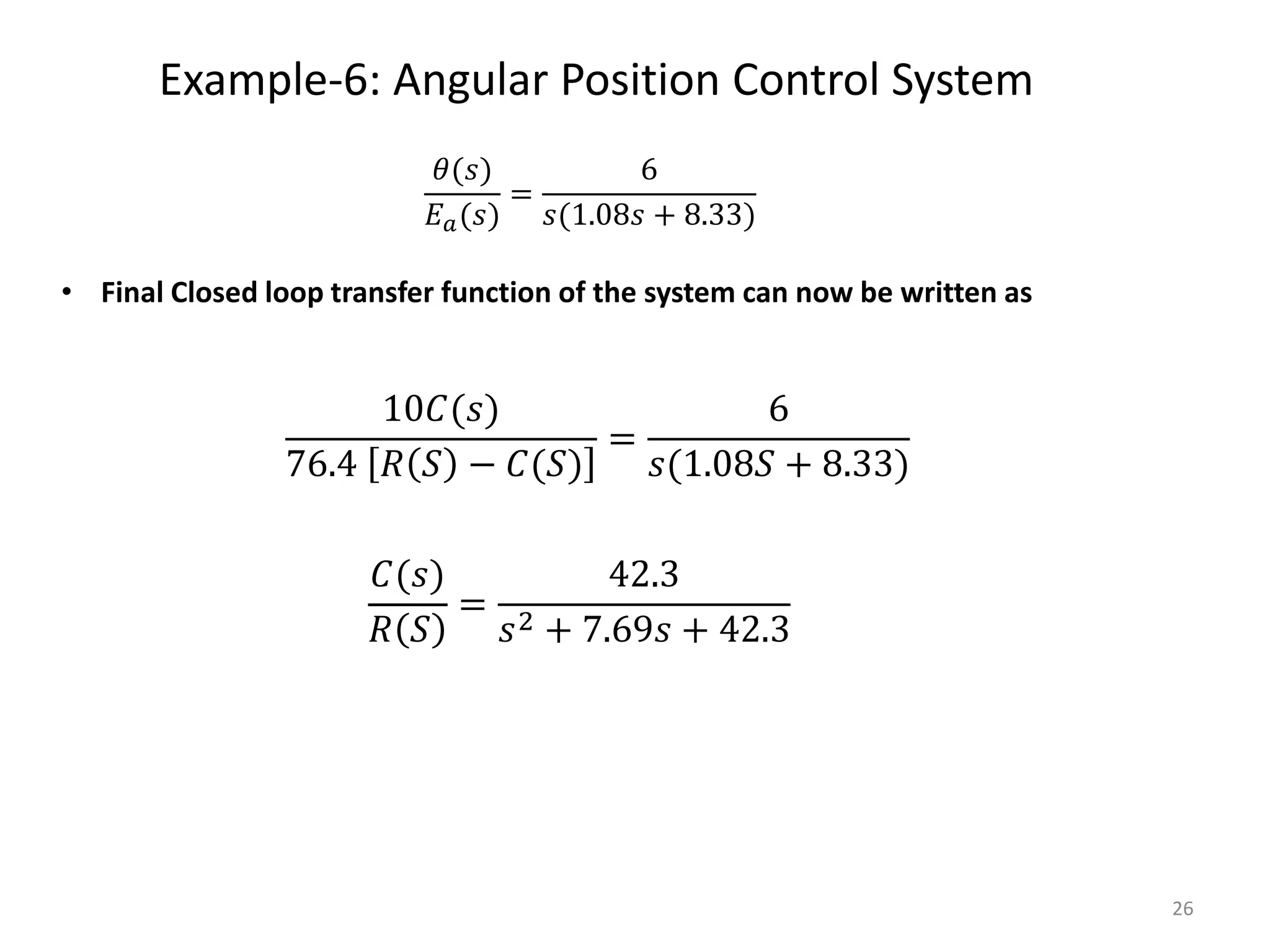
Control Systems (CS)
Dr. Imtiaz Hussain
Associate Professor
Mehran University of Engineering & Technology Jamshoro, Pakistan
email: imtiaz.hussain@faculty.muet.edu.pk
URL :http://imtiazhussainkalwar.weebly.com/
Lecture-6-7
Mathematical Modeling of Electromechanical Systems
1
Electromechanical Systems
• Electromechanics combines electrical and mechanical
processes.
• Devices which carry out electrical operations by using
moving parts are known as electromechanical.
– Relays
– Solenoids
– Electric Motors
– Electric Generators
– Switches and e.t.c
2
Example-1: Potentiometer
3
Example-1: Potentiometer
4
• The resistance between the wiper
(slider) and "A" is labeled R1, the
resistance between the wiper and "B" is
labeled R2.
• The total resistance between "A" and "B"
is constant, R1+R2=Rtot.
• If the potentiometer is turned to the
extreme counterclockwise position such
that the wiper is touching "A" we will call
this θ=0; in this position R1=0 and
R2=Rtot.
• If the wiper is in the extreme clockwise
position such that it is touching "B" we
will call this θ=θmax; in this position
R1=Rtot and R2=0.
Example-1: Potentiometer
5
• R1 and R2 vary linearly with θ between the
two extremes:
tot
R
R
max



1
tot
R
R
max
max


 

2
Example-1: Potentiometer
6
• Potentiometer can be used to sense
angular position, consider the circuit
of figure-1.
• Using the voltage divider principle we
can write:
in
tot
in
out e
R
R
e
R
R
R
e 1
2
1
1



in
out e
e
max



Figure-1
7
D.C Drives
• Speed control can be achieved using
DC drives in a number of ways.
• Variable Voltage can be applied to the
armature terminals of the DC motor .
• Another method is to vary the flux per
pole of the motor.
• The first method involve adjusting the
motor’s armature while the latter
method involves adjusting the motor
field. These methods are referred to as
“armature control” and “field control.”
8
D.C Drives
• Motor Characteristics
• For every motor, there is a specific Torque/Speed curve and Power curve.
• Torque is inversely proportional to the speed of the output shaft.
• Motor characteristics are frequently
given as two points on this graph:
• The stall torque,, represents the
point on the graph at which the
torque is maximum, but the shaft is
not rotating.
• The no load speed is the maximum
output speed of the motor.
9
D.C Drives
• Motor Characteristics
• Power is defined as the product of torque and angular velocity.
oltage
back-emf v
where e
,
e
dt
di
L
i
R
u b
b
a
a
a
a 



Mechanical Subsystem
Bω
ω
J
Tmotor 
 
Input: voltage u
Output: Angular velocity 
Elecrical Subsystem (loop method):
Example-2: Armature Controlled D.C Motor
u
ia
T
Ra La
J

B
eb
10
Torque-Current:
Voltage-Speed:
a
t
motor i
K
T 
Combing previous equations results in the following mathematical
model:
Power Transformation:
ω
K
e b
b 










0
a
t
b
a
a
a
a
i
-K
B
ω
J
u
ω
K
i
R
dt
di
L


where Kt: torque constant, Kb: velocity constant For an ideal motor
b
t K
K 
Example-2: Armature Controlled D.C Motor
u
ia
T
Ra La
J

B
eb
11
Taking Laplace transform of the system’s differential equations with
zero initial conditions gives:
Eliminating Ia yields the input-output transfer function
  b
t
a
a
a
a
t
K
K
BR
s
BL
JR
Js
L
K
U(s)
Ω(s)




 2
 
 








0
(s)
I
Ω(s)-K
B
Js
U(s)
Ω(s)
K
(s)
I
R
s
L
a
t
b
a
a
a
Example-2: Armature Controlled D.C Motor
12
Reduced Order Model
Assuming small inductance, La 0
 
 
a
b
t
a
t
R
K
K
B
Js
R
K
U(s)
Ω(s)



which is equivalent to

a
t R
u
K
B
a
b
t R
K
K
• The D.C. motor provides an input torque and an additional damping
effect known as back-emf damping
Example-2: Armature Controlled D.C Motor
13
If output of the D.C motor is angular position θ then we know
 
 
 
a
b
t
a
t
R
K
K
B
Js
s
R
K
U(s)
(s)




Which yields following transfer function
Example-2: Armature Controlled D.C Motor
)
(
)
( s
s
s
or
dt
d


 


u
ia
T
Ra La
J
θ
B
eb
14
Applying KVL at field circuit
Example-3: Field Controlled D.C Motor
if
Tm
Rf
Lf J
ω
B
Ra La
ea
ef
dt
di
L
R
i
e
f
f
f
f
f 

Mechanical Subsystem
Bω
ω
J
Tm 
 
15
Torque-Current: f
f
m i
K
T 
Combing previous equations and taking Laplace transform (considering
initial conditions to zero) results in the following mathematical model:
Power Transformation:











)
(
)
(
)
(
)
(
)
(
)
(
s
I
K
s
B
s
Js
s
I
sL
s
I
R
s
E
f
f
f
f
f
f
f
where Kf: torque constant
Example-3: Field Controlled D.C Motor
16
If angular position θ is output of the motor
Eliminating If(S) yields
Example-3: Field Controlled D.C Motor
  )
( f
f
f
f R
s
L
B
Js
K
(s)
E
Ω(s)



if
Tm
Rf
Lf J
θ
B
Ra La
ea
ef
  )
( f
f
f
f R
s
L
B
Js
s
K
(s)
E
(s)




17
An armature controlled D.C motor runs at 5000 rpm when 15v applied at the
armature circuit. Armature resistance of the motor is 0.2 Ω, armature
inductance is negligible, back emf constant is 5.5x10⁻² v sec/rad, motor torque
constant is 6x10⁻⁵, moment of inertia of motor 10-5, viscous friction coeffcient
is negligible, moment of inertia of load is 4.4x10⁻³, viscous friction coeffcient of
load is 4x10⁻².
1. Drive the overall transfer function of the system i.e. ΩL(s)/ Ea(s)
2. Determine the gear ratio such that the rotational speed of the load is
reduced to half and torque is doubled.
Example-4
15 v
ia
T
Ra
La
Jm

Bm
eb
JL
N1
N2
BL
L
ea
18
System constants
ea = armature voltage
eb = back emf
Ra = armature winding resistance = 0.2 Ω
La = armature winding inductance = negligible
ia = armature winding current
Kb = back emf constant = 5.5x10⁻² volt-sec/rad
Kt = motor torque constant = 6x10⁻⁵ N-m/ampere
Jm = moment of inertia of the motor = 1x10⁻⁵ kg-m2
Bm=viscous-friction coefficients of the motor = negligible
JL = moment of inertia of the load = 4.4x10⁻³ kgm2
BL = viscous friction coefficient of the load = 4x10⁻² N-m/rad/sec
gear ratio = N1/N2
19
Since armature inductance is negligible therefore reduced order transfer
function of the motor is used.
Example-4
15 v
ia
T
Ra
La
Jm

Bm
eb
JL
N1
N2
BL
L
ea
  b
t
a
eq
a
eq
a
eq
t
L
K
K
R
B
s
L
B
R
J
K
U(s)
(s)
Ω




L
m
eq J
N
N
J
J
2
2
1









 L
m
eq B
N
N
B
B
2
2
1










20
A field controlled D.C motor runs at 10000 rpm when 15v applied at the field
circuit. Filed resistance of the motor is 0.25 Ω, Filed inductance is 0.1 H,
motor torque constant is 1x10⁻⁴, moment of inertia of motor 10-5, viscous
friction coefficient is 0.003, moment of inertia of load is 4.4x10⁻³, viscous
friction coefficient of load is 4x10⁻².
1. Drive the overall transfer function of the system i.e. ΩL(s)/ Ef(s)
2. Determine the gear ratio such that the rotational speed of the load is
reduced to 500 rpm.
Example-5
if
Tm
Rf
Lf
Jm
ωm
Bm
Ra La
ea
ef
JL
N1
N2
BL
L
21
+
kp
-
JL
_
ia
eb
Ra
La
+
T
r c
ea
_
+
e
_
+
N1
N2
BL
θ
if = Constant
JM
BM
22
Example-6: Angular Position Control System
Numerical Values for System constants
r = angular displacement of the reference input shaft
c = angular displacement of the output shaft
θ = angular displacement of the motor shaft
K1 = gain of the potentiometer shaft = 24/π
Kp = amplifier gain = 10
ea = armature voltage
eb = back emf
Ra = armature winding resistance = 0.2 Ω
La = armature winding inductance = negligible
ia = armature winding current
Kb = back emf constant = 5.5x10⁻² volt-sec/rad
Kt = motor torque constant = 6x10⁻⁵ N-m/ampere
Jm = moment of inertia of the motor = 1x10⁻⁵ kg-m2
Bm=viscous-friction coefficients of the motor = negligible
JL = moment of inertia of the load = 4.4x10⁻³ kgm2
BL = viscous friction coefficient of the load = 4x10⁻² N-m/rad/sec
n= gear ratio = N1/N2 = 1/10 23
Example-6: Angular Position Control System
24
• Transfer function of the armature controlled D.C motor with load connected to it
is given by
• Where
𝐽𝑒𝑞 = 𝐽𝑚 +
𝑁1
𝑁2
2
𝐽𝐿 = 1 × 10⁻⁵
+
1
10
2
× 4.4 × 10−3
= 5.4 × 10⁻⁵
𝐵𝑒𝑞 = 𝐵𝑚 +
𝑁1
𝑁2
2
𝐵𝐿 =
1
10
2
× 4 × 10−2 = 4 × 10⁻⁴
𝜃(𝑠)
𝐸𝑎(𝑠)
=
6
𝑠(1.08𝑠 + 8.33)
𝜃(𝑠)
𝐸𝑎(𝑠)
=
𝐾𝑡
𝑠 𝐽𝑒𝑞𝑅𝑎 + 𝐵𝑒𝑞𝐿𝑎 𝑠 + 𝐵𝑒𝑞𝑅𝑎 + 𝐾𝑡𝐾𝑏
Example-6: Angular Position Control System
25
𝑒 𝑡 = 𝐾1 𝑟 𝑡 − 𝑐(𝑡)
• Error is difference between reference input 𝒓 𝒕 and out calculated 𝒄 𝒕 and can be
calculated as
• Output of amplifier is
• Merging eq (a) and eq (b) yields
• Relation between angular position of motor 𝜽 and angular position of load 𝒄 is given as
• or
E 𝑠 =
24
𝜋
𝑅 𝑆 − 𝐶(𝑆) = 7.64 𝑅 𝑆 − 𝐶(𝑆)
𝐸𝑎 𝑠 = 𝐾𝑝𝐸 𝑠 = 10𝐸(𝑠)
𝐸𝑎 𝑠 = 76.4 𝑅 𝑆 − 𝐶(𝑆)
(a)
(b)
𝐶 𝑠 =
1
10
𝜃(𝑠)
10𝐶 𝑠 = 𝜃(𝑠)
Example-6: Angular Position Control System
26
• Final Closed loop transfer function of the system can now be written as
10𝐶(𝑠)
76.4 𝑅 𝑆 − 𝐶(𝑆)
=
6
𝑠(1.08𝑆 + 8.33)
𝐶(𝑠)
𝑅 𝑆
=
42.3
𝑠2 + 7.69𝑠 + 42.3
𝜃(𝑠)
𝐸𝑎(𝑠)
=
6
𝑠(1.08𝑠 + 8.33)
END OF LECTURES-6-7
To download this lecture visit
http://imtiazhussainkalwar.weebly.com/
27

lecture-6-7_modeling_of__electromechanical_systems.pptx

  • 1.
    Control Systems (CS) Dr.Imtiaz Hussain Associate Professor Mehran University of Engineering & Technology Jamshoro, Pakistan email: imtiaz.hussain@faculty.muet.edu.pk URL :http://imtiazhussainkalwar.weebly.com/ Lecture-6-7 Mathematical Modeling of Electromechanical Systems 1
  • 2.
    Electromechanical Systems • Electromechanicscombines electrical and mechanical processes. • Devices which carry out electrical operations by using moving parts are known as electromechanical. – Relays – Solenoids – Electric Motors – Electric Generators – Switches and e.t.c 2
  • 3.
  • 4.
    Example-1: Potentiometer 4 • Theresistance between the wiper (slider) and "A" is labeled R1, the resistance between the wiper and "B" is labeled R2. • The total resistance between "A" and "B" is constant, R1+R2=Rtot. • If the potentiometer is turned to the extreme counterclockwise position such that the wiper is touching "A" we will call this θ=0; in this position R1=0 and R2=Rtot. • If the wiper is in the extreme clockwise position such that it is touching "B" we will call this θ=θmax; in this position R1=Rtot and R2=0.
  • 5.
    Example-1: Potentiometer 5 • R1and R2 vary linearly with θ between the two extremes: tot R R max    1 tot R R max max      2
  • 6.
    Example-1: Potentiometer 6 • Potentiometercan be used to sense angular position, consider the circuit of figure-1. • Using the voltage divider principle we can write: in tot in out e R R e R R R e 1 2 1 1    in out e e max    Figure-1
  • 7.
    7 D.C Drives • Speedcontrol can be achieved using DC drives in a number of ways. • Variable Voltage can be applied to the armature terminals of the DC motor . • Another method is to vary the flux per pole of the motor. • The first method involve adjusting the motor’s armature while the latter method involves adjusting the motor field. These methods are referred to as “armature control” and “field control.”
  • 8.
    8 D.C Drives • MotorCharacteristics • For every motor, there is a specific Torque/Speed curve and Power curve. • Torque is inversely proportional to the speed of the output shaft. • Motor characteristics are frequently given as two points on this graph: • The stall torque,, represents the point on the graph at which the torque is maximum, but the shaft is not rotating. • The no load speed is the maximum output speed of the motor.
  • 9.
    9 D.C Drives • MotorCharacteristics • Power is defined as the product of torque and angular velocity.
  • 10.
    oltage back-emf v where e , e dt di L i R ub b a a a a     Mechanical Subsystem Bω ω J Tmotor    Input: voltage u Output: Angular velocity  Elecrical Subsystem (loop method): Example-2: Armature Controlled D.C Motor u ia T Ra La J  B eb 10
  • 11.
    Torque-Current: Voltage-Speed: a t motor i K T  Combingprevious equations results in the following mathematical model: Power Transformation: ω K e b b            0 a t b a a a a i -K B ω J u ω K i R dt di L   where Kt: torque constant, Kb: velocity constant For an ideal motor b t K K  Example-2: Armature Controlled D.C Motor u ia T Ra La J  B eb 11
  • 12.
    Taking Laplace transformof the system’s differential equations with zero initial conditions gives: Eliminating Ia yields the input-output transfer function   b t a a a a t K K BR s BL JR Js L K U(s) Ω(s)      2             0 (s) I Ω(s)-K B Js U(s) Ω(s) K (s) I R s L a t b a a a Example-2: Armature Controlled D.C Motor 12
  • 13.
    Reduced Order Model Assumingsmall inductance, La 0     a b t a t R K K B Js R K U(s) Ω(s)    which is equivalent to  a t R u K B a b t R K K • The D.C. motor provides an input torque and an additional damping effect known as back-emf damping Example-2: Armature Controlled D.C Motor 13
  • 14.
    If output ofthe D.C motor is angular position θ then we know       a b t a t R K K B Js s R K U(s) (s)     Which yields following transfer function Example-2: Armature Controlled D.C Motor ) ( ) ( s s s or dt d       u ia T Ra La J θ B eb 14
  • 15.
    Applying KVL atfield circuit Example-3: Field Controlled D.C Motor if Tm Rf Lf J ω B Ra La ea ef dt di L R i e f f f f f   Mechanical Subsystem Bω ω J Tm    15
  • 16.
    Torque-Current: f f m i K T Combing previous equations and taking Laplace transform (considering initial conditions to zero) results in the following mathematical model: Power Transformation:            ) ( ) ( ) ( ) ( ) ( ) ( s I K s B s Js s I sL s I R s E f f f f f f f where Kf: torque constant Example-3: Field Controlled D.C Motor 16
  • 17.
    If angular positionθ is output of the motor Eliminating If(S) yields Example-3: Field Controlled D.C Motor   ) ( f f f f R s L B Js K (s) E Ω(s)    if Tm Rf Lf J θ B Ra La ea ef   ) ( f f f f R s L B Js s K (s) E (s)     17
  • 18.
    An armature controlledD.C motor runs at 5000 rpm when 15v applied at the armature circuit. Armature resistance of the motor is 0.2 Ω, armature inductance is negligible, back emf constant is 5.5x10⁻² v sec/rad, motor torque constant is 6x10⁻⁵, moment of inertia of motor 10-5, viscous friction coeffcient is negligible, moment of inertia of load is 4.4x10⁻³, viscous friction coeffcient of load is 4x10⁻². 1. Drive the overall transfer function of the system i.e. ΩL(s)/ Ea(s) 2. Determine the gear ratio such that the rotational speed of the load is reduced to half and torque is doubled. Example-4 15 v ia T Ra La Jm  Bm eb JL N1 N2 BL L ea 18
  • 19.
    System constants ea =armature voltage eb = back emf Ra = armature winding resistance = 0.2 Ω La = armature winding inductance = negligible ia = armature winding current Kb = back emf constant = 5.5x10⁻² volt-sec/rad Kt = motor torque constant = 6x10⁻⁵ N-m/ampere Jm = moment of inertia of the motor = 1x10⁻⁵ kg-m2 Bm=viscous-friction coefficients of the motor = negligible JL = moment of inertia of the load = 4.4x10⁻³ kgm2 BL = viscous friction coefficient of the load = 4x10⁻² N-m/rad/sec gear ratio = N1/N2 19
  • 20.
    Since armature inductanceis negligible therefore reduced order transfer function of the motor is used. Example-4 15 v ia T Ra La Jm  Bm eb JL N1 N2 BL L ea   b t a eq a eq a eq t L K K R B s L B R J K U(s) (s) Ω     L m eq J N N J J 2 2 1           L m eq B N N B B 2 2 1           20
  • 21.
    A field controlledD.C motor runs at 10000 rpm when 15v applied at the field circuit. Filed resistance of the motor is 0.25 Ω, Filed inductance is 0.1 H, motor torque constant is 1x10⁻⁴, moment of inertia of motor 10-5, viscous friction coefficient is 0.003, moment of inertia of load is 4.4x10⁻³, viscous friction coefficient of load is 4x10⁻². 1. Drive the overall transfer function of the system i.e. ΩL(s)/ Ef(s) 2. Determine the gear ratio such that the rotational speed of the load is reduced to 500 rpm. Example-5 if Tm Rf Lf Jm ωm Bm Ra La ea ef JL N1 N2 BL L 21
  • 22.
    + kp - JL _ ia eb Ra La + T r c ea _ + e _ + N1 N2 BL θ if =Constant JM BM 22 Example-6: Angular Position Control System
  • 23.
    Numerical Values forSystem constants r = angular displacement of the reference input shaft c = angular displacement of the output shaft θ = angular displacement of the motor shaft K1 = gain of the potentiometer shaft = 24/π Kp = amplifier gain = 10 ea = armature voltage eb = back emf Ra = armature winding resistance = 0.2 Ω La = armature winding inductance = negligible ia = armature winding current Kb = back emf constant = 5.5x10⁻² volt-sec/rad Kt = motor torque constant = 6x10⁻⁵ N-m/ampere Jm = moment of inertia of the motor = 1x10⁻⁵ kg-m2 Bm=viscous-friction coefficients of the motor = negligible JL = moment of inertia of the load = 4.4x10⁻³ kgm2 BL = viscous friction coefficient of the load = 4x10⁻² N-m/rad/sec n= gear ratio = N1/N2 = 1/10 23
  • 24.
    Example-6: Angular PositionControl System 24 • Transfer function of the armature controlled D.C motor with load connected to it is given by • Where 𝐽𝑒𝑞 = 𝐽𝑚 + 𝑁1 𝑁2 2 𝐽𝐿 = 1 × 10⁻⁵ + 1 10 2 × 4.4 × 10−3 = 5.4 × 10⁻⁵ 𝐵𝑒𝑞 = 𝐵𝑚 + 𝑁1 𝑁2 2 𝐵𝐿 = 1 10 2 × 4 × 10−2 = 4 × 10⁻⁴ 𝜃(𝑠) 𝐸𝑎(𝑠) = 6 𝑠(1.08𝑠 + 8.33) 𝜃(𝑠) 𝐸𝑎(𝑠) = 𝐾𝑡 𝑠 𝐽𝑒𝑞𝑅𝑎 + 𝐵𝑒𝑞𝐿𝑎 𝑠 + 𝐵𝑒𝑞𝑅𝑎 + 𝐾𝑡𝐾𝑏
  • 25.
    Example-6: Angular PositionControl System 25 𝑒 𝑡 = 𝐾1 𝑟 𝑡 − 𝑐(𝑡) • Error is difference between reference input 𝒓 𝒕 and out calculated 𝒄 𝒕 and can be calculated as • Output of amplifier is • Merging eq (a) and eq (b) yields • Relation between angular position of motor 𝜽 and angular position of load 𝒄 is given as • or E 𝑠 = 24 𝜋 𝑅 𝑆 − 𝐶(𝑆) = 7.64 𝑅 𝑆 − 𝐶(𝑆) 𝐸𝑎 𝑠 = 𝐾𝑝𝐸 𝑠 = 10𝐸(𝑠) 𝐸𝑎 𝑠 = 76.4 𝑅 𝑆 − 𝐶(𝑆) (a) (b) 𝐶 𝑠 = 1 10 𝜃(𝑠) 10𝐶 𝑠 = 𝜃(𝑠)
  • 26.
    Example-6: Angular PositionControl System 26 • Final Closed loop transfer function of the system can now be written as 10𝐶(𝑠) 76.4 𝑅 𝑆 − 𝐶(𝑆) = 6 𝑠(1.08𝑆 + 8.33) 𝐶(𝑠) 𝑅 𝑆 = 42.3 𝑠2 + 7.69𝑠 + 42.3 𝜃(𝑠) 𝐸𝑎(𝑠) = 6 𝑠(1.08𝑠 + 8.33)
  • 27.
    END OF LECTURES-6-7 Todownload this lecture visit http://imtiazhussainkalwar.weebly.com/ 27