This document discusses the characteristics and performance of power transmission lines. It covers the following key points:
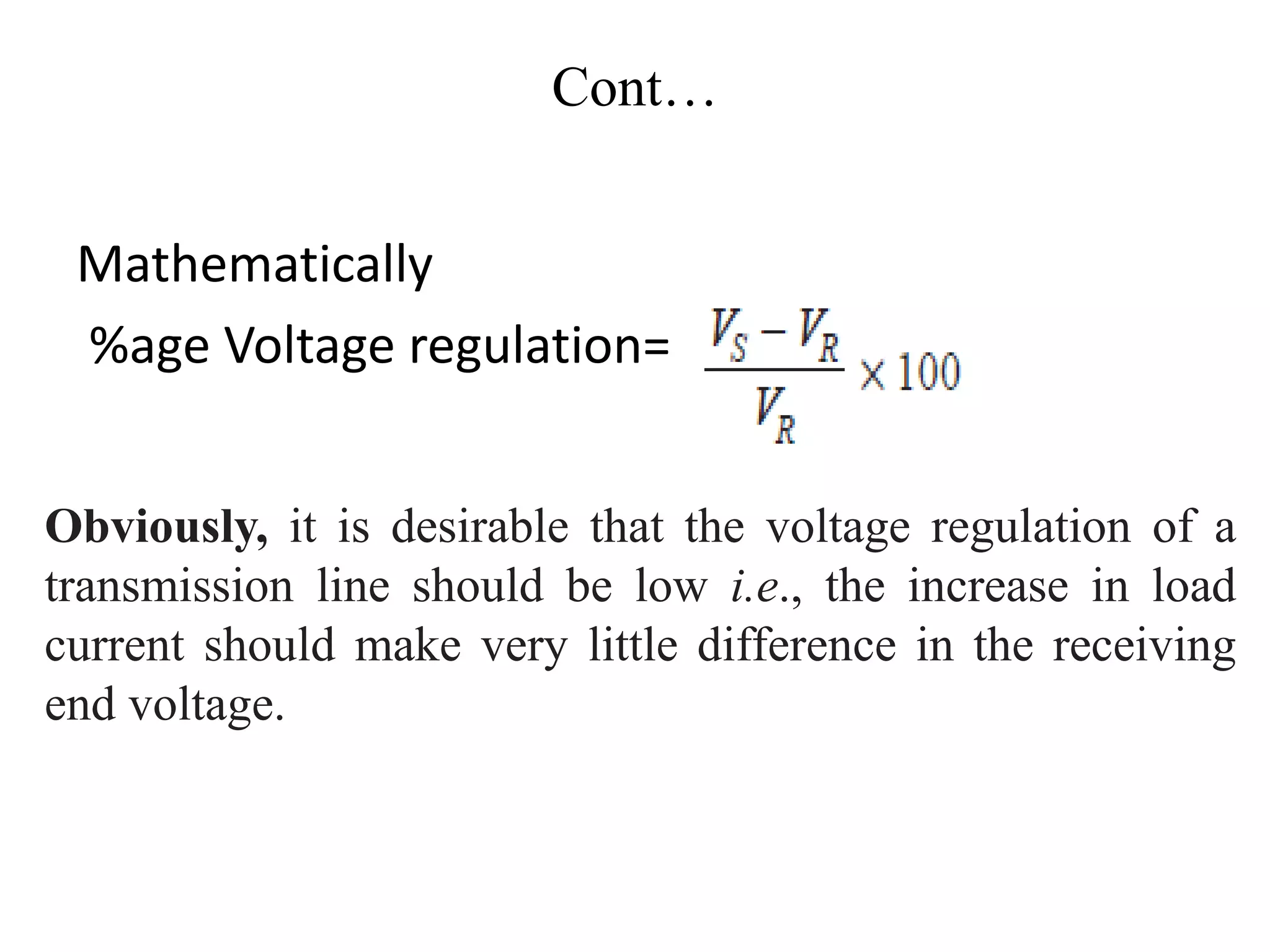
- The design and operation of transmission lines considers voltage drop, line losses, and transmission efficiency, which depend on the line constants R, L, and C.
- Transmission lines are classified as short, medium, or long depending on their length and voltage level. Different methods are used to calculate performance based on how capacitance effects are handled.
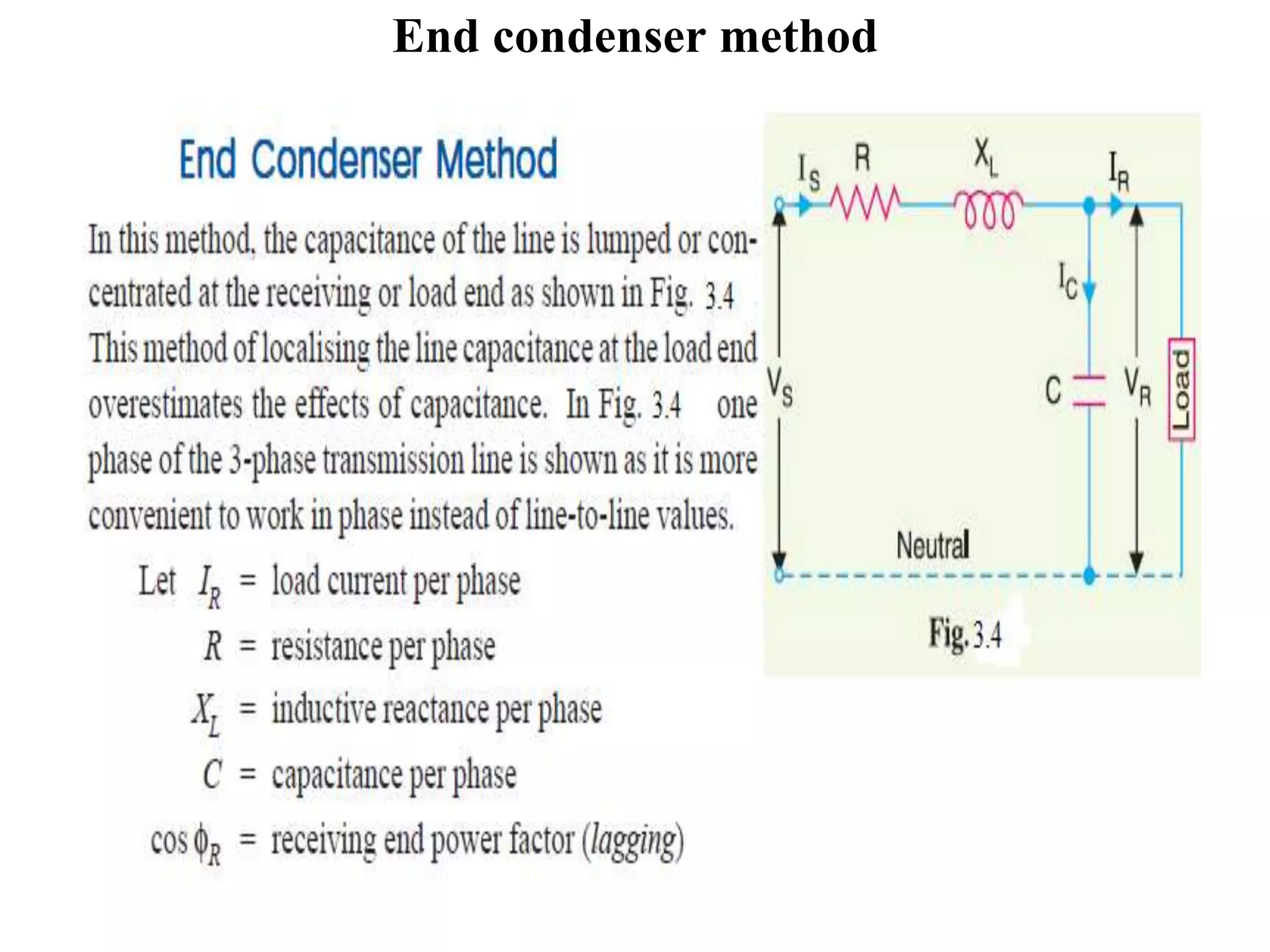
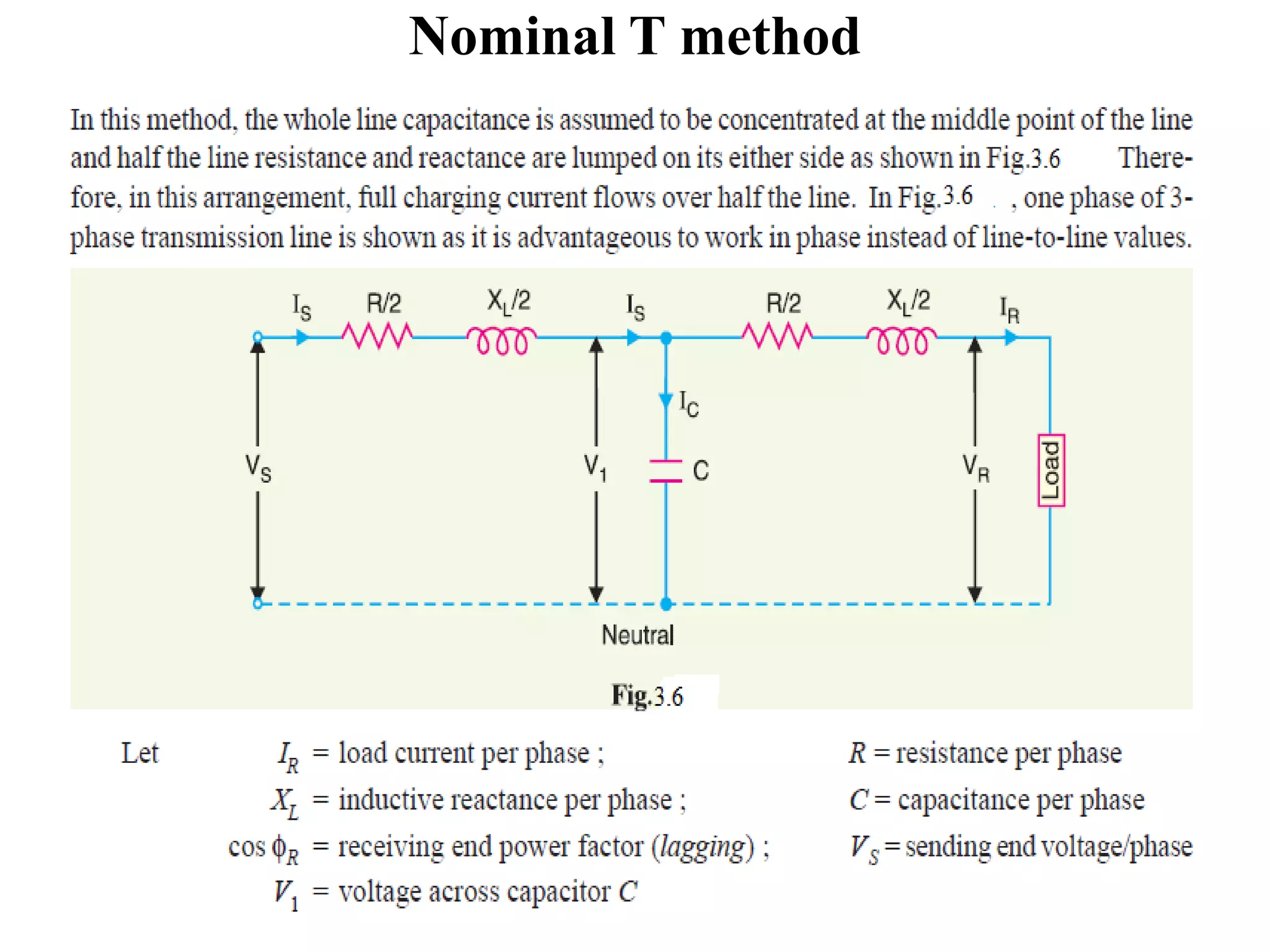
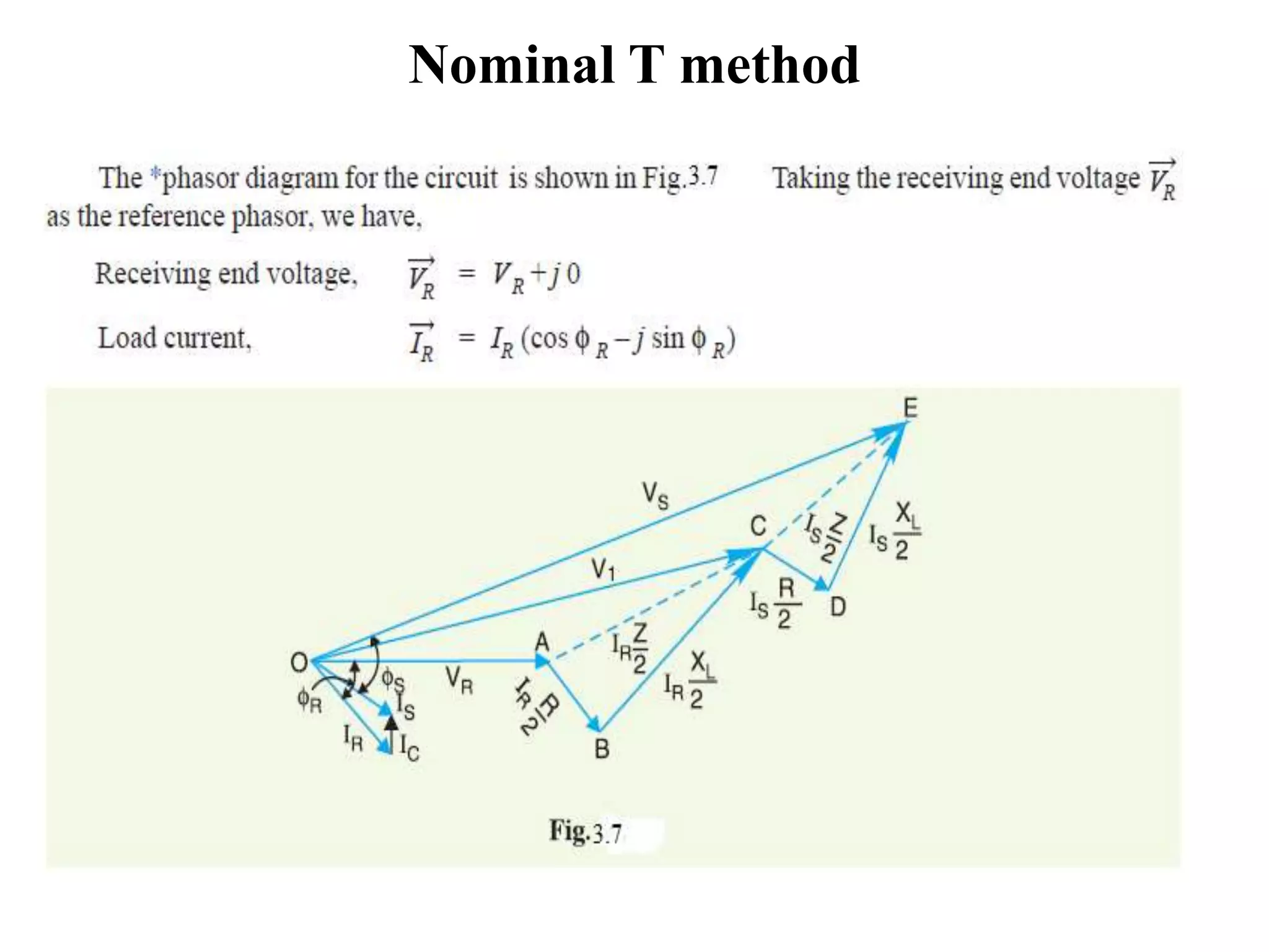
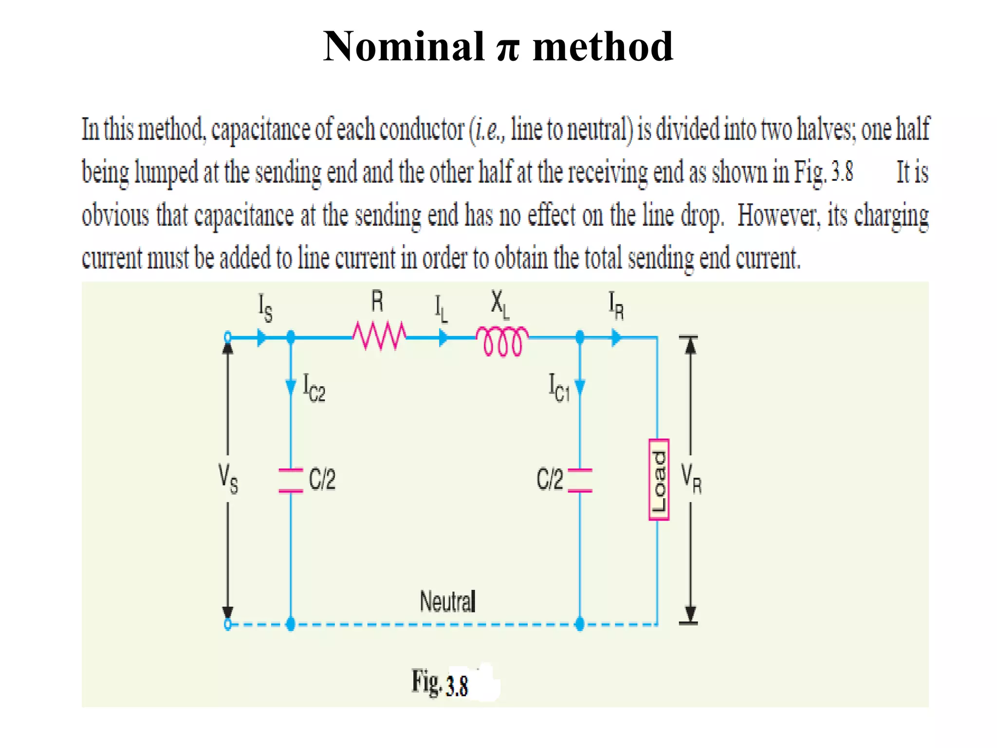
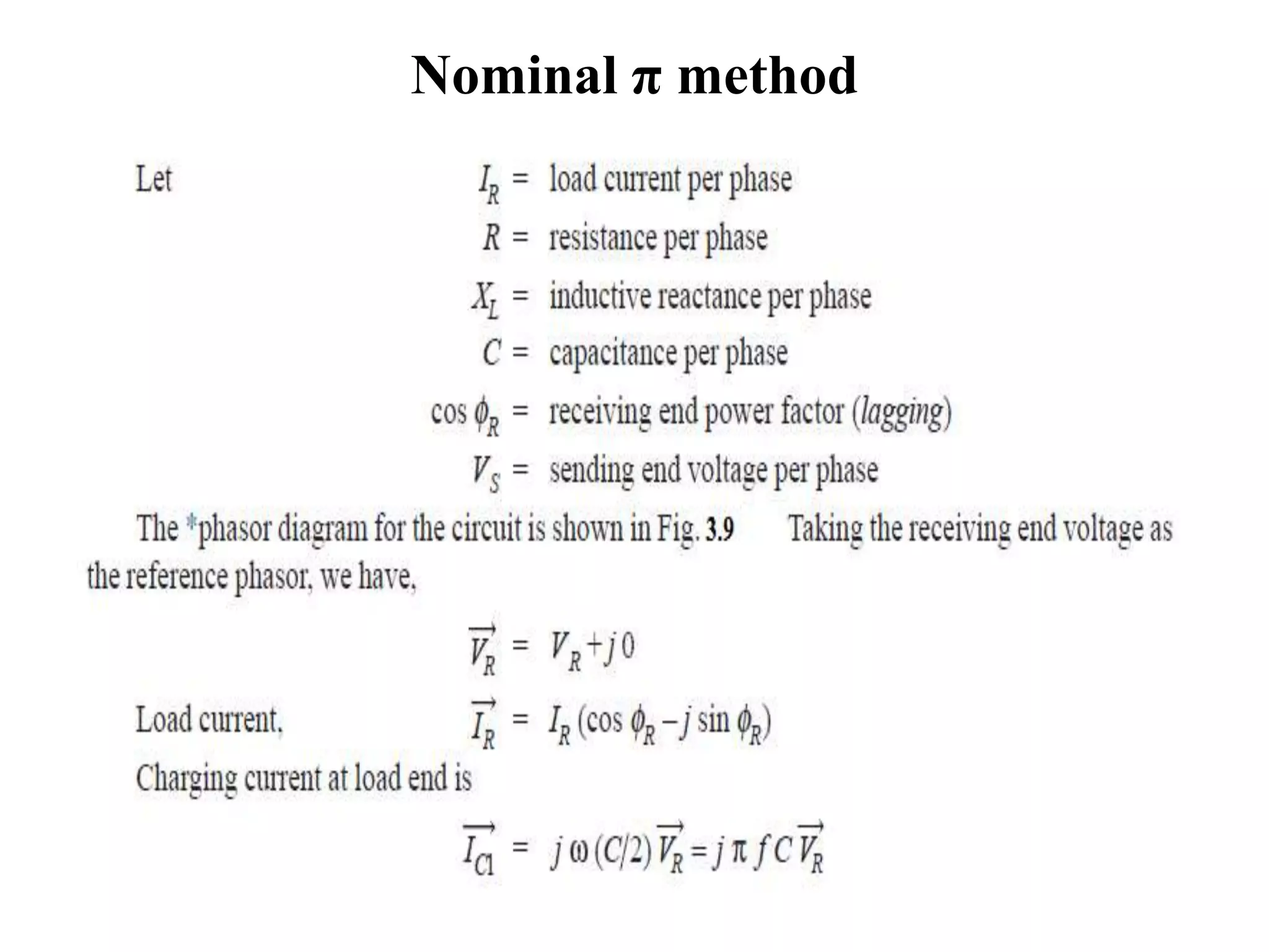
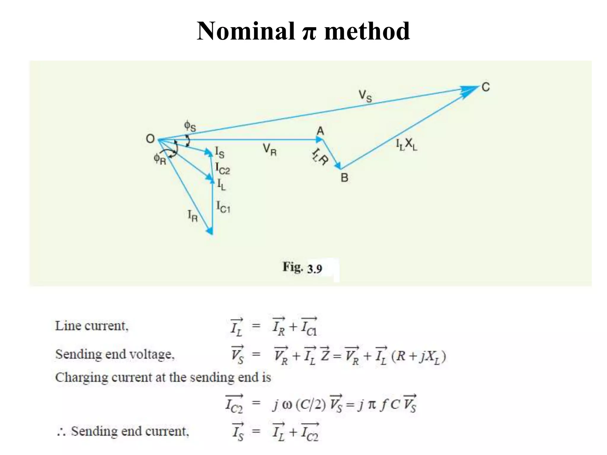
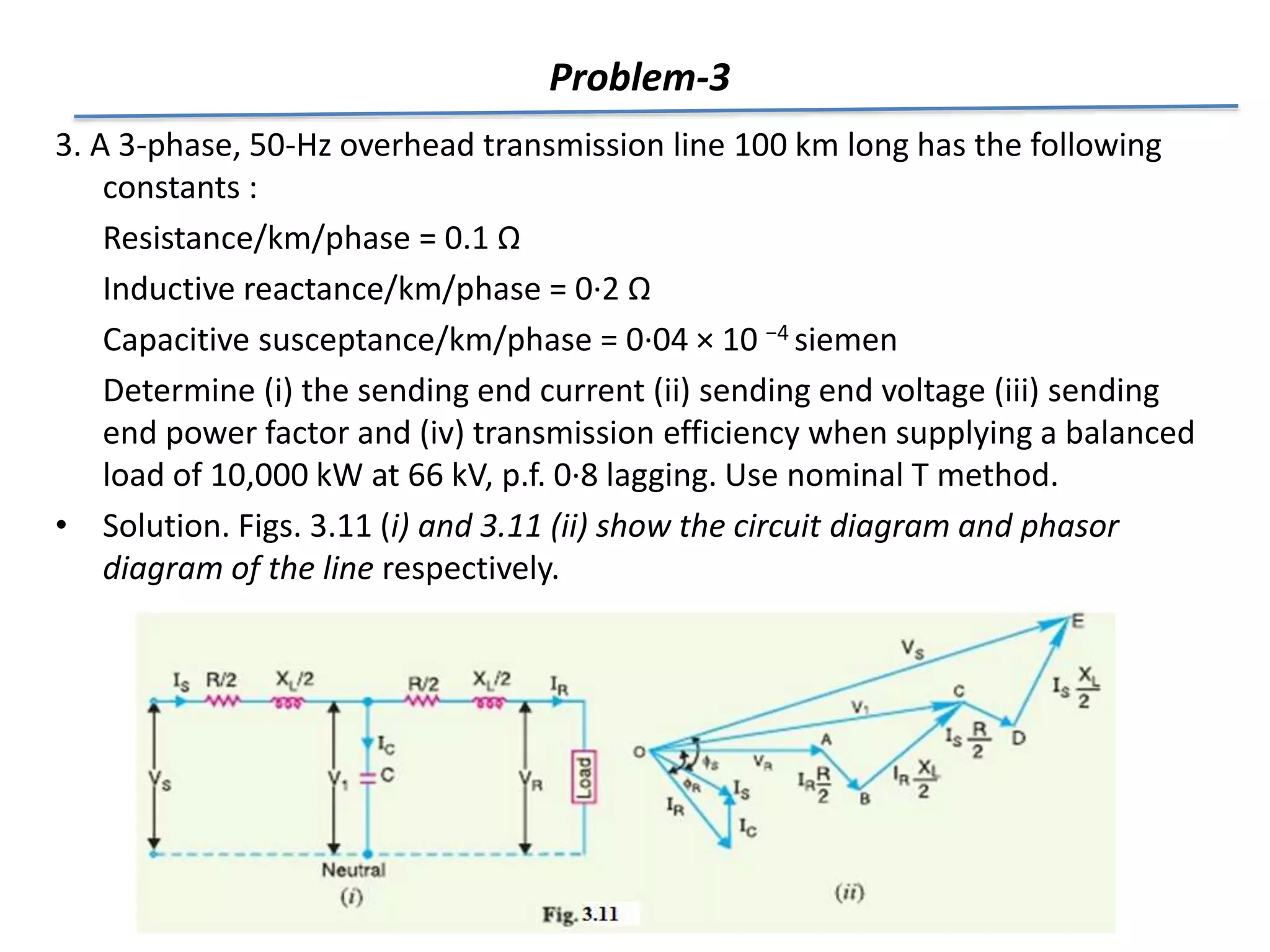
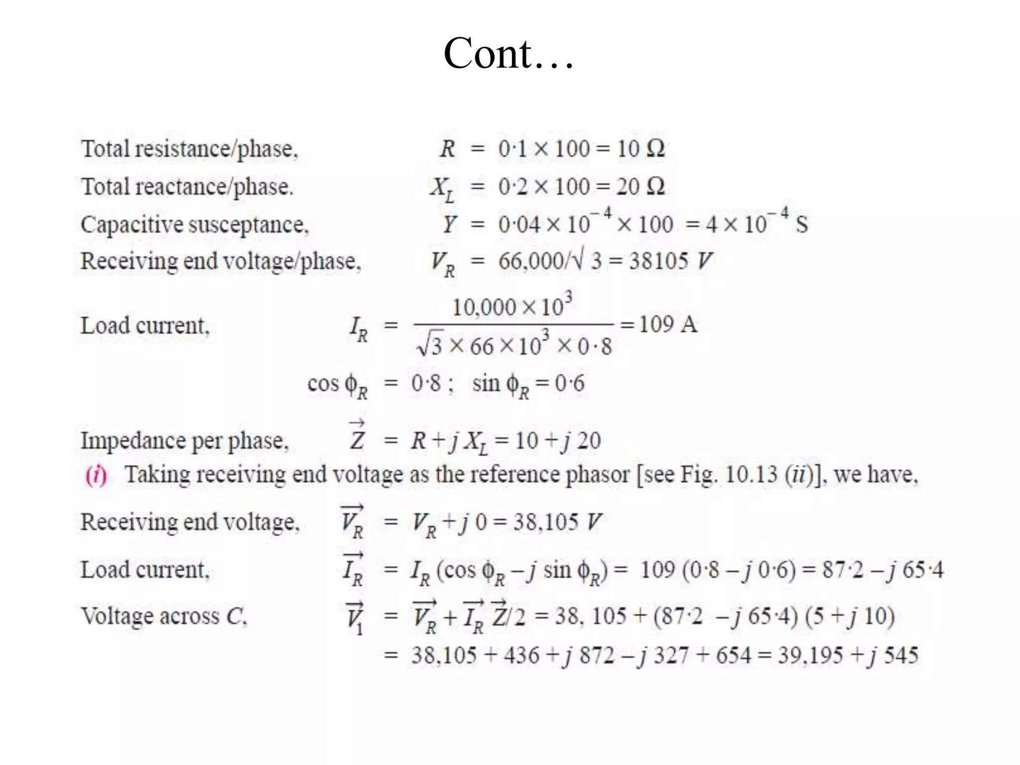
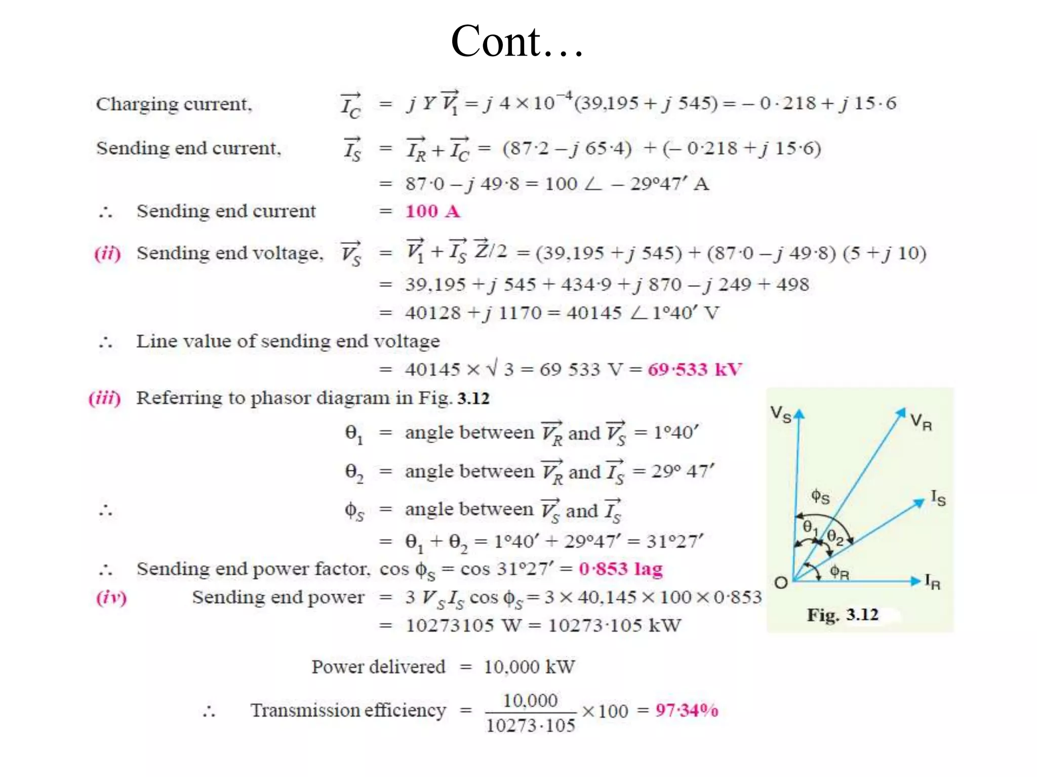
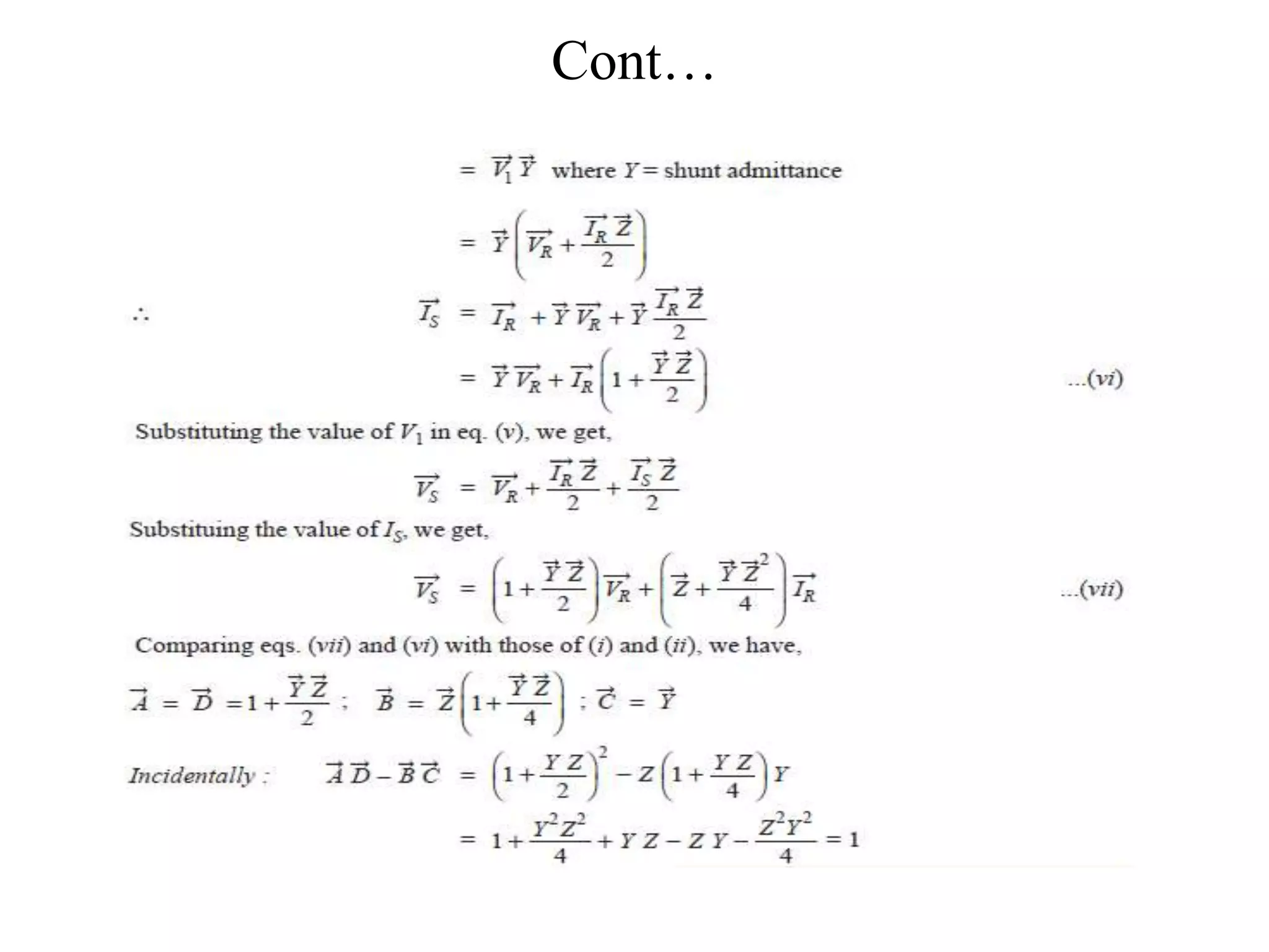
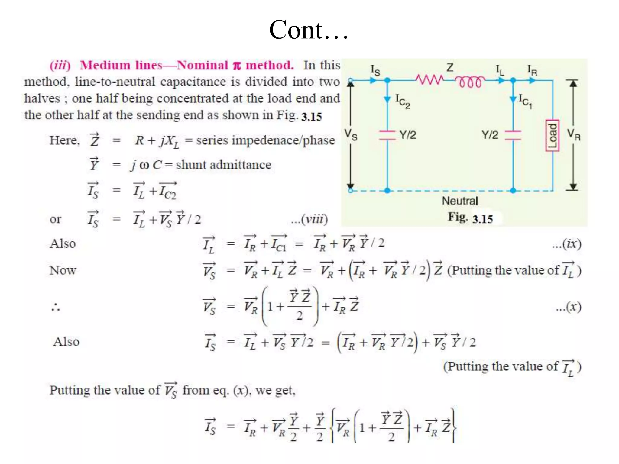
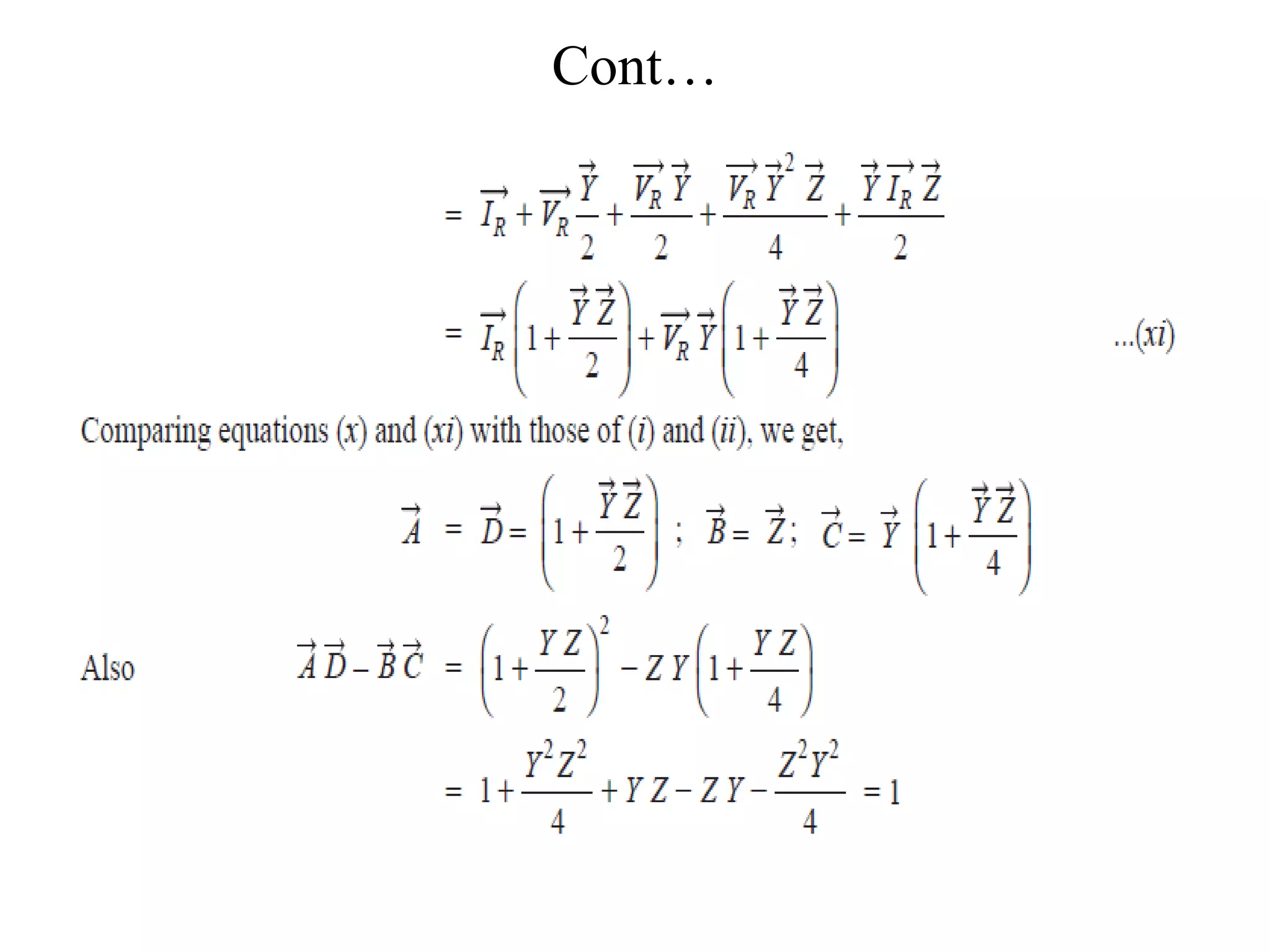
- Medium transmission lines consider capacitance effects by lumping the distributed capacitance at points along the line. Methods like end condenser, nominal T, and nominal pi are commonly used for calculations.
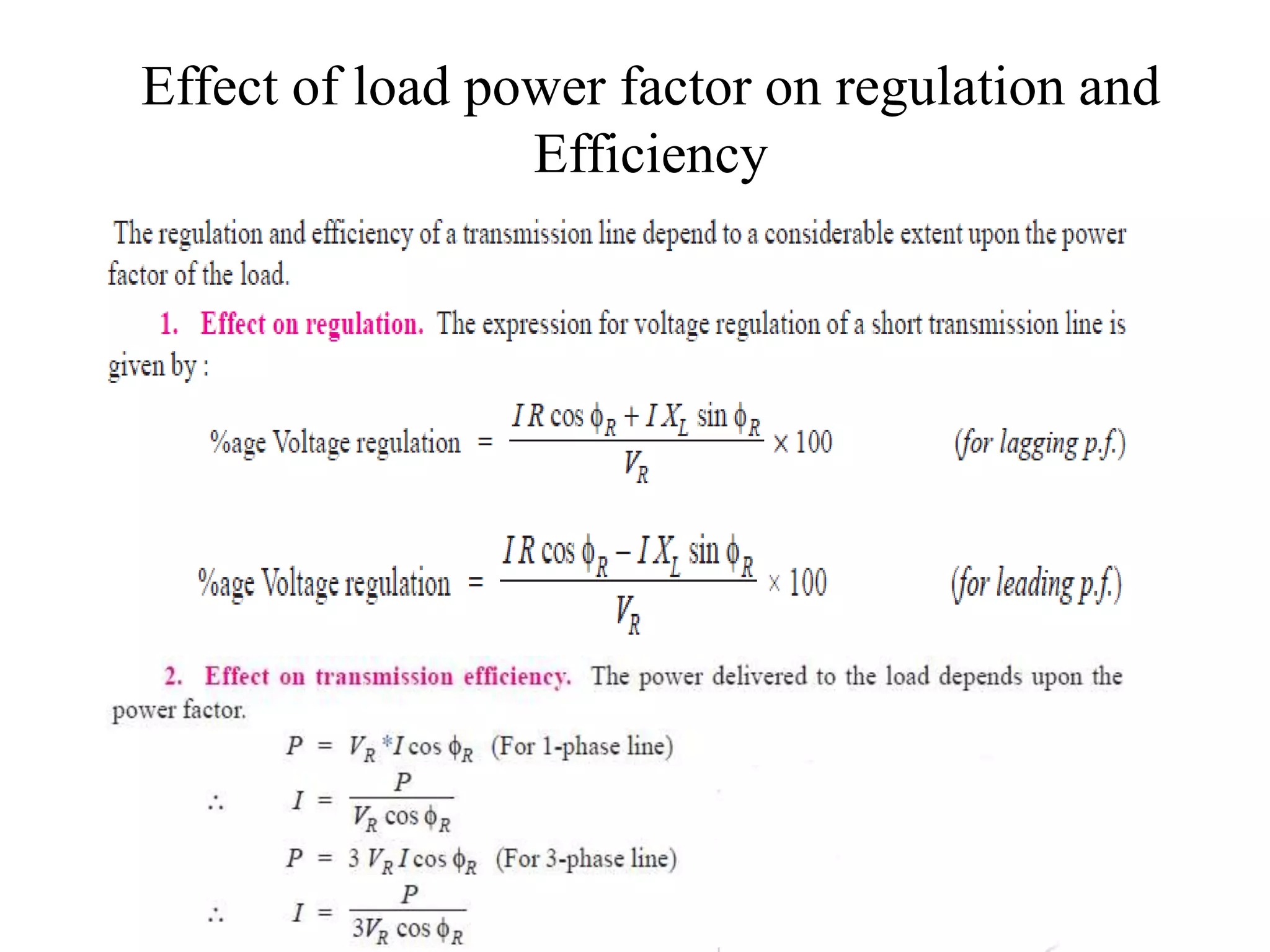
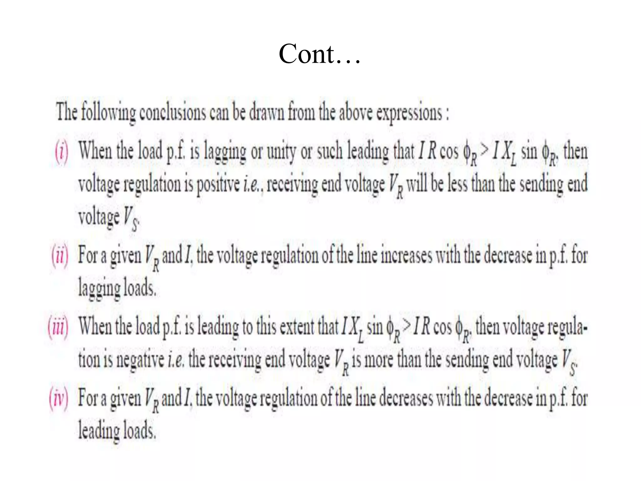
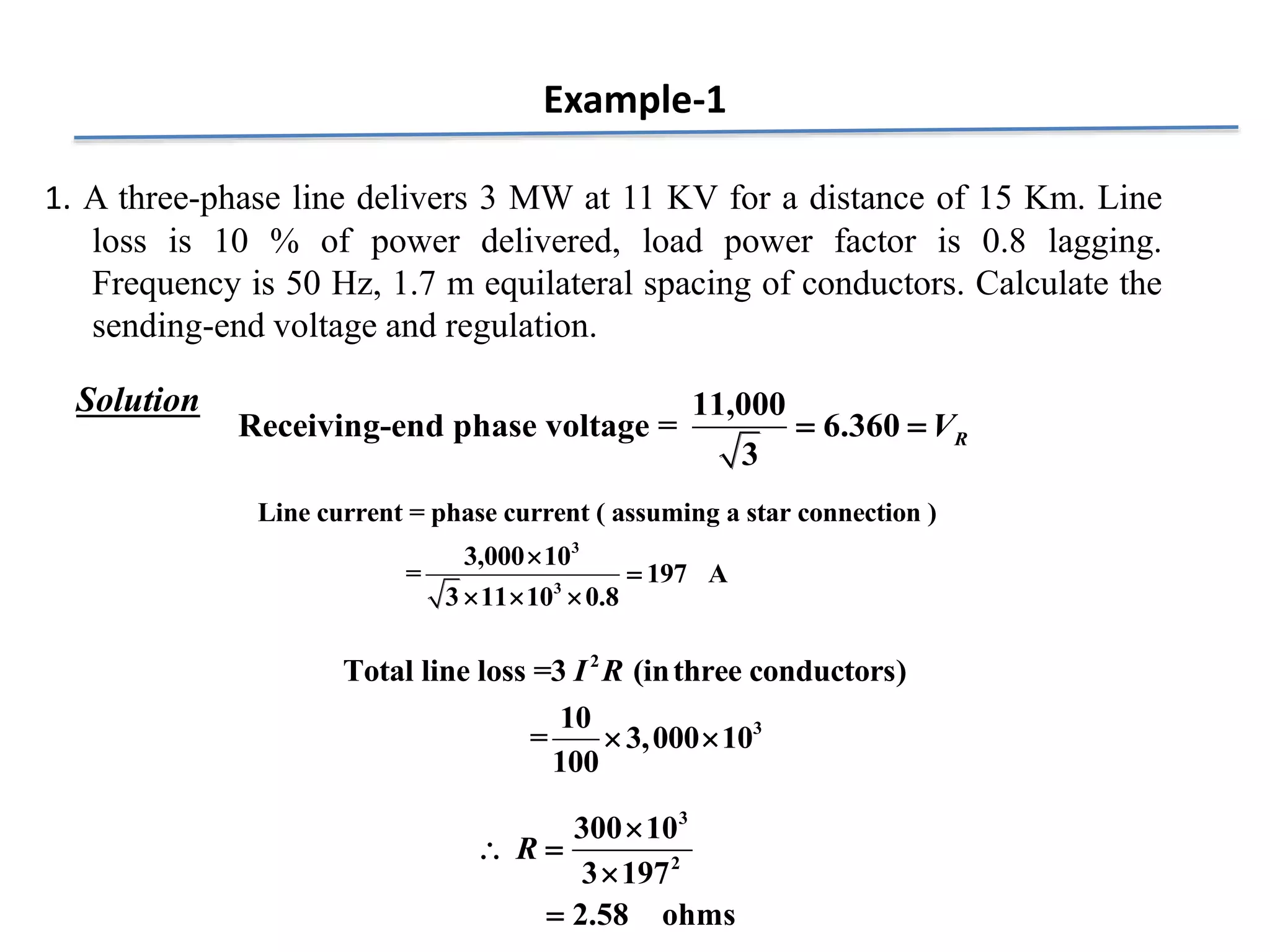
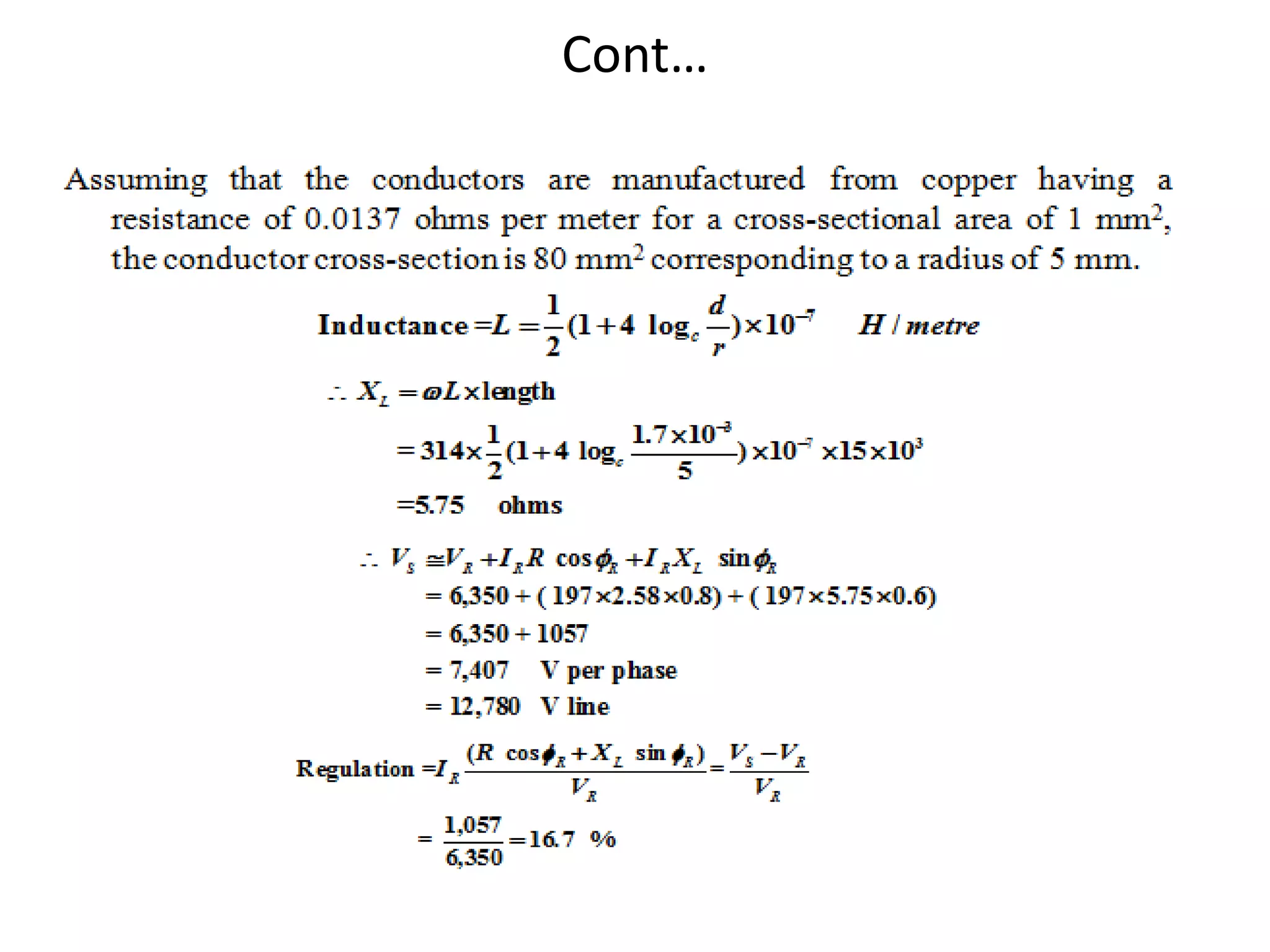
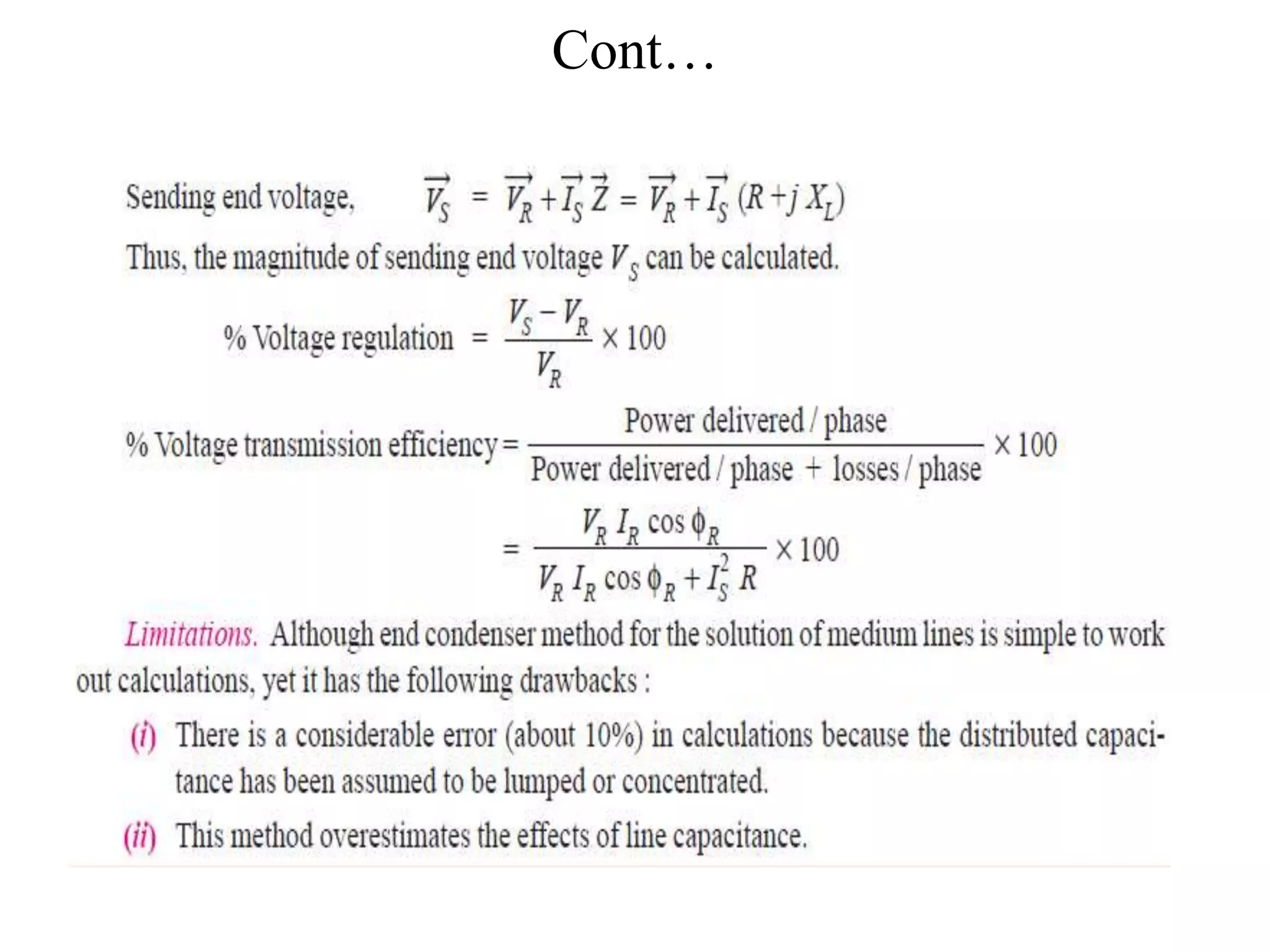
- Examples are provided to demonstrate calculations for voltage regulation,