The document outlines key concepts related to inventory management. It begins with an outline of topics to be covered, including the importance of inventory, types of inventory, and inventory models. The production order quantity model is described, which is used when inventory builds up over time after an order. ABC analysis, cycle counting, and probabilistic inventory models are also mentioned. The document provides examples of calculating optimal order quantities under different models, including economic order quantity, quantity discounts, safety stock, and periodic review systems.

1. 12 - 1
Chapter 12 : Inventory Management

2. 12 - 2
Outline
 The Importance of Inventory
 Functions of Inventory
 Types of Inventory

3. 12 - 3
Outline – Continued
 Managing Inventory
 ABC Analysis
 Record Accuracy
 Cycle Counting
 Control of Service Inventories
 Inventory Models
 Independent vs. Dependent Demand
 Holding, Ordering, and Setup Costs

4. 12 - 4
Outline – Continued
 Inventory Models for Independent
Demand
 The Basic Economic Order Quantity
(EOQ) Model
 Minimizing Costs
 Reorder Points
 Production Order Quantity Model
 Quantity Discount Models

5. 12 - 5
Outline – Continued
 Probabilistic Models and Safety
Stock
 Other Probabilistic Models
 Single-Period Model
 Fixed-Period (P) Systems

6. 12 - 6
Production Order Quantity Model
 Used when inventory builds up
over a period of time after an
order is placed
 Used when units are produced
and sold simultaneously

7. 12 - 7
Production Order Quantity Model
Inventory
level
Time
Demand part of cycle
with no production
Part of inventory cycle during
which production (and usage)
is taking place
t
Maximum
inventory
Figure 12.6

8. 12 - 8
Production Order Quantity Model
Q = Number of pieces per order p = Daily production rate
H = Holding cost per unit per year d = Daily demand/usage rate
t = Length of the production run in days
= (Average inventory level) x
Annual inventory
holding cost
Holding cost
per unit per year
= (Maximum inventory level)/2
Annual inventory
level
= –
Maximum
inventory level
Total produced during
the production run
Total used during
the production run
= pt – dt

9. 12 - 9
Production Order Quantity Model
Q = Number of pieces per order p = Daily production rate
H = Holding cost per unit per year d = Daily demand/usage rate
t = Length of the production run in days
= –
Maximum
inventory level
Total produced during
the production run
Total used during
the production run
= pt – dt
However, Q = total produced = pt ; thus t = Q/p
Maximum
inventory level = p – d = Q 1 –
Q
p
Q
p
d
p
Holding cost = (H) = 1 – H
d
p
Q
2
Maximum inventory level
2

10. 12 - 10
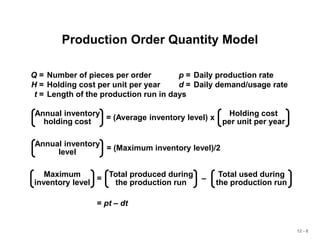
Production Order Quantity Model
Q = Number of pieces per order p = Daily production rate
H = Holding cost per unit per year d = Daily demand/usage rate
D = Annual demand
Q2 =
2DS
H[1 - (d/p)]
Q* =
2DS
H[1 - (d/p)]
p
Setup cost = (D/Q)S
Holding cost = HQ[1 - (d/p)]
1
2
(D/Q)S = HQ[1 - (d/p)]
1
2

11. 12 - 11
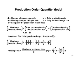
Production Order Quantity Example
D = 1,000 units p = 8 units per day
S = $10 d = 4 units per day
H = $0.50 per unit per year
Q* =
2DS
H[1 - (d/p)]
= 282.8 or 283 hubcaps
Q* = = 80,000
2(1,000)(10)
0.50[1 - (4/8)]

12. 12 - 12
Production Order Quantity Model
When annual data are used the equation becomes
Q* =
2DS
annual demand rate
annual production rate
H 1 –
Note:
d = 4 = =
D
Number of days the plant is in operation
1,000
250

13. 12 - 13
Quantity Discount Models
 Reduced prices are often available when
larger quantities are purchased
 Trade-off is between reduced product cost
and increased holding cost
Total cost = Setup cost + Holding cost + Product cost
TC = S + H + PD
D
Q
Q
2

14. 12 - 14
Quantity Discount Models
Discount
Number Discount Quantity Discount (%)
Discount
Price (P)
1 0 to 999 no discount $5.00
2 1,000 to 1,999 4 $4.80
3 2,000 and over 5 $4.75
Table 12.2
A typical quantity discount schedule

15. 12 - 15
Quantity Discount Models
1. For each discount, calculate Q*
2. If Q* for a discount doesn’t qualify,
choose the smallest possible order size
to get the discount
3. Compute the total cost for each Q* or
adjusted value from Step 2
4. Select the Q* that gives the lowest total
cost
Steps in analyzing a quantity discount

16. 12 - 16
Quantity Discount Models
1,000 2,000
Total
cost
$
0
Order quantity
Q* for discount 2 is below the allowable range at point a
and must be adjusted upward to 1,000 units at point b
a
b
1st price
break
2nd price
break
Total cost
curve for
discount 1
Total cost curve for discount 2
Total cost curve for discount 3
Figure 12.7

17. 12 - 17
Quantity Discount Example
Calculate Q* for every discount Q* =
2DS
IP
Q1* = = 700 cars/order
2(5,000)(49)
(.2)(5.00)
Q2* = = 714 cars/order
2(5,000)(49)
(.2)(4.80)
Q3* = = 718 cars/order
2(5,000)(49)
(.2)(4.75)

18. 12 - 18
Quantity Discount Example
Calculate Q* for every discount Q* =
2DS
IP
Q1* = = 700 cars/order
2(5,000)(49)
(.2)(5.00)
Q2* = = 714 cars/order
2(5,000)(49)
(.2)(4.80)
Q3* = = 718 cars/order
2(5,000)(49)
(.2)(4.75)
1,000 — adjusted
2,000 — adjusted

19. 12 - 19
Quantity Discount Example
Discount
Number
Unit
Price
Order
Quantity
Annual
Product
Cost
Annual
Ordering
Cost
Annual
Holding
Cost Total
1 $5.00 700 $25,000 $350 $350 $25,700
2 $4.80 1,000 $24,000 $245 $480 $24,725
3 $4.75 2,000 $23.750 $122.50 $950 $24,822.50
Table 12.3
Choose the price and quantity that gives
the lowest total cost
Buy 1,000 units at $4.80 per unit

20. 12 - 20
Probabilistic Models and Safety Stock
 Used when demand is not constant
or certain
 Use safety stock to achieve a desired
service level and avoid stockouts
ROP = d x L + ss
Annual stockout costs = the sum of the units short
x the probability x the stockout cost/unit
x the number of orders per year

21. 12 - 21
Safety Stock Example
Number of Units Probability
30 .2
40 .2
ROP  50 .3
60 .2
70 .1
1.0
ROP = 50 units Stockout cost = $40 per frame
Orders per year = 6 Carrying cost = $5 per frame per year

22. 12 - 22
Safety Stock Example
ROP = 50 units Stockout cost = $40 per frame
Orders per year = 6 Carrying cost = $5 per frame per year
Safety
Stock
Additional
Holding Cost Stockout Cost
Total
Cost
20 (20)($5) = $100 $0 $100
10 (10)($5) = $ 50 (10)(.1)($40)(6) = $240 $290
0 $ 0 (10)(.2)($40)(6) + (20)(.1)($40)(6) = $960 $960
A safety stock of 20 frames gives the lowest total cost
ROP = 50 + 20 = 70 frames

23. 12 - 23
Safety stock 16.5 units
ROP 
Place
order
Probabilistic Demand
Inventory
level
Time
0
Minimum demand during lead time
Maximum demand during lead time
Mean demand during lead time
Normal distribution probability of
demand during lead time
Expected demand during lead time (350 kits)
ROP = 350 + safety stock of 16.5 = 366.5
Receive
order
Lead
time
Figure 12.8

24. 12 - 24
Probabilistic Demand
Use prescribed service levels to set safety
stock when the cost of stockouts cannot be
determined
ROP = demand during lead time + ZsdLT
where Z = number of standard deviations
sdLT = standard deviation of demand
during lead time

25. 12 - 25
Probabilistic Demand
Safety
stock
Probability of
no stockout
95% of the time
Mean
demand
350
ROP = ? kits Quantity
Number of
standard deviations
0 z
Risk of a stockout
(5% of area of
normal curve)

26. 12 - 26
Probabilistic Example
Average demand = m = 350 kits
Standard deviation of demand during lead time = sdLT = 10 kits
5% stockout policy (service level = 95%)
Using Appendix I, for an area under the curve
of 95%, the Z = 1.65
Safety stock = ZsdLT = 1.65(10) = 16.5 kits
Reorder point = expected demand during lead time
+ safety stock
= 350 kits + 16.5 kits of safety stock
= 366.5 or 367 kits

27. 12 - 27
Other Probabilistic Models
1. When demand is variable and lead
time is constant
2. When lead time is variable and
demand is constant
3. When both demand and lead time
are variable
When data on demand during lead time is
not available, there are other models
available

28. 12 - 28
Other Probabilistic Models
Demand is variable and lead time is constant
ROP = (average daily demand
x lead time in days) + ZsdLT
where sd = standard deviation of demand per day
sdLT = sd lead time

29. 12 - 29
Probabilistic Example
Average daily demand (normally distributed) = 15
Standard deviation = 5
Lead time is constant at 2 days
90% service level desired
Z for 90% = 1.28
From Appendix I
ROP = (15 units x 2 days) + ZsdLT
= 30 + 1.28(5)( 2)
= 30 + 9.02 = 39.02 ≈ 39
Safety stock is about 9 iPods

30. 12 - 30
Other Probabilistic Models
Lead time is variable and demand is constant
ROP = (daily demand x average lead
time in days)
= Z x (daily demand) x sLT
where sLT = standard deviation of lead time in days

31. 12 - 31
Probabilistic Example
Daily demand (constant) = 10
Average lead time = 6 days
Standard deviation of lead time = sLT = 3
98% service level desired
Z for 98% = 2.055
From Appendix I
ROP = (10 units x 6 days) + 2.055(10 units)(3)
= 60 + 61.65 = 121.65
Reorder point is about 122 cameras

32. 12 - 32
Other Probabilistic Models
Both demand and lead time are variable
ROP = (average daily demand
x average lead time) + ZsdLT
where sd = standard deviation of demand per day
sLT = standard deviation of lead time in days
sdLT = (average lead time x sd
2)
+ (average daily demand)2 x sLT
2

33. 12 - 33
Probabilistic Example
Average daily demand (normally distributed) = 150
Standard deviation = sd = 16
Average lead time 5 days (normally distributed)
Standard deviation = sLT = 1 day
95% service level desired Z for 95% = 1.65
From Appendix I
ROP = (150 packs x 5 days) + 1.65sdLT
= (150 x 5) + 1.65 (5 days x 162) + (1502 x 12)
= 750 + 1.65(154) = 1,004 packs

34. 12 - 34
Single Period Model
 Only one order is placed for a product
 Units have little or no value at the end of the
sales period
Cs = Cost of shortage = Sales price/unit – Cost/unit
Co = Cost of overage = Cost/unit – Salvage value
Service level =
Cs
Cs + Co

35. 12 - 35
Single Period Example
Average demand = m = 120 papers/day
Standard deviation = s = 15 papers
Cs = cost of shortage = $1.25 - $.70 = $.55
Co = cost of overage = $.70 - $.30 = $.40
Service level =
Cs
Cs + Co
.55
.55 + .40
.55
.95
=
= = .578
Service
level
57.8%
Optimal stocking level
m = 120

36. 12 - 36
Single Period Example
From Appendix I, for the area .578, Z  .20
The optimal stocking level
= 120 copies + (.20)(s)
= 120 + (.20)(15) = 120 + 3 = 123 papers
The stockout risk = 1 – service level
= 1 – .578 = .422 = 42.2%

37. 12 - 37
Fixed-Period (P) Systems
 Orders placed at the end of a fixed period
 Inventory counted only at end of period
 Order brings inventory up to target level
 Only relevant costs are ordering and holding
 Lead times are known and constant
 Items are independent from one another

38. 12 - 38
Fixed-Period (P) Systems
On-hand
inventory
Time
Q1
Q2
Target quantity (T)
P
Q3
Q4
P
P
Figure 12.9

39. 12 - 39
Fixed-Period (P) Example
Order amount (Q) = Target (T) - On-
hand inventory - Earlier orders not yet
received + Back orders
Q = 50 - 0 - 0 + 3 = 53 jackets
3 jackets are back ordered No jackets are in stock
It is time to place an order Target value = 50

40. 12 - 40
Fixed-Period Systems
 Inventory is only counted at each
review period
 May be scheduled at convenient times
 Appropriate in routine situations
 May result in stockouts between
periods
 May require increased safety stock