Downloaded 310 times


![21
ModelingModeling
Mathematical representation of the physical problem
– Some problems are exact (e.g., laminar pipe flow)
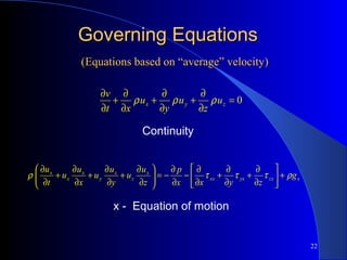
– Exact solutions only exist for some simple cases. In
these cases nonlinear terms can be dropped from the N-
S equations which allow analytical solution.
– Most cases require models for flow behavior [e.g.,
Reynolds Averaged Navier Stokes equations (RANS)
or Large Eddy Simulation (LES) for turbulent flow]
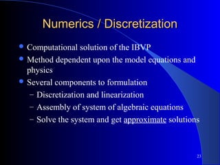
Initial —Boundary Value Problem (IBVP), include:
governing Partial Differential Equations (PDEs), Initial
Conditions (ICs) and Boundary Conditions (BCs)](https://image.slidesharecdn.com/cfdpresentation-170330093525/85/Introduction-to-Computational-Fluid-Dynamics-CFD-21-320.jpg)
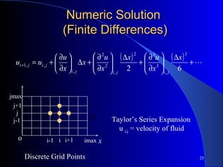
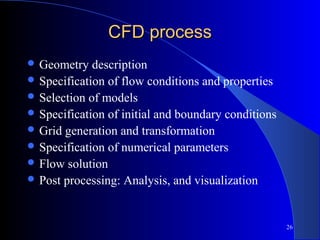
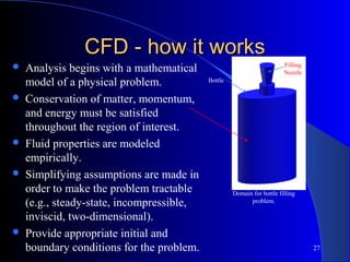
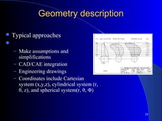
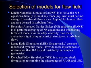
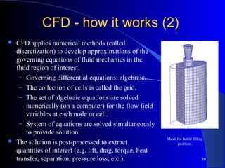
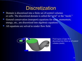


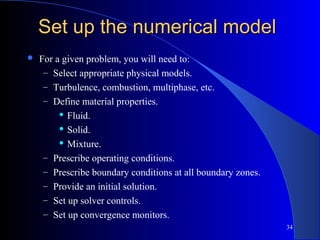


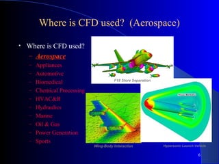
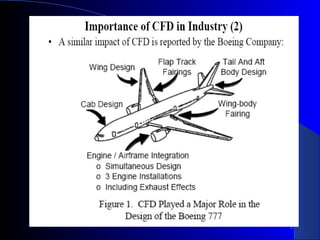
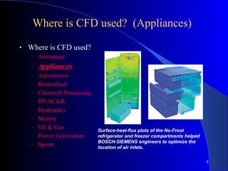
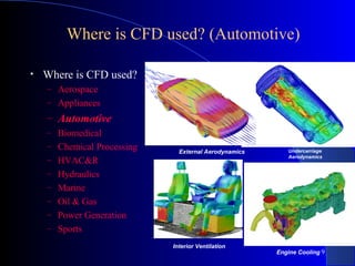
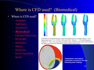
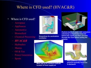
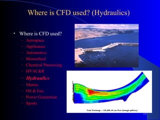
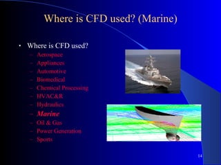
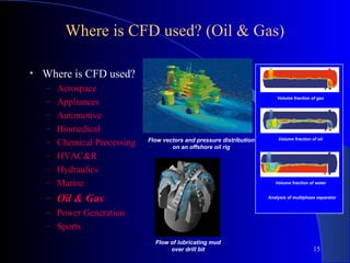
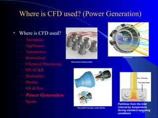
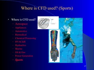
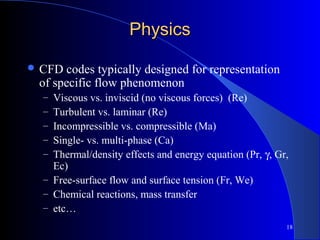
This document provides an overview of computational fluid dynamics (CFD). It defines CFD as using computer simulations to predict fluid flow phenomena by modeling continuous fluids with partial differential equations. The document outlines where CFD is used in various industries like aerospace, automotive, biomedical, and more. It also discusses the physics, modeling, numerics, and overall CFD process involved in simulations. Examples are given of mesh generation and CFD being used to analyze problems like bottle filling.