CFD

1. Introduction to
Computational Fluid
Dynamics (CFD)
Tao Xing, Shanti Bhushan and Fred Stern
IIHR—Hydroscience & Engineering
C. Maxwell Stanley Hydraulics Laboratory
The University of Iowa
57:020 Mechanics of Fluids and Transport Processes
http://css.engineering.uiowa.edu/~fluids/
Ocrtober 7, 2009

2. 2
Outline
1. What, why and where of CFD?
2. Modeling
3. Numerical methods
4. Types of CFD codes
5. CFD Educational Interface
6. CFD Process
7. Example of CFD Process
8. 57:020 CFD Labs

3. 3
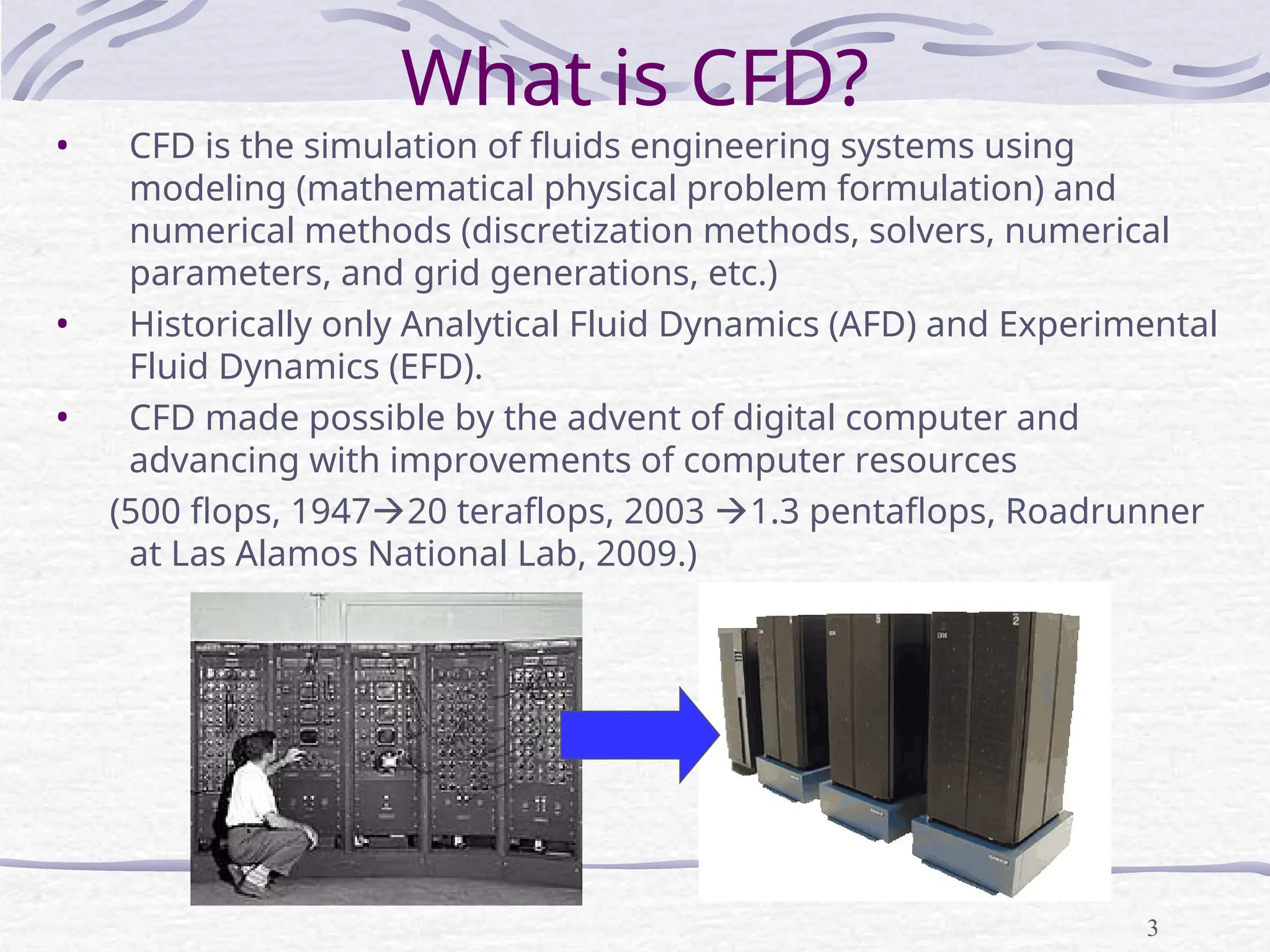
What is CFD?
• CFD is the simulation of fluids engineering systems using
modeling (mathematical physical problem formulation) and
numerical methods (discretization methods, solvers, numerical
parameters, and grid generations, etc.)
• Historically only Analytical Fluid Dynamics (AFD) and Experimental
Fluid Dynamics (EFD).
• CFD made possible by the advent of digital computer and
advancing with improvements of computer resources
(500 flops, 194720 teraflops, 2003 1.3 pentaflops, Roadrunner
at Las Alamos National Lab, 2009.)

4. 4
Why use CFD?
• Analysis and Design
1. Simulation-based design instead of “build & test”
More cost effective and more rapid than EFD
CFD provides high-fidelity database for diagnosing flow
field
2. Simulation of physical fluid phenomena that are
difficult for experiments
Full scale simulations (e.g., ships and airplanes)
Environmental effects (wind, weather, etc.)
Hazards (e.g., explosions, radiation, pollution)
Physics (e.g., planetary boundary layer, stellar
evolution)
• Knowledge and exploration of flow physics

5. 5
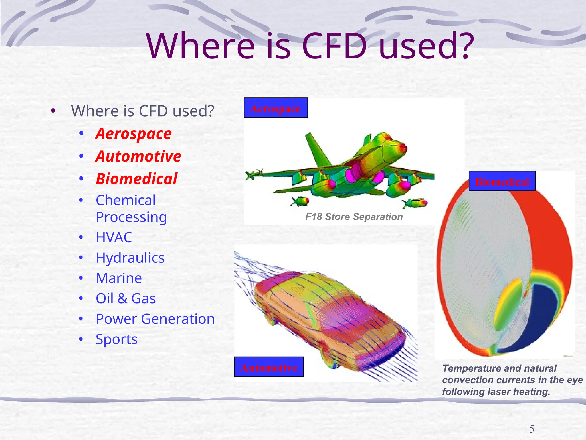
Where is CFD used?
• Where is CFD used?
• Aerospace
• Automotive
• Biomedical
• Chemical
Processing
• HVAC
• Hydraulics
• Marine
• Oil & Gas
• Power Generation
• Sports
F18 Store Separation
Temperature and natural
convection currents in the eye
following laser heating.
Aerospace
Automotive
Biomedical

6. 6
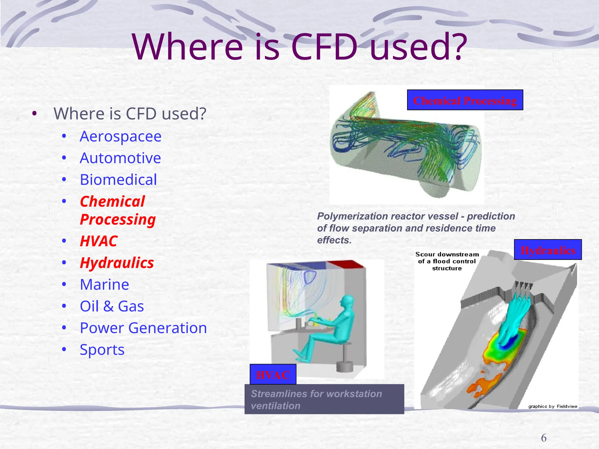
Where is CFD used?
Polymerization reactor vessel - prediction
of flow separation and residence time
effects.
Streamlines for workstation
ventilation
• Where is CFD used?
• Aerospacee
• Automotive
• Biomedical
• Chemical
Processing
• HVAC
• Hydraulics
• Marine
• Oil & Gas
• Power Generation
• Sports
HVAC
Chemical Processing
Hydraulics

7. 7
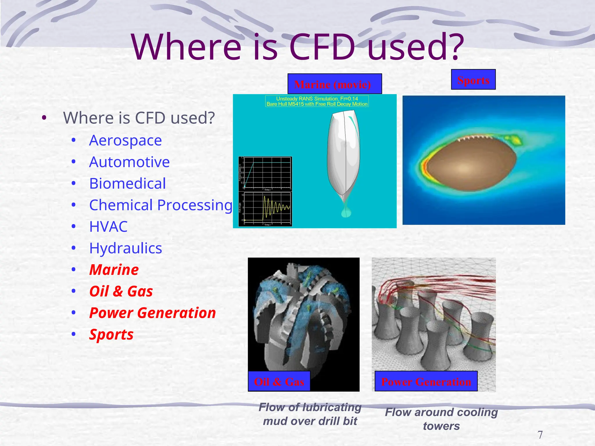
Where is CFD used?
• Where is CFD used?
• Aerospace
• Automotive
• Biomedical
• Chemical Processing
• HVAC
• Hydraulics
• Marine
• Oil & Gas
• Power Generation
• Sports
Flow of lubricating
mud over drill bit
Flow around cooling
towers
Marine (movie)
Oil & Gas
Sports
Power Generation

8. 8
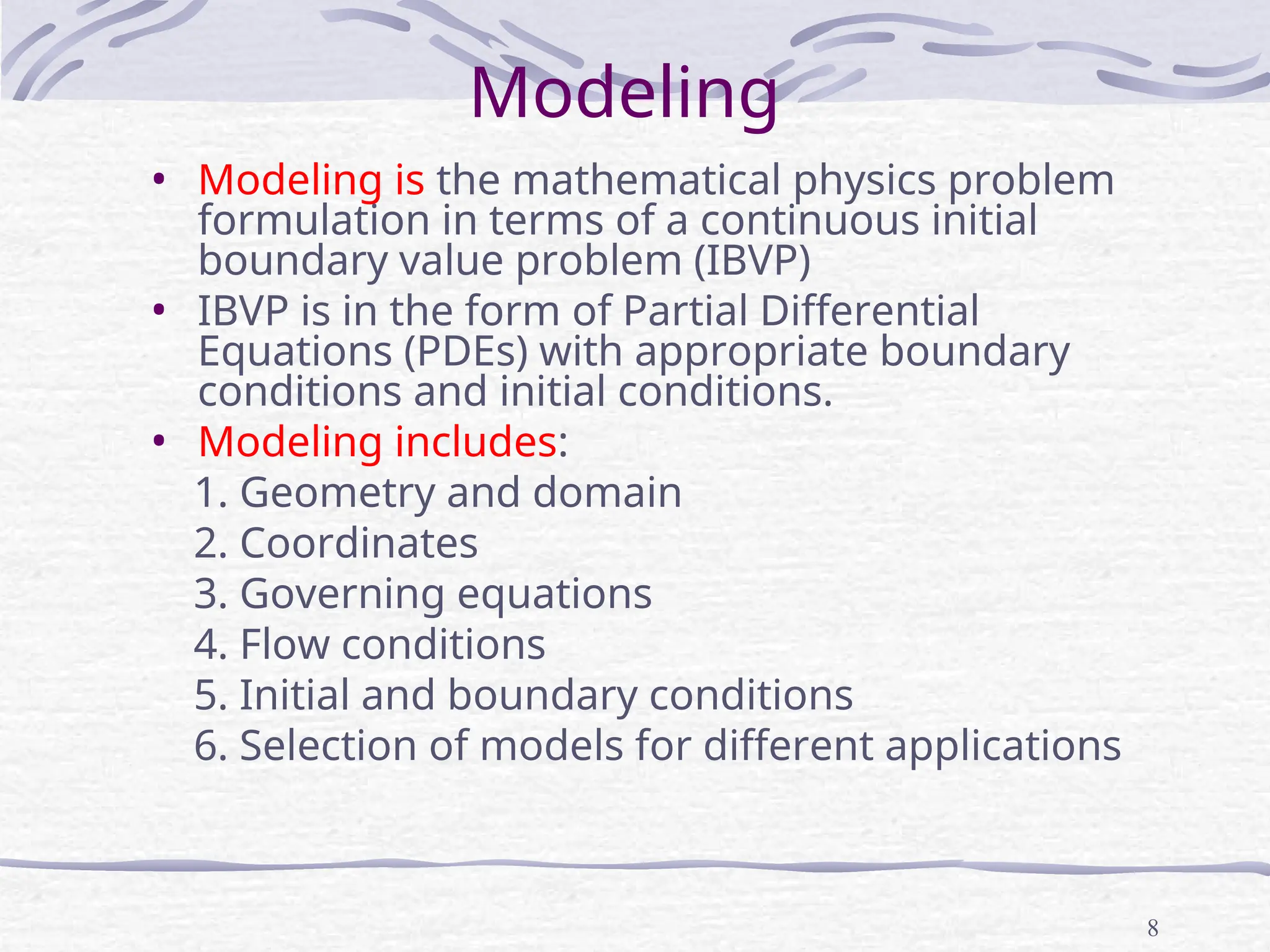
Modeling
• Modeling is the mathematical physics problem
formulation in terms of a continuous initial
boundary value problem (IBVP)
• IBVP is in the form of Partial Differential
Equations (PDEs) with appropriate boundary
conditions and initial conditions.
• Modeling includes:
1. Geometry and domain
2. Coordinates
3. Governing equations
4. Flow conditions
5. Initial and boundary conditions
6. Selection of models for different applications

9. 9
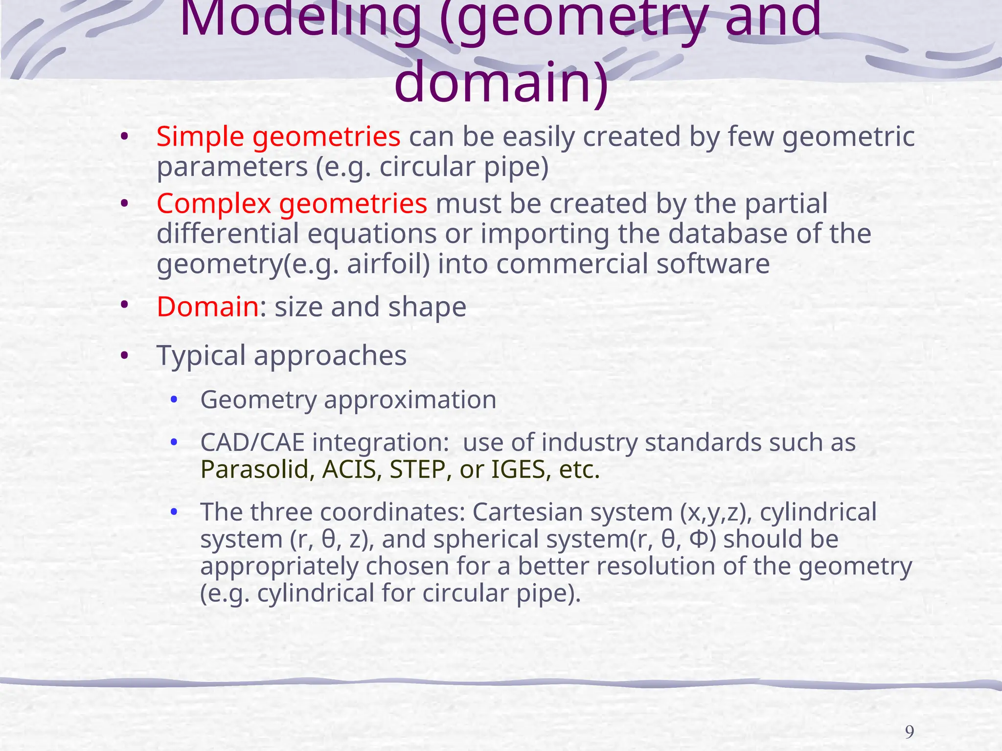
Modeling (geometry and
domain)
• Simple geometries can be easily created by few geometric
parameters (e.g. circular pipe)
• Complex geometries must be created by the partial
differential equations or importing the database of the
geometry(e.g. airfoil) into commercial software
• Domain: size and shape
• Typical approaches
• Geometry approximation
• CAD/CAE integration: use of industry standards such as
Parasolid, ACIS, STEP, or IGES, etc.
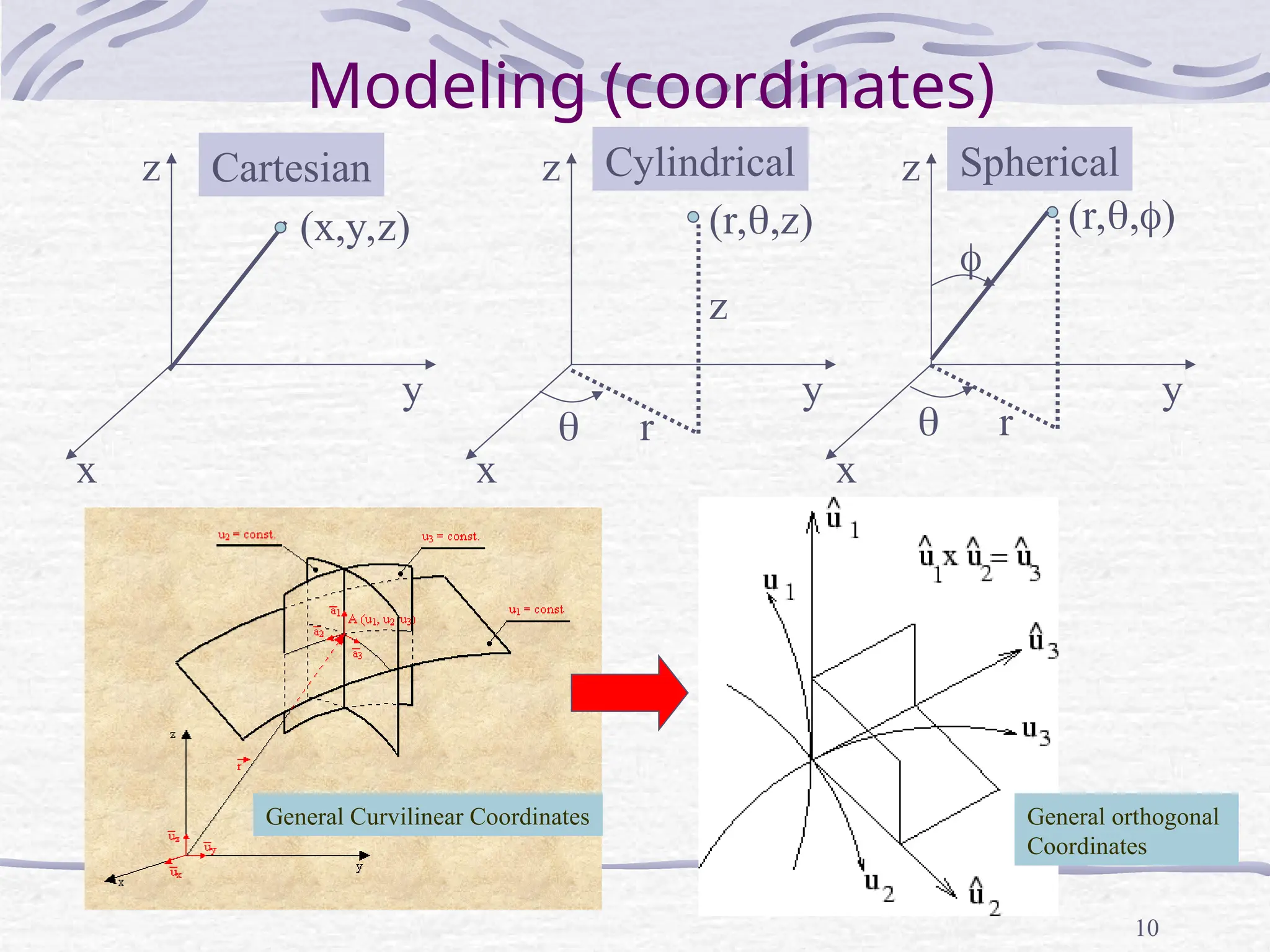
• The three coordinates: Cartesian system (x,y,z), cylindrical
system (r, θ, z), and spherical system(r, θ, Φ) should be
appropriately chosen for a better resolution of the geometry
(e.g. cylindrical for circular pipe).

10. 10
Modeling (coordinates)
x
y
z
x
y
z
x
y
z
(r,,z)
z
r

(r,,)
r


(x,y,z)
Cartesian Cylindrical Spherical
General Curvilinear Coordinates General orthogonal
Coordinates

11. 11
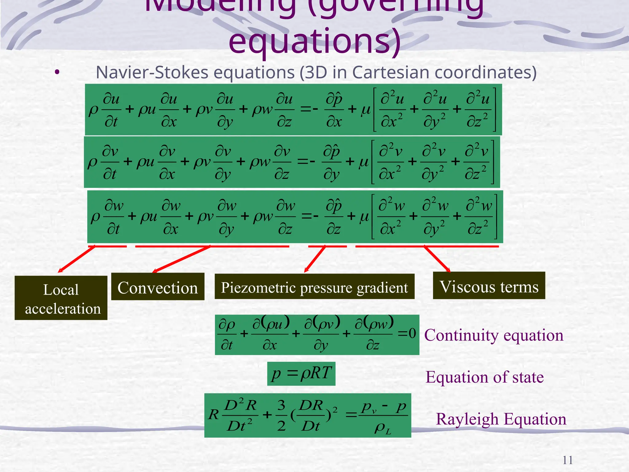
Modeling (governing
equations)
• Navier-Stokes equations (3D in Cartesian coordinates)






























2
2
2
2
2
2
ˆ
z
u
y
u
x
u
x
p
z
u
w
y
u
v
x
u
u
t
u



































2
2
2
2
2
2
ˆ
z
v
y
v
x
v
y
p
z
v
w
y
v
v
x
v
u
t
v





      0












z
w
y
v
x
u
t




RT
p 

L
v p
p
Dt
DR
Dt
R
D
R



 2
2
2
)
(
2
3
Convection Piezometric pressure gradient Viscous terms
Local
acceleration
Continuity equation
Equation of state
Rayleigh Equation






























2
2
2
2
2
2
ˆ
z
w
y
w
x
w
z
p
z
w
w
y
w
v
x
w
u
t
w






12. 12
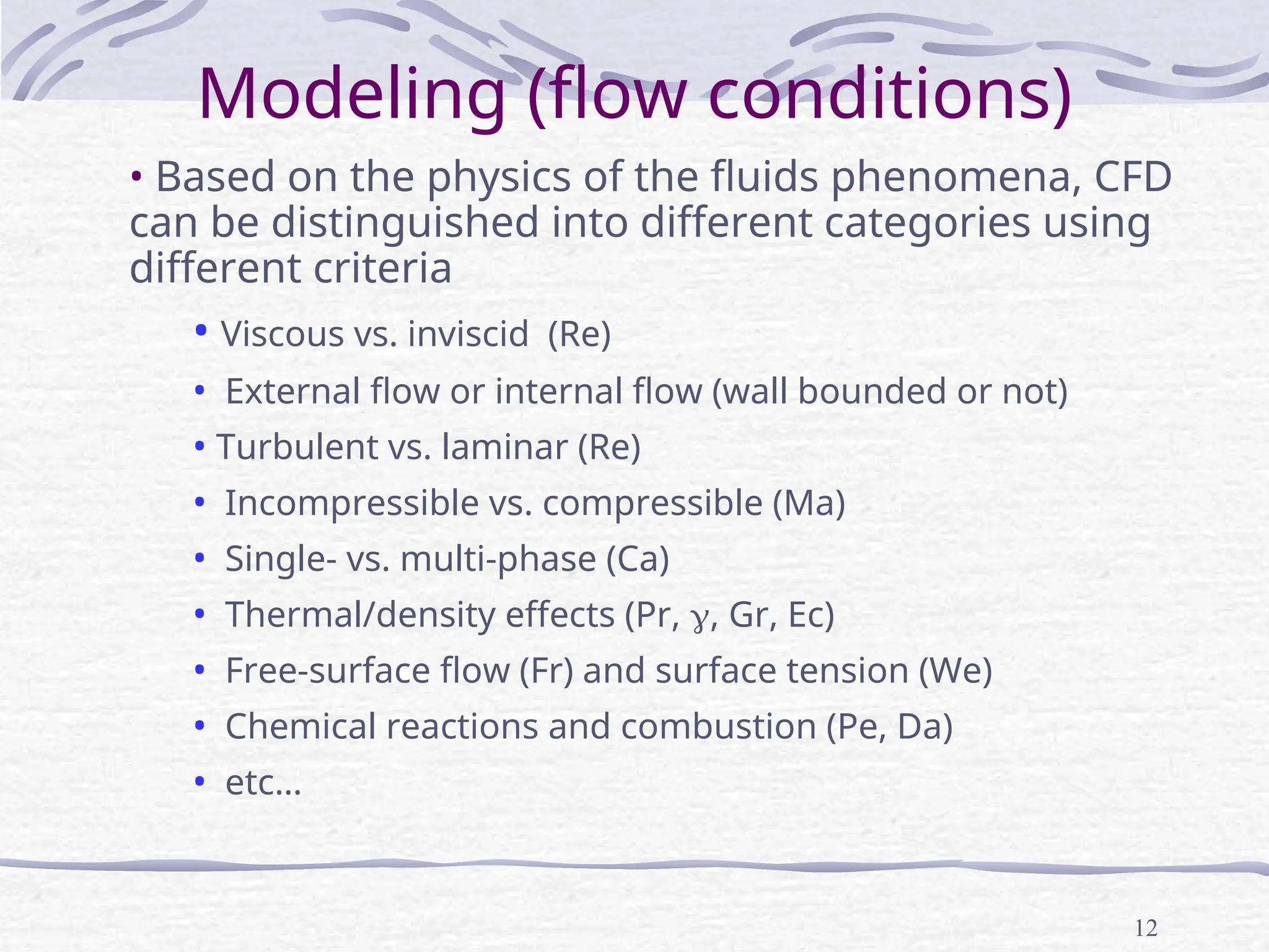
Modeling (flow conditions)
• Based on the physics of the fluids phenomena, CFD
can be distinguished into different categories using
different criteria
• Viscous vs. inviscid (Re)
• External flow or internal flow (wall bounded or not)
• Turbulent vs. laminar (Re)
• Incompressible vs. compressible (Ma)
• Single- vs. multi-phase (Ca)
• Thermal/density effects (Pr, , Gr, Ec)
• Free-surface flow (Fr) and surface tension (We)
• Chemical reactions and combustion (Pe, Da)
• etc…

13. 13
Modeling (initial conditions)
• Initial conditions (ICS, steady/unsteady flows)
• ICs should not affect final results and only
affect convergence path, i.e. number of
iterations (steady) or time steps (unsteady)
need to reach converged solutions.
• More reasonable guess can speed up the
convergence
• For complicated unsteady flow problems,
CFD codes are usually run in the steady
mode for a few iterations for getting a
better initial conditions

14. 14
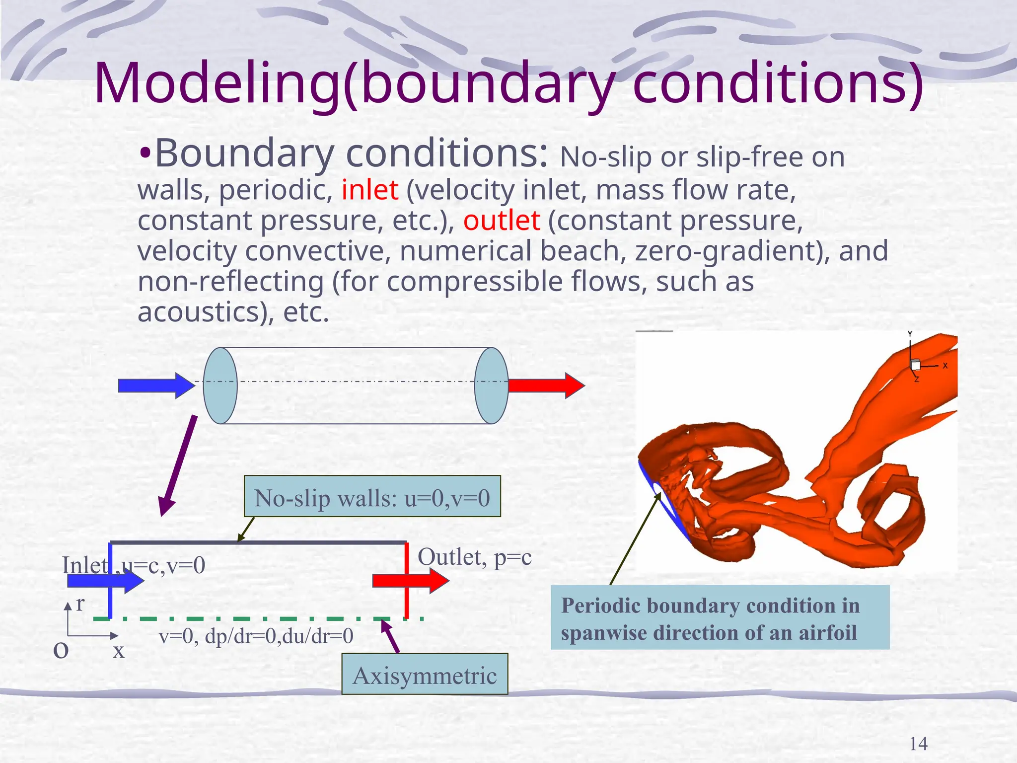
Modeling(boundary conditions)
•Boundary conditions: No-slip or slip-free on
walls, periodic, inlet (velocity inlet, mass flow rate,
constant pressure, etc.), outlet (constant pressure,
velocity convective, numerical beach, zero-gradient), and
non-reflecting (for compressible flows, such as
acoustics), etc.
No-slip walls: u=0,v=0
v=0, dp/dr=0,du/dr=0
Inlet ,u=c,v=0 Outlet, p=c
Periodic boundary condition in
spanwise direction of an airfoil
o
r
x
Axisymmetric

15. 15
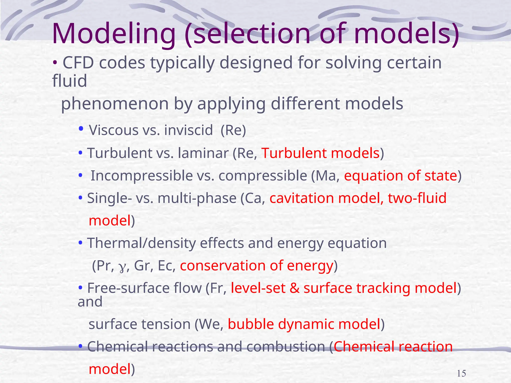
Modeling (selection of models)
• CFD codes typically designed for solving certain
fluid
phenomenon by applying different models
• Viscous vs. inviscid (Re)
• Turbulent vs. laminar (Re, Turbulent models)
• Incompressible vs. compressible (Ma, equation of state)
• Single- vs. multi-phase (Ca, cavitation model, two-fluid
model)
• Thermal/density effects and energy equation
(Pr, , Gr, Ec, conservation of energy)
• Free-surface flow (Fr, level-set & surface tracking model)
and
surface tension (We, bubble dynamic model)
• Chemical reactions and combustion (Chemical reaction
model)

16. 16
Modeling (Turbulence and free surface
models)
• Turbulent models:
• DNS: most accurately solve NS equations, but too expensive
for turbulent flows
• RANS: predict mean flow structures, efficient inside BL but
excessive
diffusion in the separated region.
• LES: accurate in separation region and unaffordable for resolving
BL
• DES: RANS inside BL, LES in separated regions.
• Free-surface models:
• Surface-tracking method: mesh moving to capture free surface,
limited to small and medium wave slopes
• Single/two phase level-set method: mesh fixed and level-set
function used to capture the gas/liquid interface, capable of
studying steep or breaking waves.
• Turbulent flows at high Re usually involve both large and small scale
vortical structures and very thin turbulent boundary layer (BL) near the
wall

17. 17
Examples of modeling (Turbulence and
free surface models)
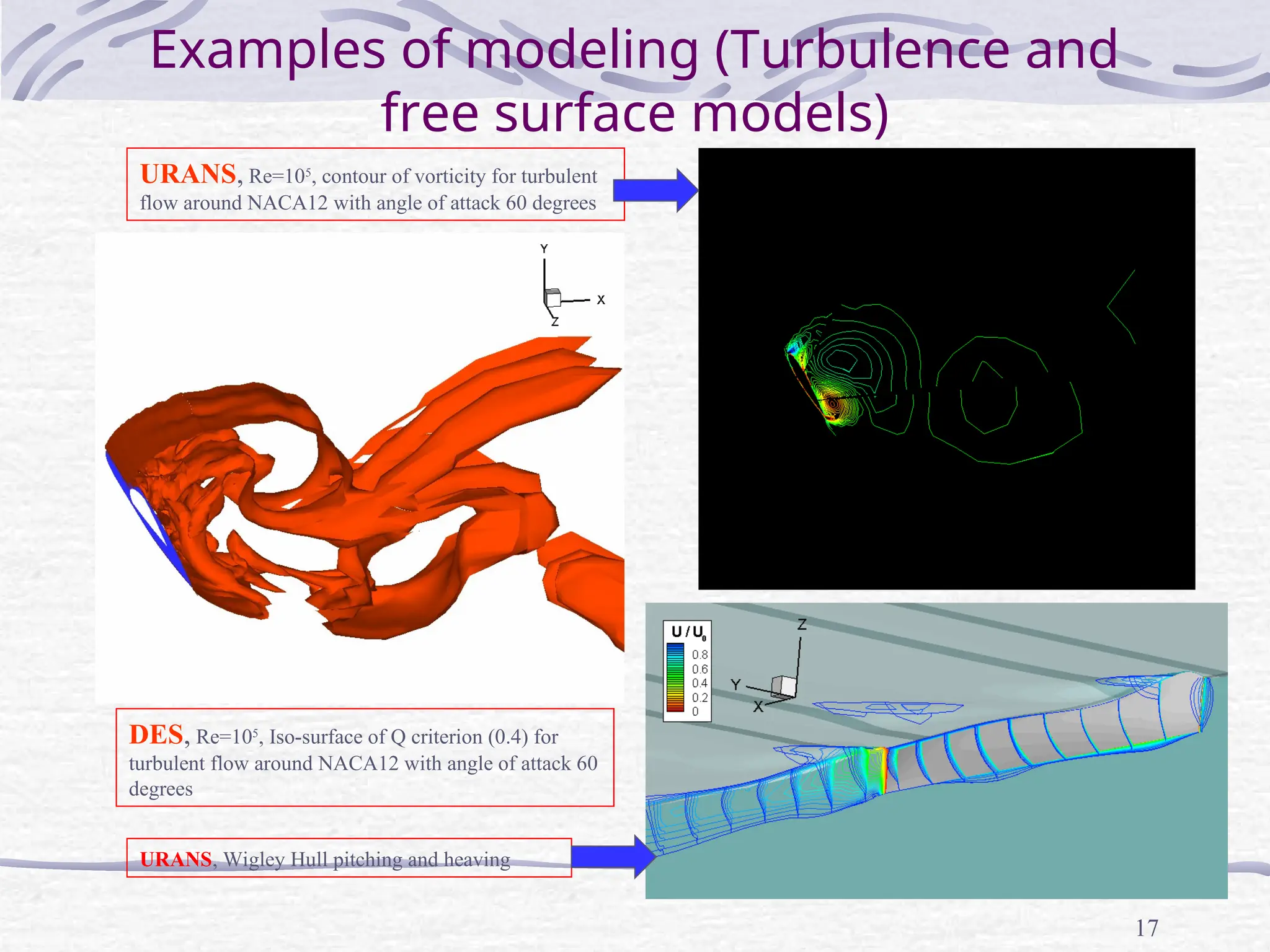
DES, Re=105
, Iso-surface of Q criterion (0.4) for
turbulent flow around NACA12 with angle of attack 60
degrees
URANS, Re=105
, contour of vorticity for turbulent
flow around NACA12 with angle of attack 60 degrees
URANS, Wigley Hull pitching and heaving

18. 18
Numerical methods
• The continuous Initial Boundary Value Problems
(IBVPs) are discretized into algebraic equations
using numerical methods. Assemble the system
of algebraic equations and solve the system to
get approximate solutions
• Numerical methods include:
1. Discretization methods
2. Solvers and numerical parameters
3. Grid generation and transformation
4. High Performance Computation (HPC) and post-
processing

19. 19
Discretization methods
• Finite difference methods (straightforward to apply,
usually for regular grid) and finite volumes and finite
element methods (usually for irregular meshes)
• Each type of methods above yields the same solution
if the grid is fine enough. However, some methods are
more suitable to some cases than others
• Finite difference methods for spatial derivatives with
different order of accuracies can be derived using
Taylor expansions, such as 2nd
order upwind scheme,
central differences schemes, etc.
• Higher order numerical methods usually predict
higher order of accuracy for CFD, but more likely
unstable due to less numerical dissipation
• Temporal derivatives can be integrated either by the
explicit method (Euler, Runge-Kutta, etc.) or implicit
method (e.g. Beam-Warming method)

20. 20
Discretization methods (Cont’d)
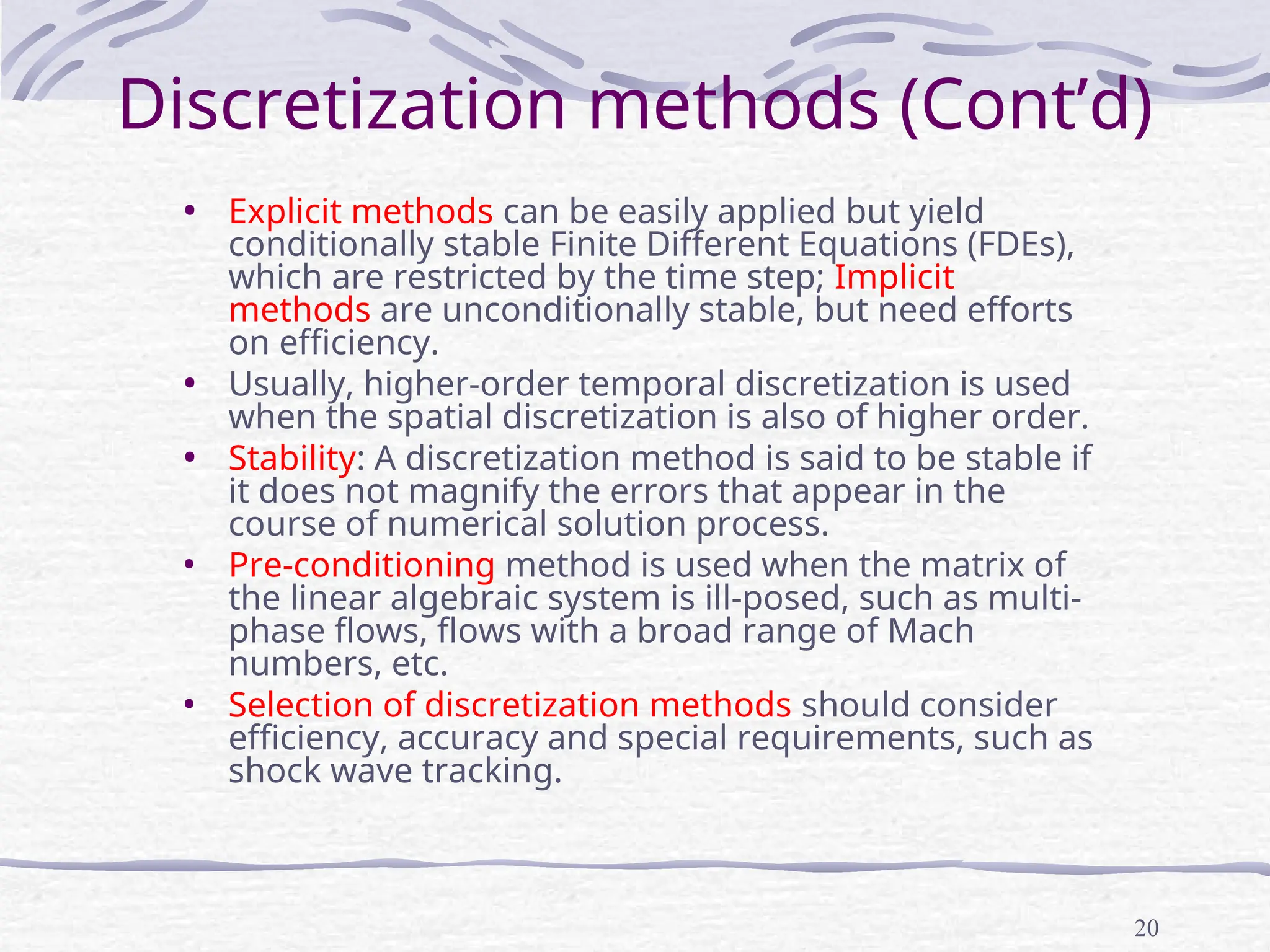
• Explicit methods can be easily applied but yield
conditionally stable Finite Different Equations (FDEs),
which are restricted by the time step; Implicit
methods are unconditionally stable, but need efforts
on efficiency.
• Usually, higher-order temporal discretization is used
when the spatial discretization is also of higher order.
• Stability: A discretization method is said to be stable if
it does not magnify the errors that appear in the
course of numerical solution process.
• Pre-conditioning method is used when the matrix of
the linear algebraic system is ill-posed, such as multi-
phase flows, flows with a broad range of Mach
numbers, etc.
• Selection of discretization methods should consider
efficiency, accuracy and special requirements, such as
shock wave tracking.

21. 21
Discretization methods
(example)
0






y
v
x
u
2
2
y
u
e
p
x
y
u
v
x
u
u



















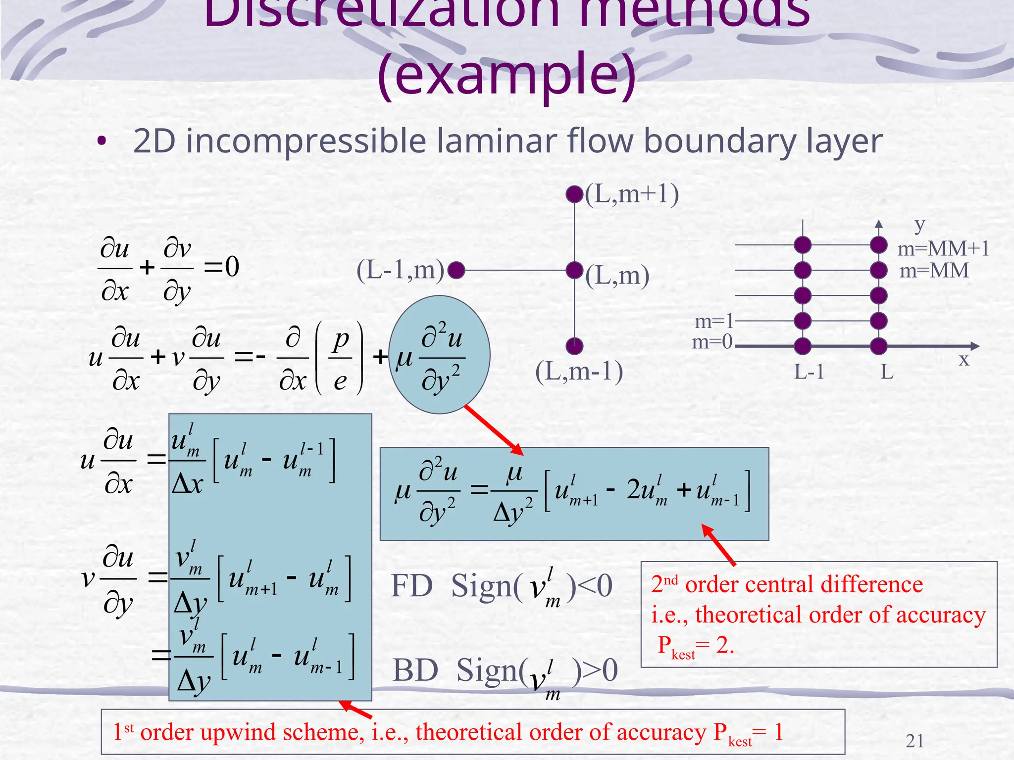
• 2D incompressible laminar flow boundary layer
m=0
m=1
L-1 L
y
x
m=MM
m=MM+1
(L,m-1)
(L,m)
(L,m+1)
(L-1,m)
1
l
l l
m
m m
u
u
u u u
x x


 
 
 
 
1
l
l l
m
m m
v
u
v u u
y y


 
 
 
 
1
l
l l
m
m m
v
u u
y

 
 
 

FD Sign( )<0
l
m
v
l
m
v
BD Sign( )>0
2
1 1
2 2
2
l l l
m m m
u
u u u
y y

  

 
  
 
 
2nd
order central difference
i.e., theoretical order of accuracy
Pkest= 2.
1st
order upwind scheme, i.e., theoretical order of accuracy Pkest= 1

22. 22
Discretization methods
(example)
1 1
2 2 2
1
2
1
l l l
l l l l
m m m
m m m m
FD
u v v
y
v u FD u BD u
x y y y y y
BD
y
  
 
 

     

     
     
     
     
 

 
1
( / )
l
l l
m
m m
u
u p e
x x
 
 
 
B2
B3 B1
B4
 
1
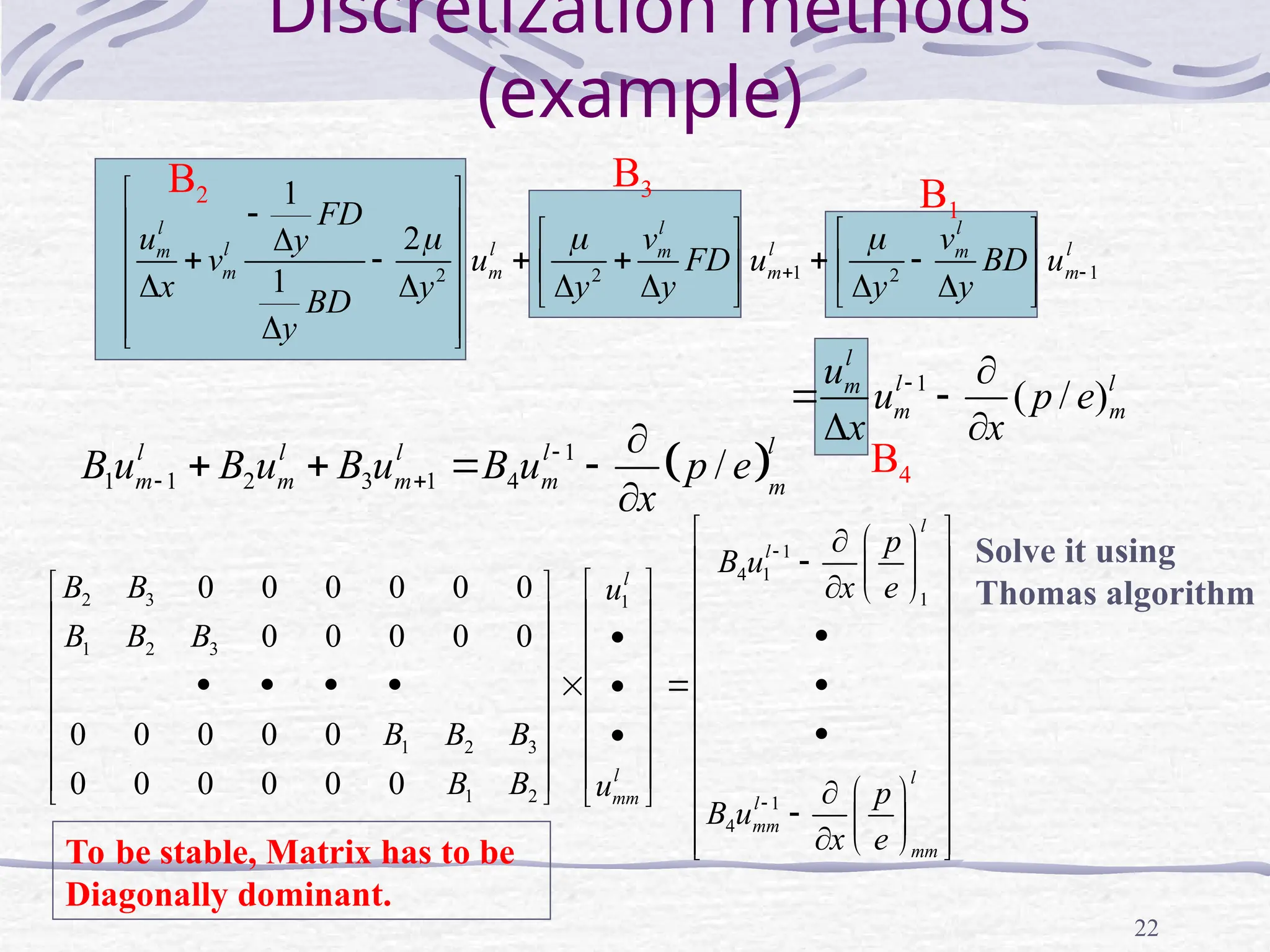
1 1 2 3 1 4 /
l
l l l l
m m m m m
B u B u B u B u p e
x

 

   

1
4 1
1
2 3 1
1 2 3
1 2 3
1 2 1
4
0 0 0 0 0 0
0 0 0 0 0
0 0 0 0 0
0 0 0 0 0 0
l
l
l
l l
mm l
mm
mm
p
B u
B B x e
u
B B B
B B B
B B u p
B u
x e


 
  

 
 

 
   
 
 
   


 
   
 
   
    
  
 
   


 
   
 
   
  
   

 
 

 
 
 
Solve it using
Thomas algorithm
To be stable, Matrix has to be
Diagonally dominant.

23. 23
Solvers and numerical parameters
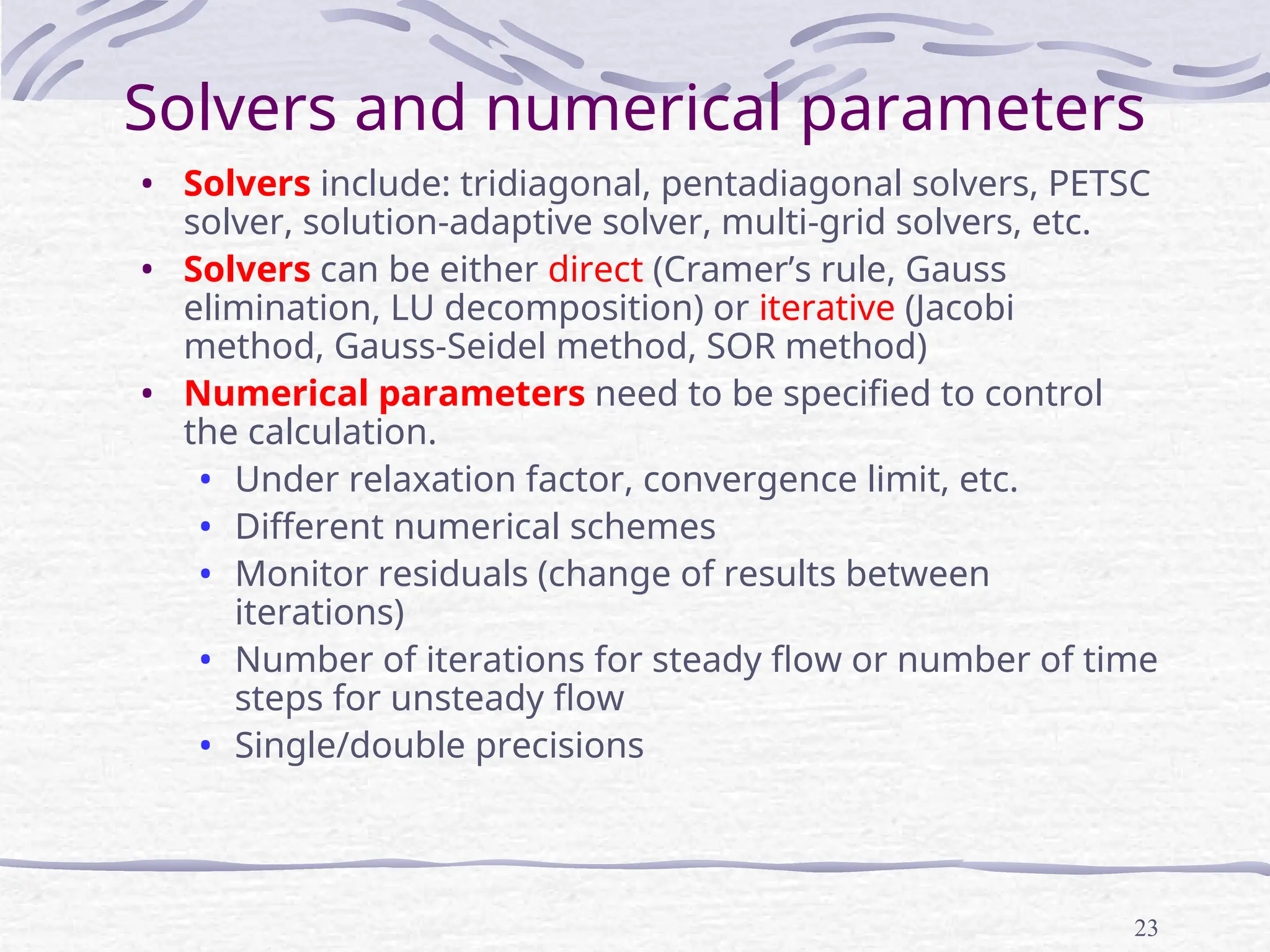
• Solvers include: tridiagonal, pentadiagonal solvers, PETSC
solver, solution-adaptive solver, multi-grid solvers, etc.
• Solvers can be either direct (Cramer’s rule, Gauss
elimination, LU decomposition) or iterative (Jacobi
method, Gauss-Seidel method, SOR method)
• Numerical parameters need to be specified to control
the calculation.
• Under relaxation factor, convergence limit, etc.
• Different numerical schemes
• Monitor residuals (change of results between
iterations)
• Number of iterations for steady flow or number of time
steps for unsteady flow
• Single/double precisions

24. 24
Numerical methods (grid
generation)
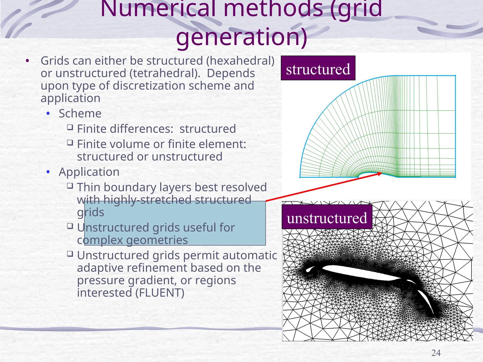
• Grids can either be structured (hexahedral)
or unstructured (tetrahedral). Depends
upon type of discretization scheme and
application
• Scheme
 Finite differences: structured
 Finite volume or finite element:
structured or unstructured
• Application
 Thin boundary layers best resolved
with highly-stretched structured
grids
 Unstructured grids useful for
complex geometries
 Unstructured grids permit automatic
adaptive refinement based on the
pressure gradient, or regions
interested (FLUENT)
structured
unstructured

25. 25
Numerical methods (grid
transformation)
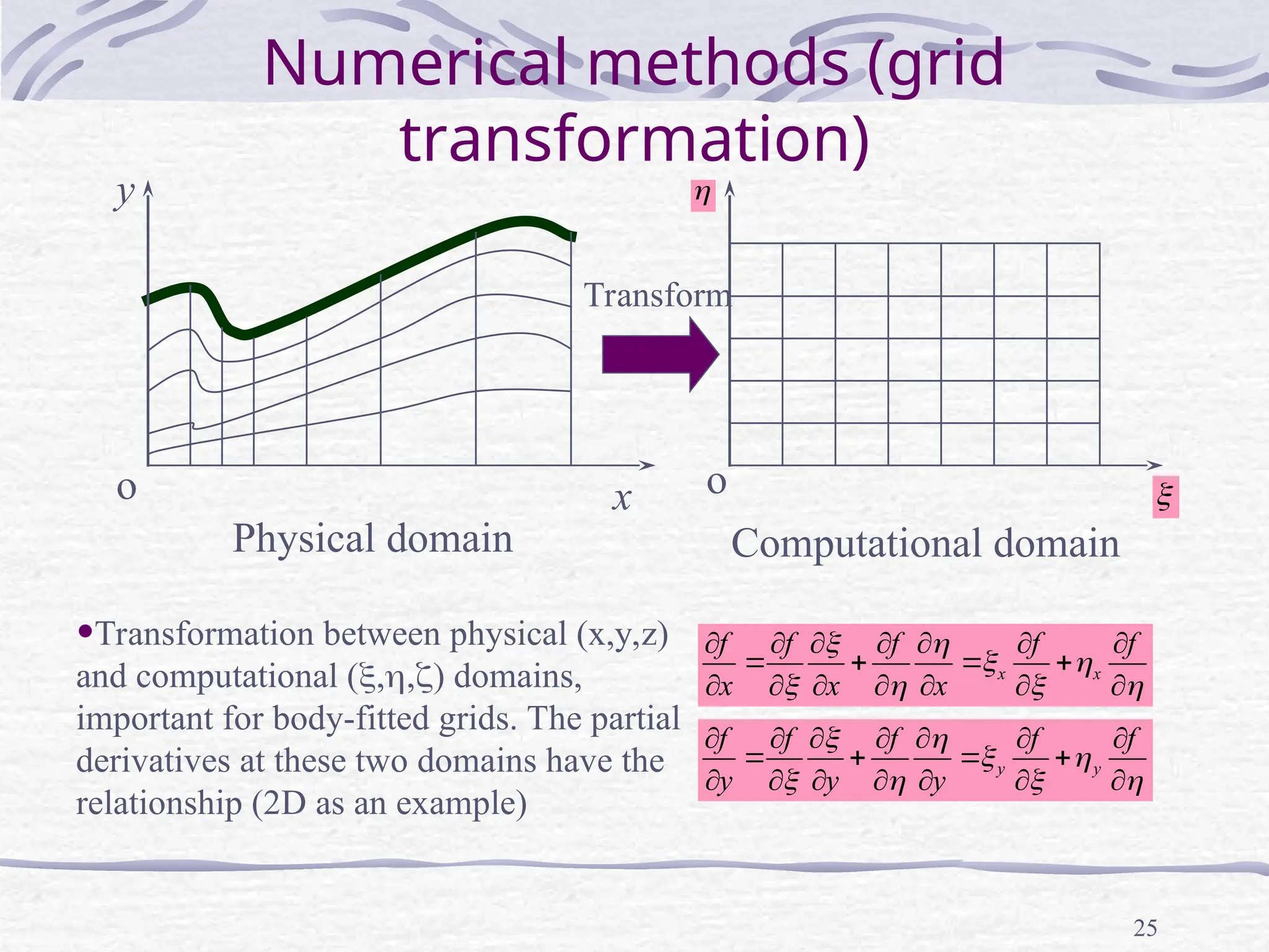
y
x
o o
Physical domain Computational domain
x x
f f f f f
x x x
 
 
   
      
   
      
y y
f f f f f
y y y
 
 
   
      
   
      
•Transformation between physical (x,y,z)
and computational () domains,
important for body-fitted grids. The partial
derivatives at these two domains have the
relationship (2D as an example)


Transform

26. 26
High performance computing
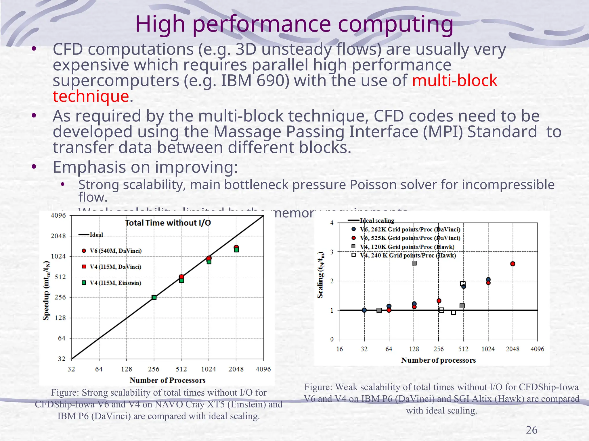
• CFD computations (e.g. 3D unsteady flows) are usually very
expensive which requires parallel high performance
supercomputers (e.g. IBM 690) with the use of multi-block
technique.
• As required by the multi-block technique, CFD codes need to be
developed using the Massage Passing Interface (MPI) Standard to
transfer data between different blocks.
• Emphasis on improving:
• Strong scalability, main bottleneck pressure Poisson solver for incompressible
flow.
• Weak scalability, limited by the memory requirements.
Figure: Strong scalability of total times without I/O for
CFDShip-Iowa V6 and V4 on NAVO Cray XT5 (Einstein) and
IBM P6 (DaVinci) are compared with ideal scaling.
Figure: Weak scalability of total times without I/O for CFDShip-Iowa
V6 and V4 on IBM P6 (DaVinci) and SGI Altix (Hawk) are compared
with ideal scaling.

27. 27
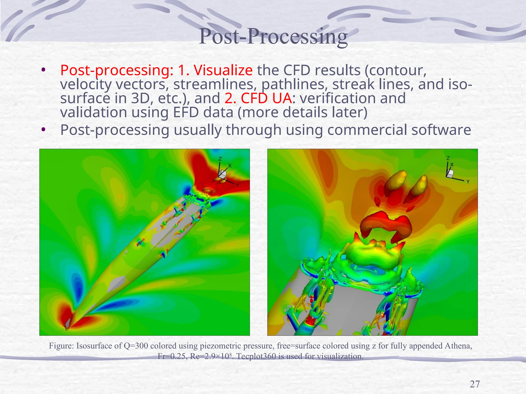
• Post-processing: 1. Visualize the CFD results (contour,
velocity vectors, streamlines, pathlines, streak lines, and iso-
surface in 3D, etc.), and 2. CFD UA: verification and
validation using EFD data (more details later)
• Post-processing usually through using commercial software
Post-Processing
Figure: Isosurface of Q=300 colored using piezometric pressure, free=surface colored using z for fully appended Athena,
Fr=0.25, Re=2.9×108
. Tecplot360 is used for visualization.

28. 28
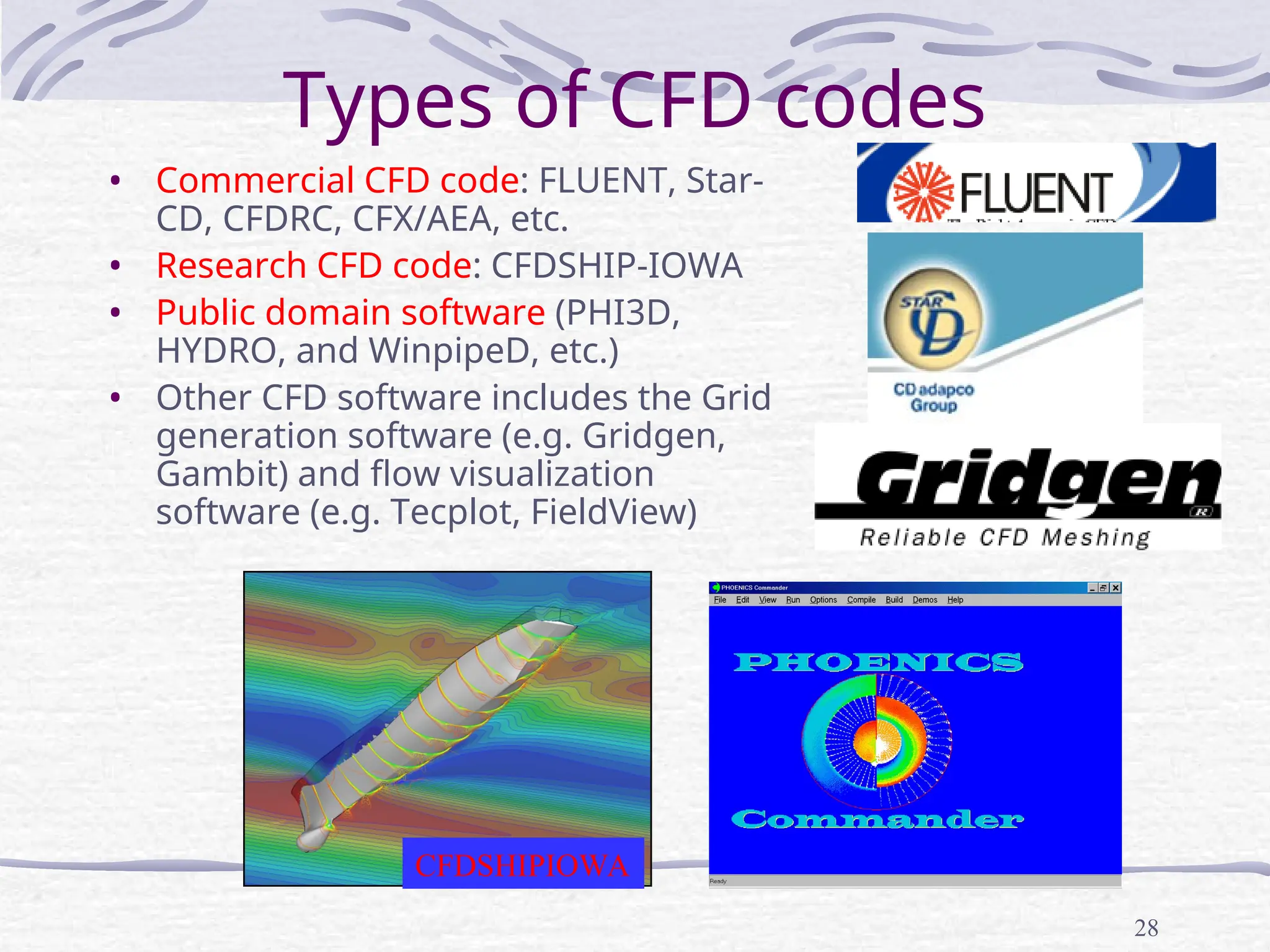
Types of CFD codes
• Commercial CFD code: FLUENT, Star-
CD, CFDRC, CFX/AEA, etc.
• Research CFD code: CFDSHIP-IOWA
• Public domain software (PHI3D,
HYDRO, and WinpipeD, etc.)
• Other CFD software includes the Grid
generation software (e.g. Gridgen,
Gambit) and flow visualization
software (e.g. Tecplot, FieldView)
CFDSHIPIOWA

29. 29
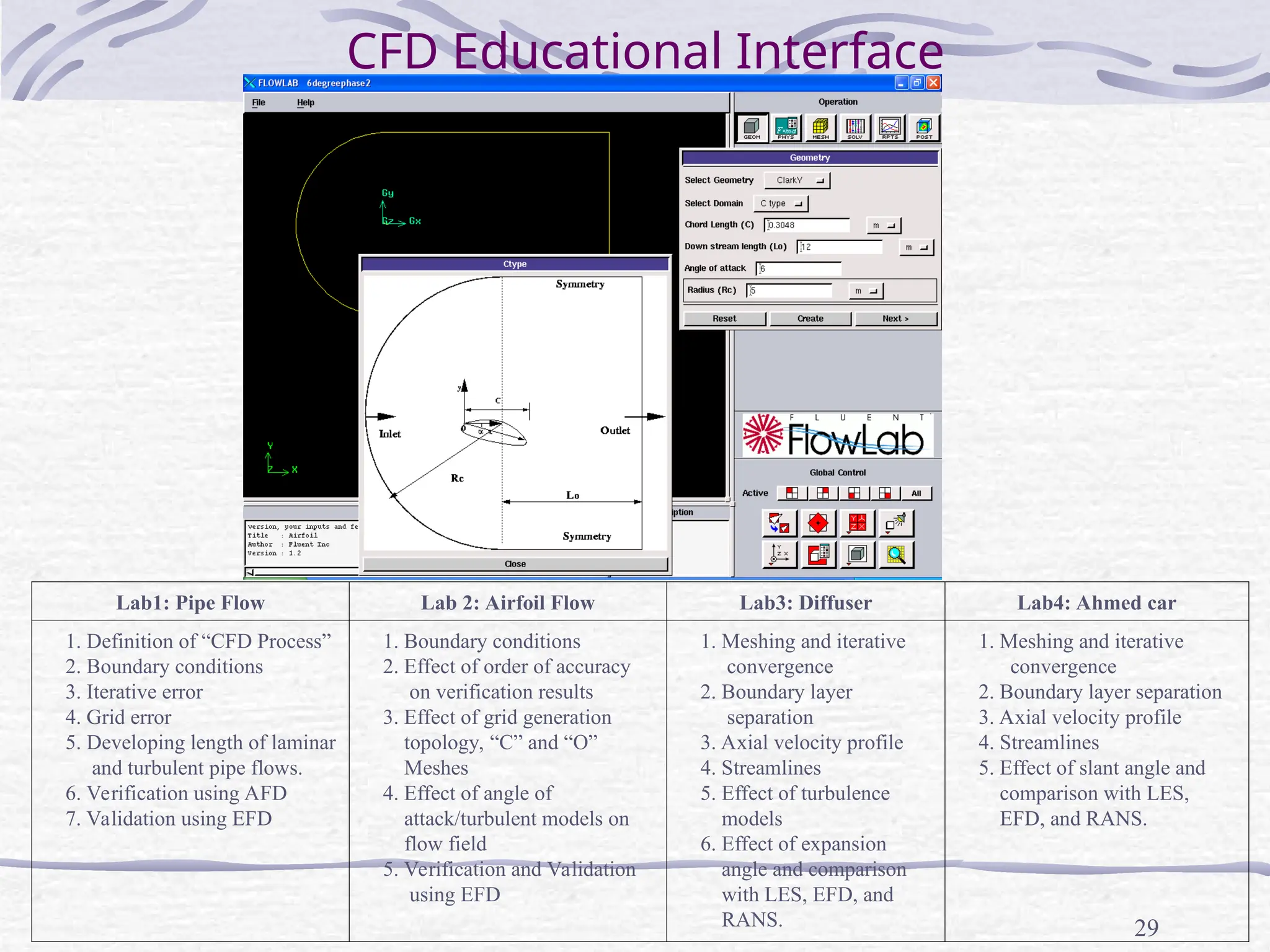
CFD Educational Interface
Lab1: Pipe Flow Lab 2: Airfoil Flow Lab3: Diffuser Lab4: Ahmed car
1. Definition of “CFD Process”
2. Boundary conditions
3. Iterative error
4. Grid error
5. Developing length of laminar
and turbulent pipe flows.
6. Verification using AFD
7. Validation using EFD
1. Boundary conditions
2. Effect of order of accuracy
on verification results
3. Effect of grid generation
topology, “C” and “O”
Meshes
4. Effect of angle of
attack/turbulent models on
flow field
5. Verification and Validation
using EFD
1. Meshing and iterative
convergence
2. Boundary layer
separation
3. Axial velocity profile
4. Streamlines
5. Effect of turbulence
models
6. Effect of expansion
angle and comparison
with LES, EFD, and
RANS.
1. Meshing and iterative
convergence
2. Boundary layer separation
3. Axial velocity profile
4. Streamlines
5. Effect of slant angle and
comparison with LES,
EFD, and RANS.

30. 30
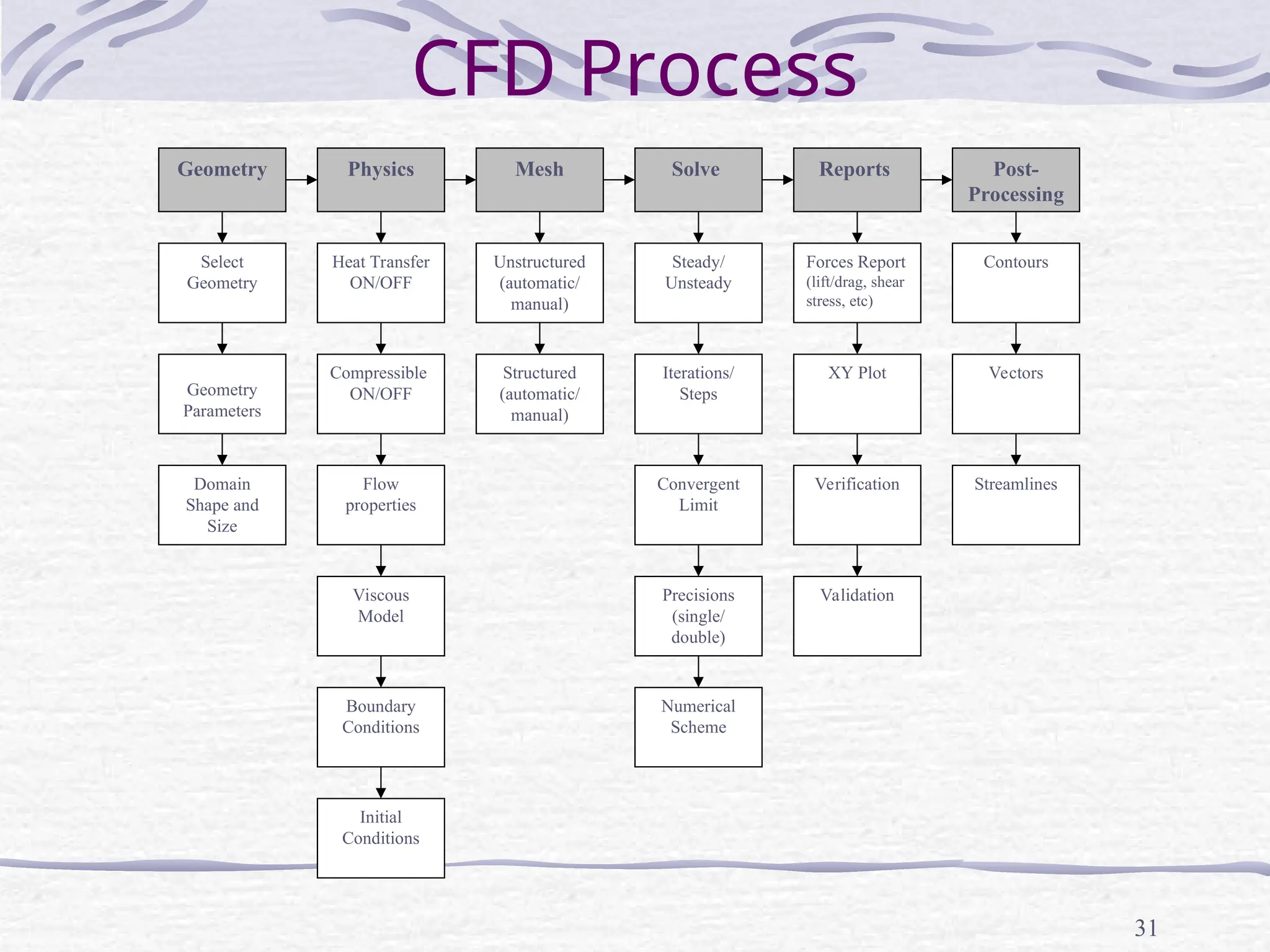
CFD process
• Purposes of CFD codes will be different for different
applications: investigation of bubble-fluid interactions for
bubbly flows, study of wave induced massively separated
flows for free-surface, etc.
• Depend on the specific purpose and flow conditions of the
problem, different CFD codes can be chosen for different
applications (aerospace, marines, combustion, multi-phase
flows, etc.)
• Once purposes and CFD codes chosen, “CFD process” is the
steps to set up the IBVP problem and run the code:
1. Geometry
2. Physics
3. Mesh
4. Solve
5. Reports
6. Post processing

31. 31
CFD Process
Viscous
Model
Boundary
Conditions
Initial
Conditions
Convergent
Limit
Contours
Precisions
(single/
double)
Numerical
Scheme
Vectors
Streamlines
Verification
Geometry
Select
Geometry
Geometry
Parameters
Physics Mesh Solve Post-
Processing
Compressible
ON/OFF
Flow
properties
Unstructured
(automatic/
manual)
Steady/
Unsteady
Forces Report
(lift/drag, shear
stress, etc)
XY Plot
Domain
Shape and
Size
Heat Transfer
ON/OFF
Structured
(automatic/
manual)
Iterations/
Steps
Validation
Reports

32. 32
Geometry
• Selection of an appropriate coordinate
• Determine the domain size and shape
• Any simplifications needed?
• What kinds of shapes needed to be used to best
resolve the geometry? (lines, circular, ovals, etc.)
• For commercial code, geometry is usually created
using commercial software (either separated from
the commercial code itself, like Gambit, or
combined together, like FlowLab)
• For research code, commercial software (e.g.
Gridgen) is used.

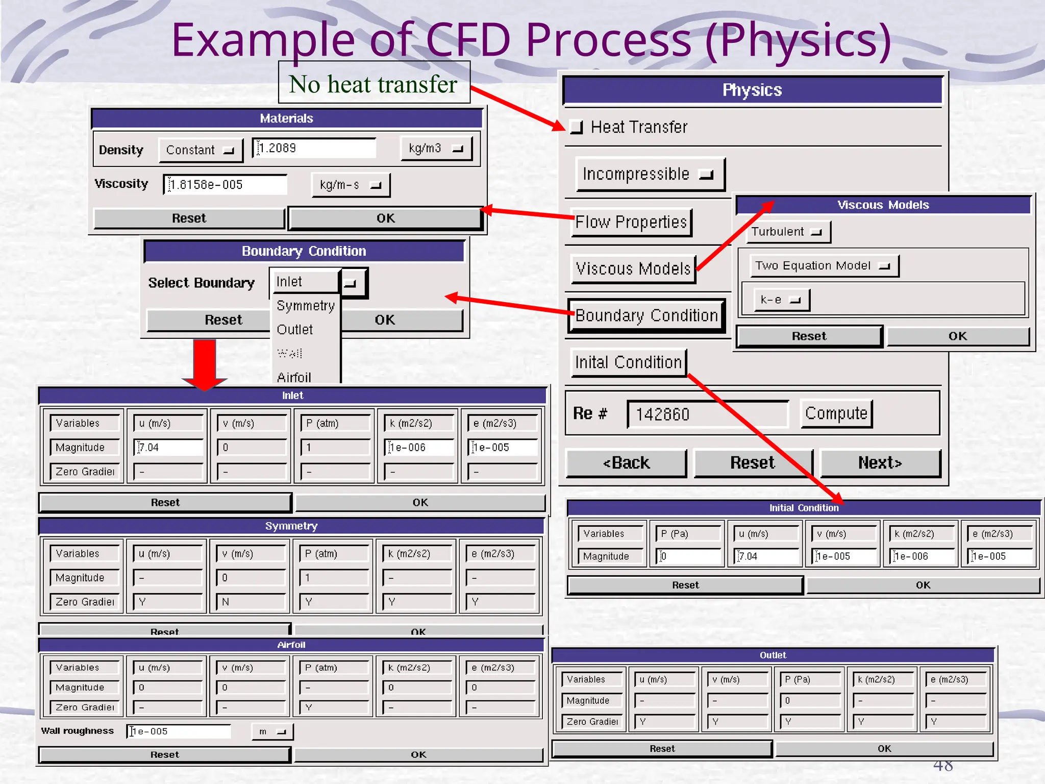
33. 33
Physics
• Flow conditions and fluid properties
1. Flow conditions: inviscid, viscous, laminar, or
turbulent, etc.
2. Fluid properties: density, viscosity, and
thermal conductivity, etc.
3. Flow conditions and properties usually
presented in dimensional form in industrial
commercial CFD software, whereas in non-
dimensional variables for research codes.
• Selection of models: different models usually
fixed by codes, options for user to choose
• Initial and Boundary Conditions: not fixed
by codes, user needs specify them for different
applications.

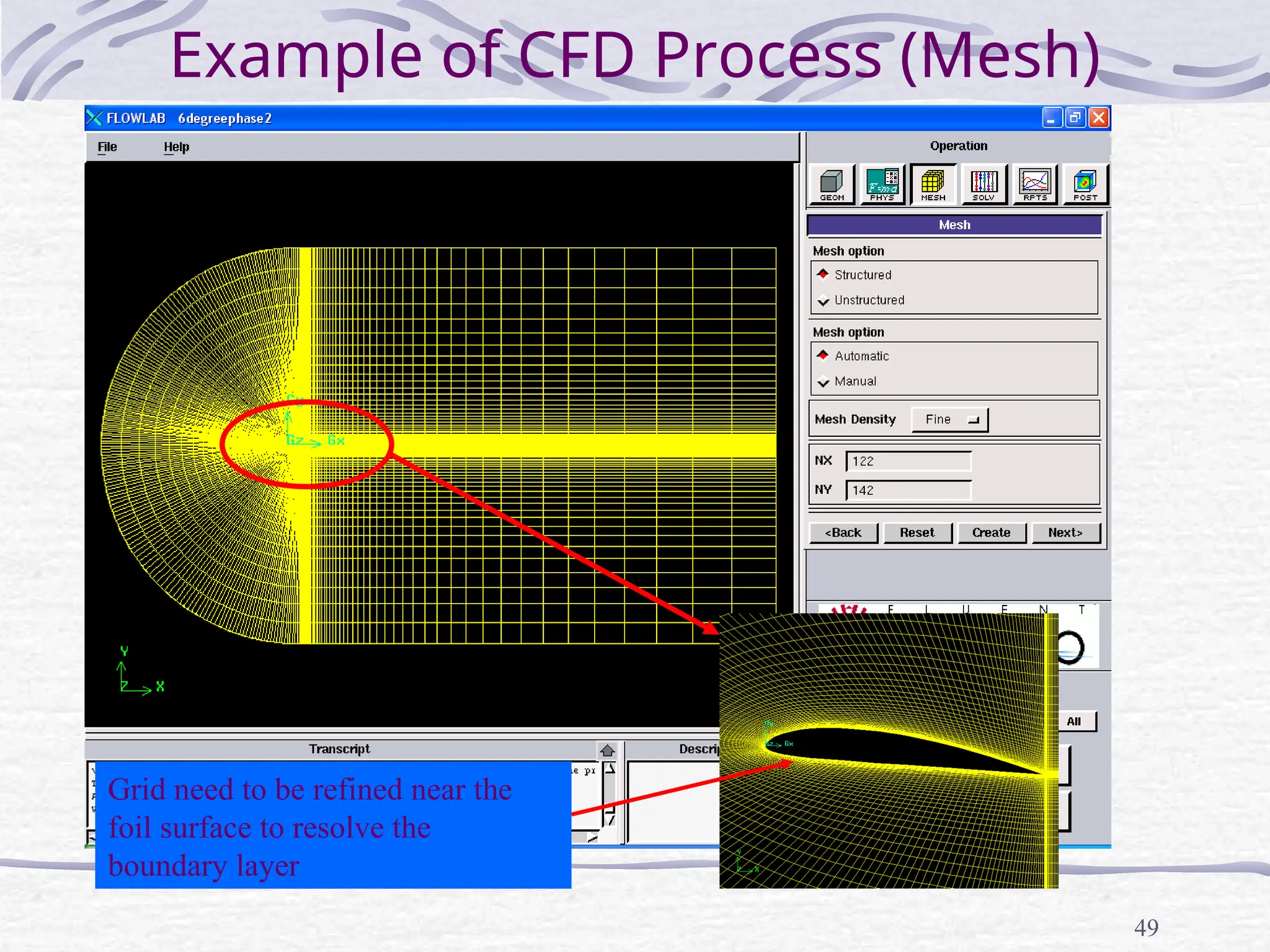
34. 34
Mesh
• Meshes should be well designed to resolve
important flow features which are dependent upon
flow condition parameters (e.g., Re), such as the
grid refinement inside the wall boundary layer
• Mesh can be generated by either commercial codes
(Gridgen, Gambit, etc.) or research code (using
algebraic vs. PDE based, conformal mapping, etc.)
• The mesh, together with the boundary conditions
need to be exported from commercial software in a
certain format that can be recognized by the
research CFD code or other commercial CFD
software.

35. 35
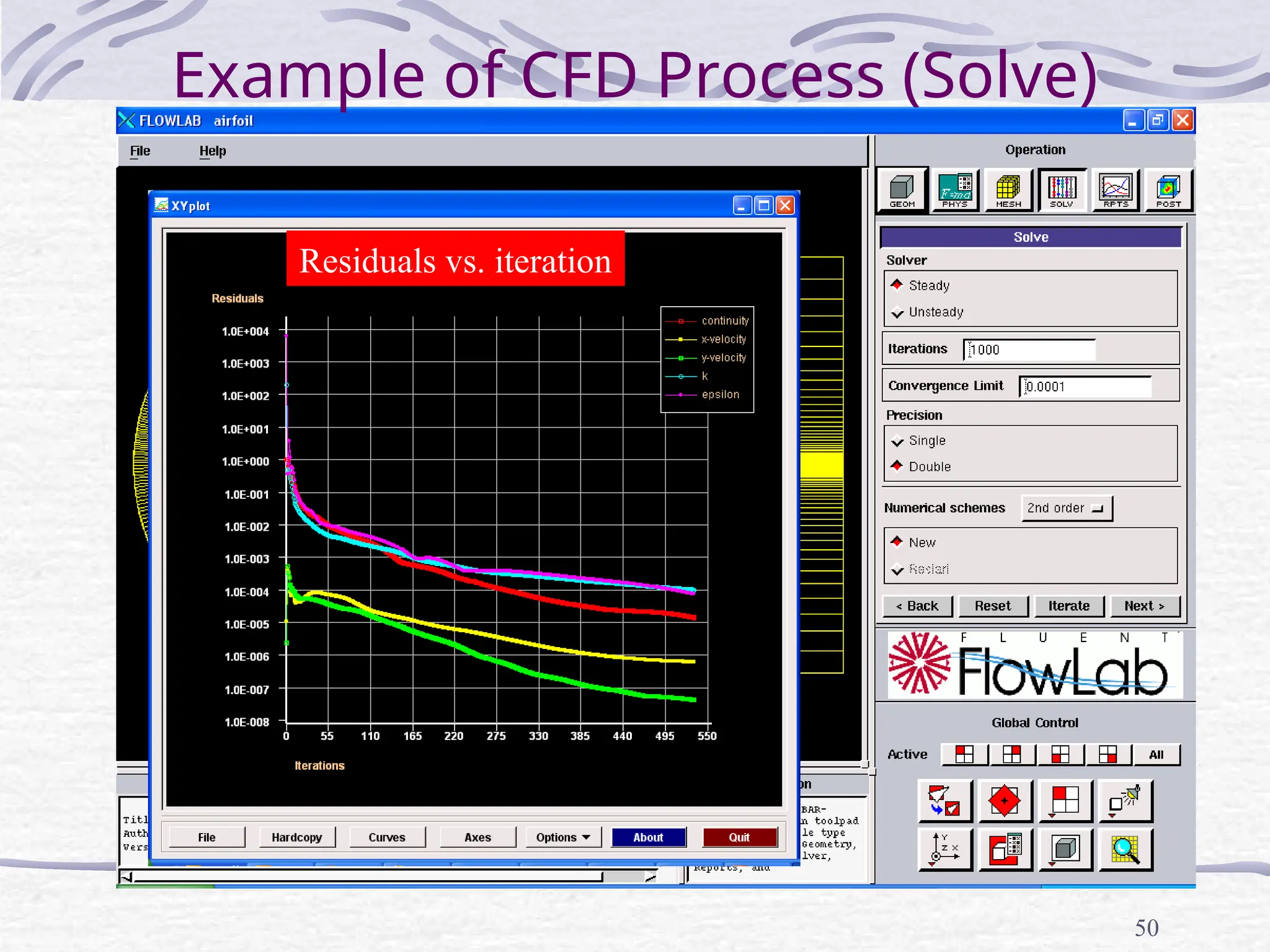
Solve
• Setup appropriate numerical parameters
• Choose appropriate Solvers
• Solution procedure (e.g. incompressible flows)
Solve the momentum, pressure Poisson
equations and get flow field quantities, such
as velocity, turbulence intensity, pressure
and integral quantities (lift, drag forces)

36. 36
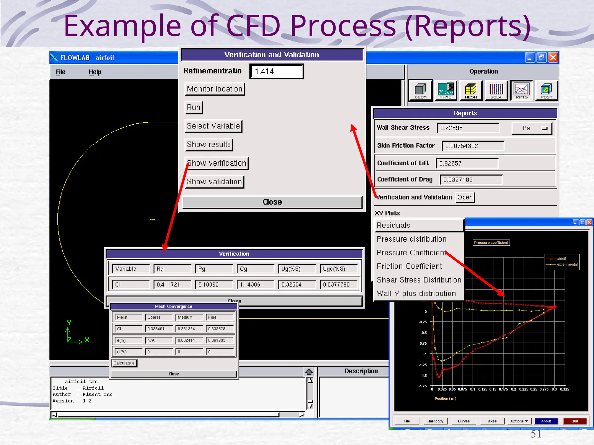
Reports
• Reports saved the time history of the
residuals of the velocity, pressure and
temperature, etc.
• Report the integral quantities, such as total
pressure drop, friction factor (pipe flow), lift
and drag coefficients (airfoil flow), etc.
• XY plots could present the centerline
velocity/pressure distribution, friction factor
distribution (pipe flow), pressure coefficient
distribution (airfoil flow).
• AFD or EFD data can be imported and put on
top of the XY plots for validation

37. 37
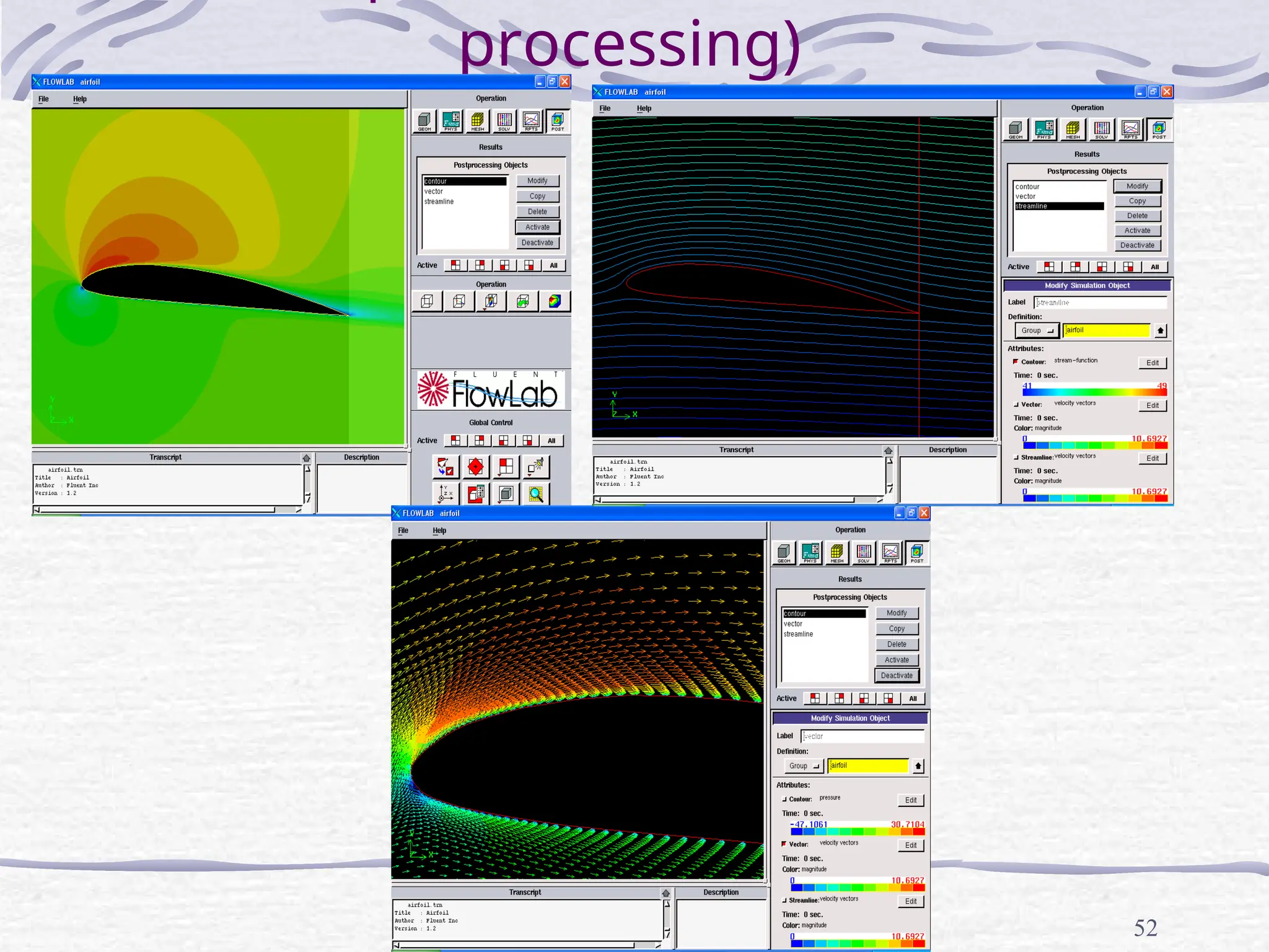
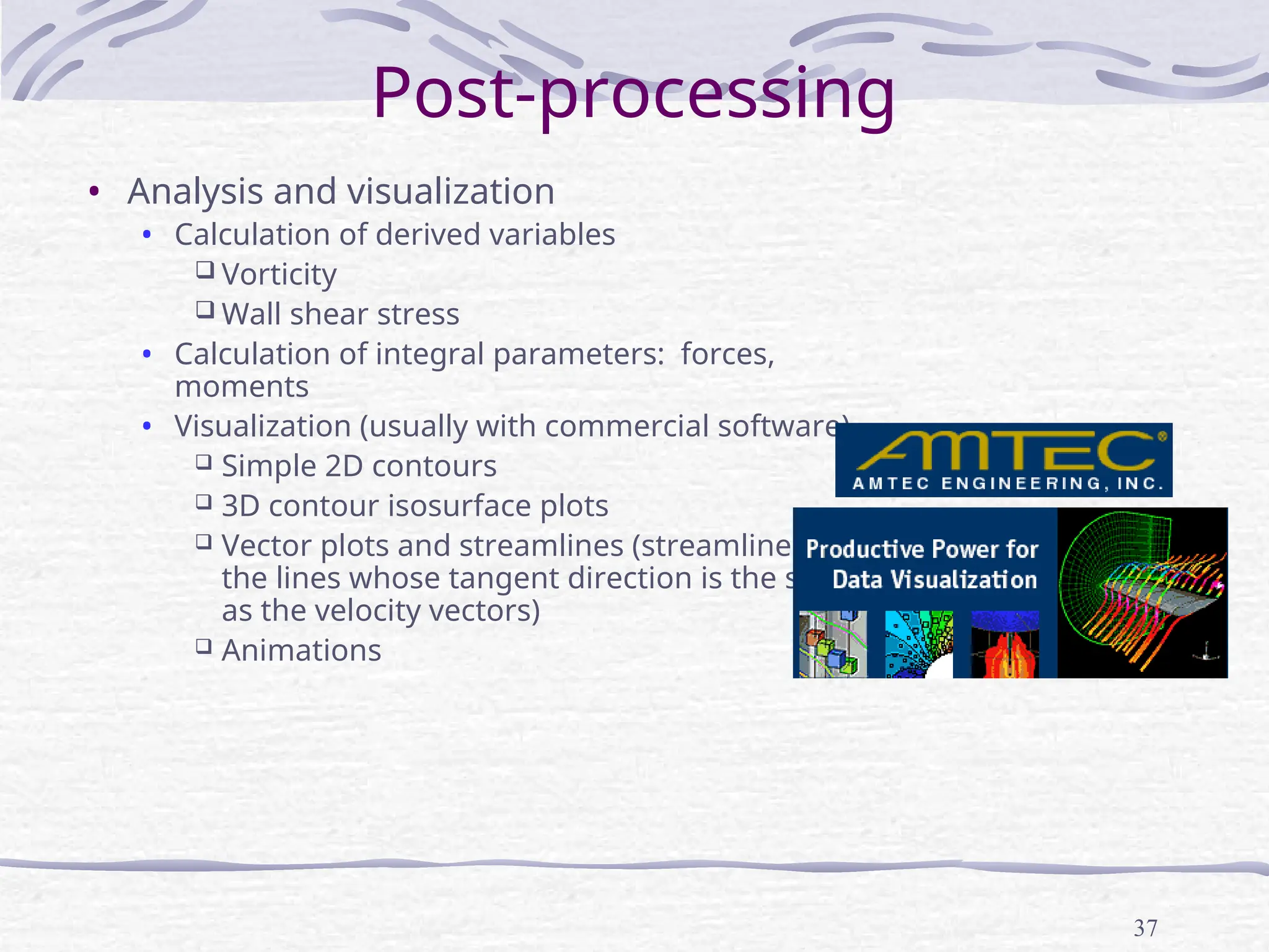
Post-processing
• Analysis and visualization
• Calculation of derived variables
 Vorticity
 Wall shear stress
• Calculation of integral parameters: forces,
moments
• Visualization (usually with commercial software)
 Simple 2D contours
 3D contour isosurface plots
 Vector plots and streamlines (streamlines are
the lines whose tangent direction is the same
as the velocity vectors)
 Animations

38. 38
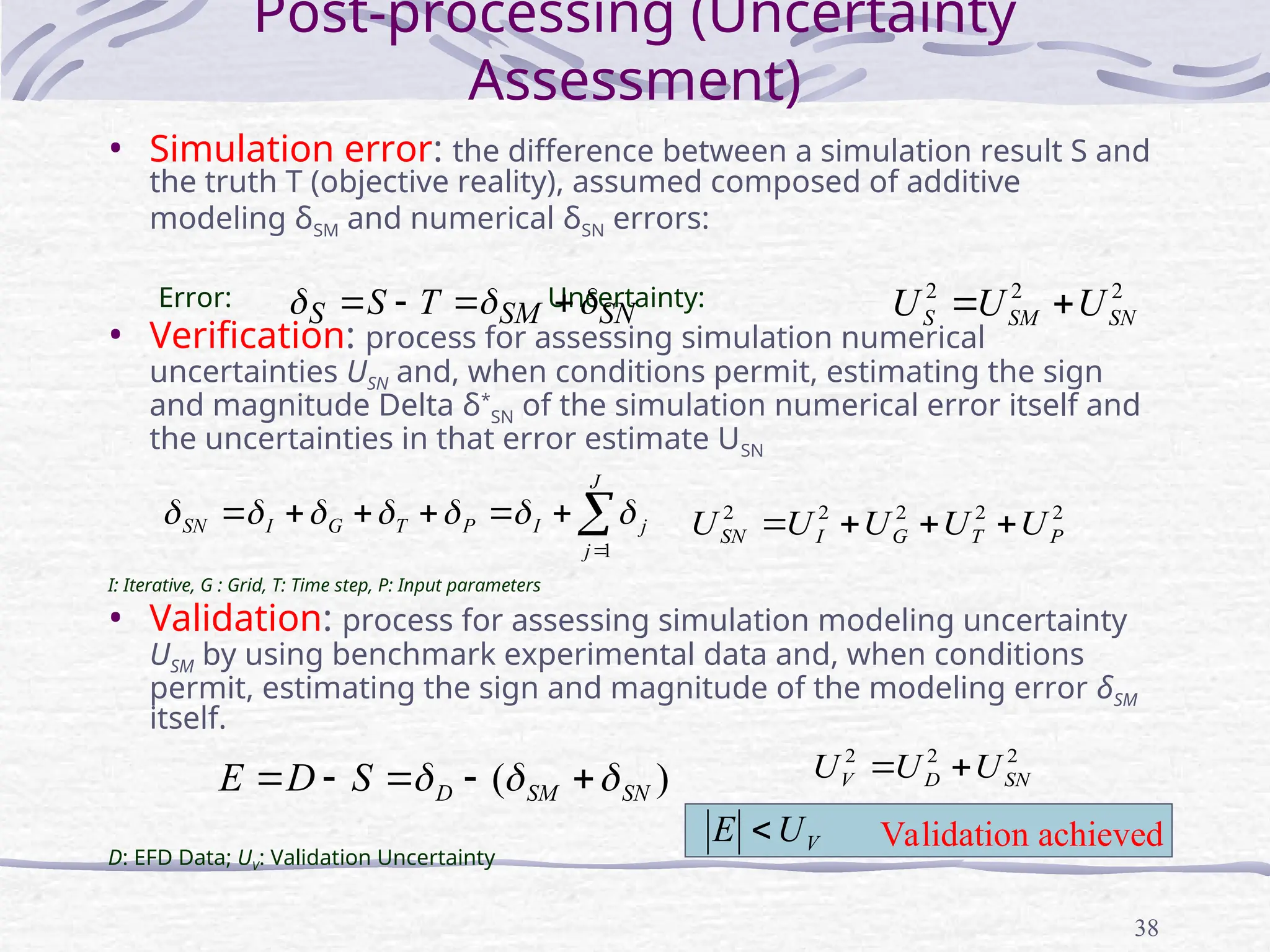
Post-processing (Uncertainty
Assessment)
• Simulation error: the difference between a simulation result S and
the truth T (objective reality), assumed composed of additive
modeling δSM and numerical δSN errors:
Error: Uncertainty:
• Verification: process for assessing simulation numerical
uncertainties USN and, when conditions permit, estimating the sign
and magnitude Delta δ*
SN of the simulation numerical error itself and
the uncertainties in that error estimate USN
I: Iterative, G : Grid, T: Time step, P: Input parameters
• Validation: process for assessing simulation modeling uncertainty
USM by using benchmark experimental data and, when conditions
permit, estimating the sign and magnitude of the modeling error δSM
itself.
D: EFD Data; UV: Validation Uncertainty
SN
SM
S T
S 

 


 2
2
2
SN
SM
S U
U
U 









J
j
j
I
P
T
G
I
SN
1






 2
2
2
2
2
P
T
G
I
SN U
U
U
U
U 



)
( SN
SM
D
S
D
E 

 




2
2
2
SN
D
V U
U
U 

V
U
E  Validation achieved

39. 39
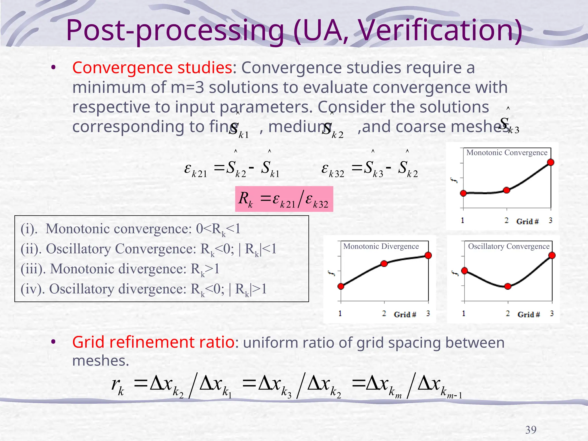
Post-processing (UA, Verification)
• Convergence studies: Convergence studies require a
minimum of m=3 solutions to evaluate convergence with
respective to input parameters. Consider the solutions
corresponding to fine , medium ,and coarse meshes
1
k
S

2
k
S

3
k
S

(i). Monotonic convergence: 0<Rk<1
(ii). Oscillatory Convergence: Rk<0; | Rk|<1
(iii). Monotonic divergence: Rk>1
(iv). Oscillatory divergence: Rk<0; | Rk|>1
21 2 1
k k k
S S

 
  32 3 2
k k k
S S

 
 
21 32
k k k
R  

• Grid refinement ratio: uniform ratio of grid spacing between
meshes.
1
2
3
1
2 








 m
m k
k
k
k
k
k
k x
x
x
x
x
x
r
Monotonic Convergence
Monotonic Divergence Oscillatory Convergence

40. 40
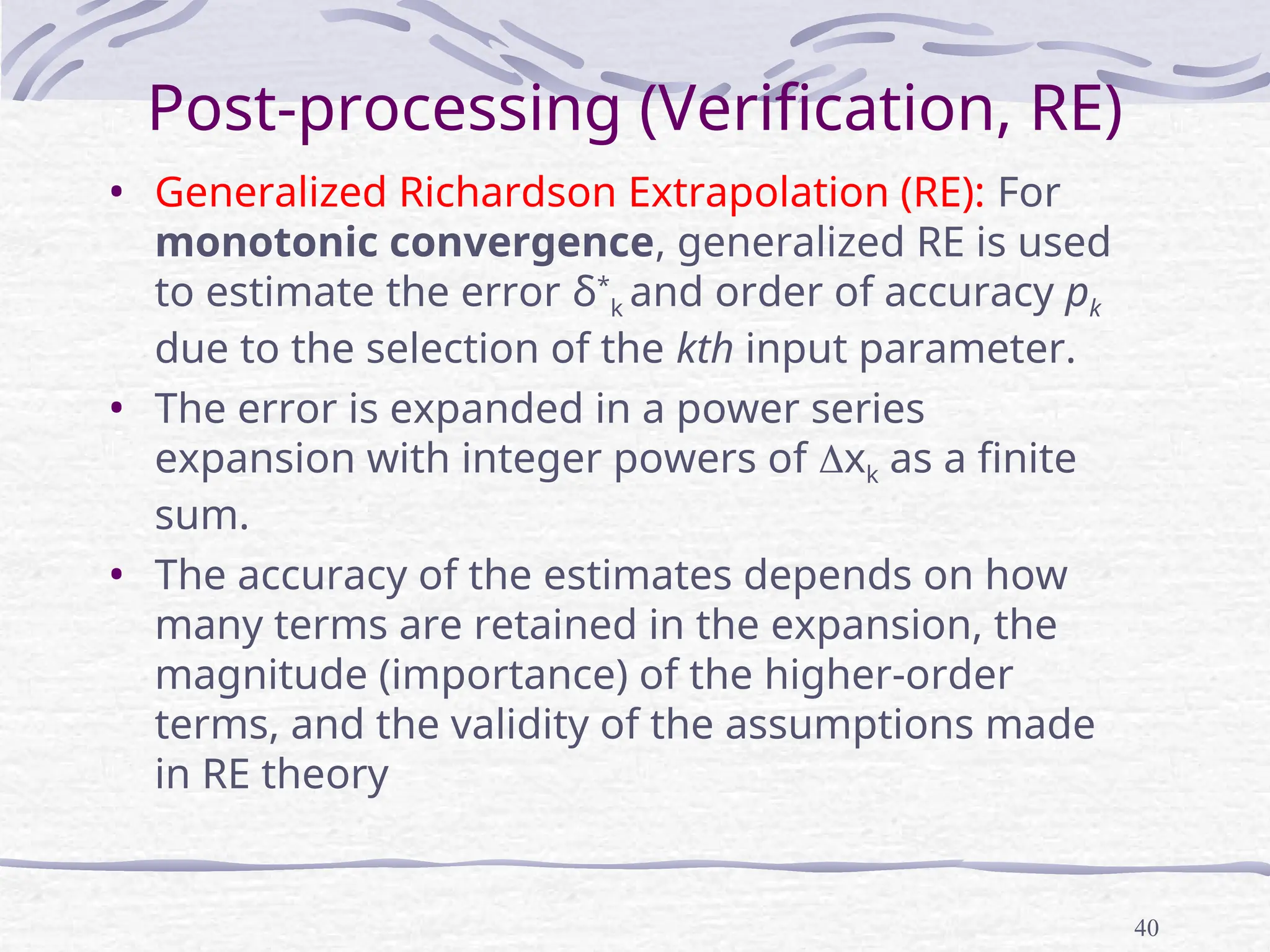
Post-processing (Verification, RE)
• Generalized Richardson Extrapolation (RE): For
monotonic convergence, generalized RE is used
to estimate the error δ*
k and order of accuracy pk
due to the selection of the kth input parameter.
• The error is expanded in a power series
expansion with integer powers of xk as a finite
sum.
• The accuracy of the estimates depends on how
many terms are retained in the expansion, the
magnitude (importance) of the higher-order
terms, and the validity of the assumptions made
in RE theory

41. 41
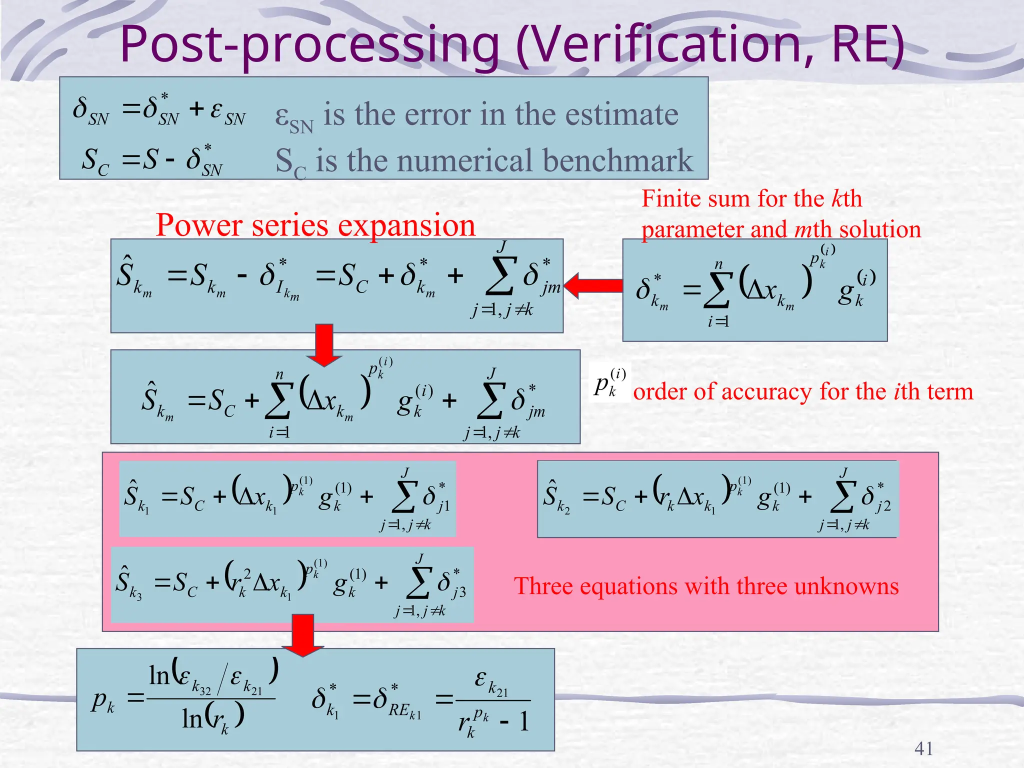
Post-processing (Verification, RE)
)
(i
k
p
 
 
 
i
k
p
n
i
k
k g
x
i
k
m
m 



1
*

1
21
1
1
*
*


 k
k p
k
k
RE
k
r



 
 
k
k
k
k
r
p
ln
ln 21
32










J
k
j
j
jm
k
C
I
k
k m
m
k
m
m
S
S
S
,
1
*
*
*
ˆ 


  
 






J
k
j
j
jm
i
k
p
n
i
k
C
k g
x
S
S
i
k
m
m
,
1
*
)
(
1
)
(
ˆ 
Power series expansion
Finite sum for the kth
parameter and mth solution
order of accuracy for the ith term
Three equations with three unknowns
  





J
k
j
j
j
k
p
k
C
k g
x
S
S k
,
1
*
1
)
1
(
)
1
(
1
1
ˆ 
  





J
k
j
j
j
k
p
k
k
C
k g
x
r
S
S k
,
1
*
3
)
1
(
2
)
1
(
1
3
ˆ 
  





J
k
j
j
j
k
p
k
k
C
k g
x
r
S
S k
,
1
*
2
)
1
(
)
1
(
1
2
ˆ 
SN
SN
SN 

 
 *
*
SN
C S
S 


εSN is the error in the estimate
SC is the numerical benchmark

42. 42
Post-processing (UA, Verification, cont’d)
• Monotonic Convergence: Generalized Richardson
Extrapolation
 
 
 








*
1
2
*
1
1
.
0
1
4
.
2
1
1
k
RE
k
k
RE
k
C
C
kc
U


• Oscillatory Convergence: Uncertainties can be estimated, but without
signs and magnitudes of the errors.
• Divergence
 
L
U
k S
S
U 

2
1
1. Correction
factors
2. GCI approach *
1
k
RE
s
k F
U 
   *
1
1 k
RE
s
kc F
U 


 
 
32 21
ln
ln
k k
k
k
p
r
 

1
1
k
kest
p
k
k p
k
r
C
r



1
* 21
1
k k
k
RE p
k
r

 

  1
1
2 *
*
9.6 1 1.1
2 1 1
k
k
k RE
k
k RE
C
U
C


 
 
 

   
  

1 0.125
k
C
 
1 0.125
k
C
 
1 0.25
k
C
 
25
.
0
|
1
| 
 k
C
|
|
|]
1
[| *
1
k
RE
k
C 

• In this course, only grid uncertainties studied. So, all the variables with
subscribe symbol k will be replaced by g, such as “Uk” will be “Ug”
est
k
p is the theoretical order of accuracy, 2 for 2nd
order and 1 for 1st
order schemes k
U is the uncertainties based on fine mesh
solution, is the uncertainties based on
numerical benchmark SC
kc
U
is the correction factor
k
C
FS: Factor of Safety

43. 43
• Asymptotic Range: For sufficiently small xk, the
solutions are in the asymptotic range such that
higher-order terms are negligible and the
assumption that and are independent of
xk is valid.
• When Asymptotic Range reached, will be close
to the theoretical value , and the correction
factor
will be close to 1.
• To achieve the asymptotic range for practical
geometry and conditions is usually not possible
and number of grids m>3 is undesirable from a
resources point of view
Post-processing (Verification,
Asymptotic Range)
 
i
k
p
 
i
k
g
est
k
p
k
p
k
C

44. 44
Post-processing (UA, Verification,
cont’d)
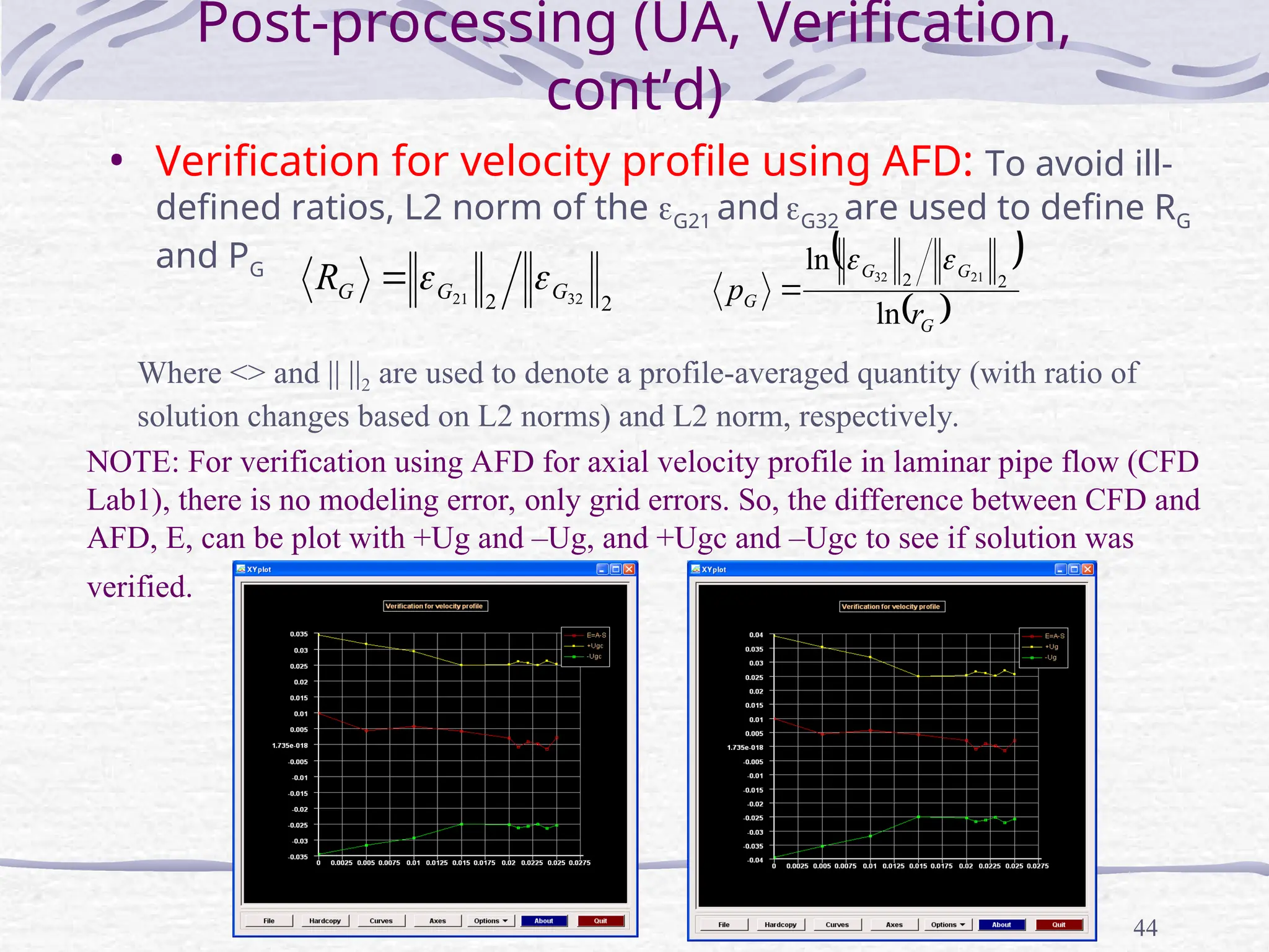
• Verification for velocity profile using AFD: To avoid ill-
defined ratios, L2 norm of the G21 and G32 are used to define RG
and PG
2
2 32
21 G
G
G
R 


NOTE: For verification using AFD for axial velocity profile in laminar pipe flow (CFD
Lab1), there is no modeling error, only grid errors. So, the difference between CFD and
AFD, E, can be plot with +Ug and –Ug, and +Ugc and –Ugc to see if solution was
verified.
 
 
G
G
G
G
r
p
ln
ln
2
2 21
32



Where <> and || ||2 are used to denote a profile-averaged quantity (with ratio of
solution changes based on L2 norms) and L2 norm, respectively.

45. 45
Post-processing (Verification: Iterative
Convergence)
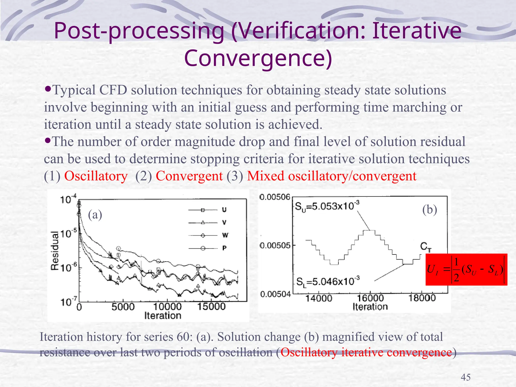
•Typical CFD solution techniques for obtaining steady state solutions
involve beginning with an initial guess and performing time marching or
iteration until a steady state solution is achieved.
•The number of order magnitude drop and final level of solution residual
can be used to determine stopping criteria for iterative solution techniques
(1) Oscillatory (2) Convergent (3) Mixed oscillatory/convergent
Iteration history for series 60: (a). Solution change (b) magnified view of total
resistance over last two periods of oscillation (Oscillatory iterative convergence)
(b)
(a)
)
(
2
1
L
U
I S
S
U 


46. 46
Post-processing (UA, Validation)
V
U
E 
E
UV 
Validation achieved
Validation not achieved
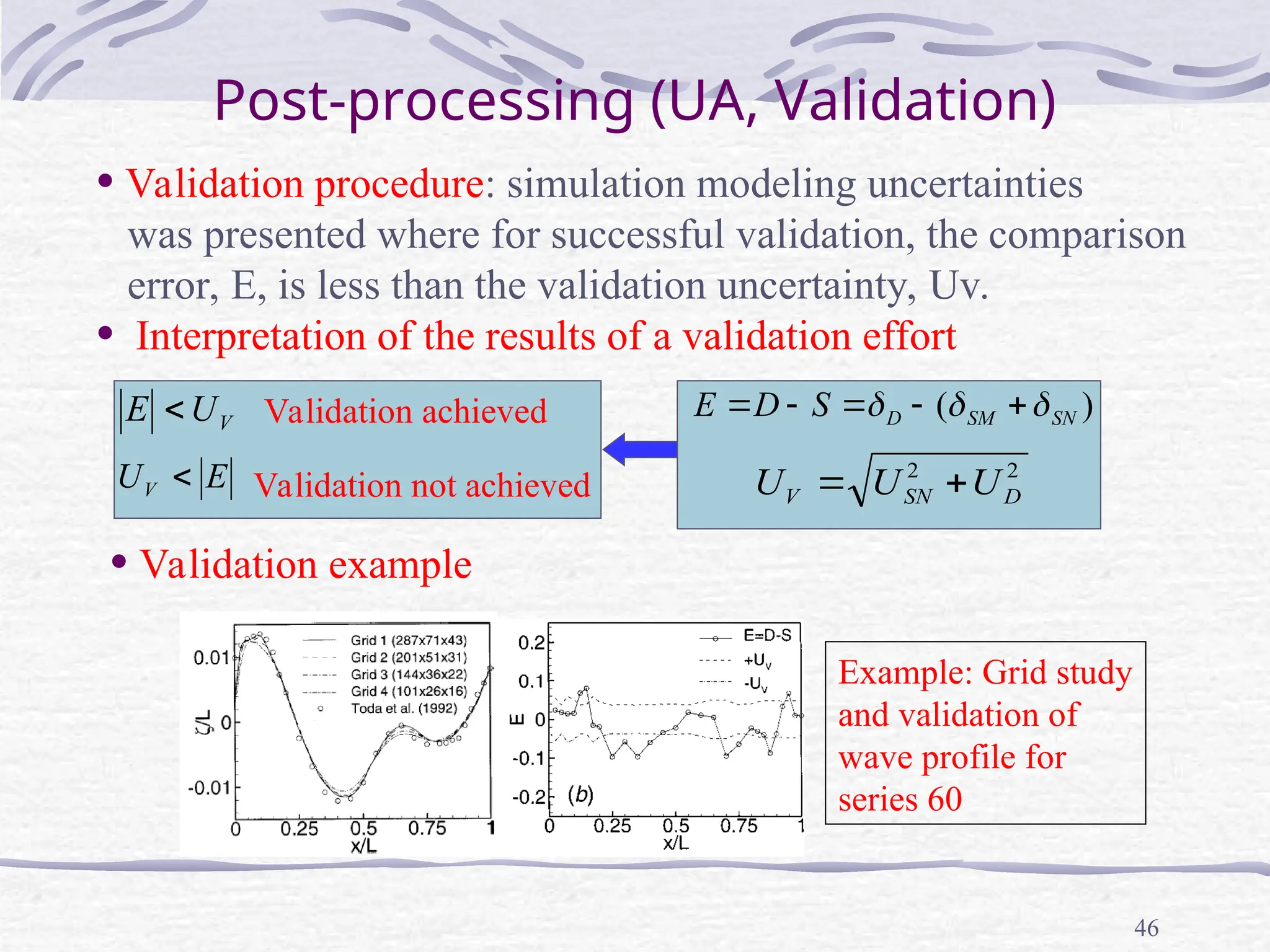
• Validation procedure: simulation modeling uncertainties
was presented where for successful validation, the comparison
error, E, is less than the validation uncertainty, Uv.
• Interpretation of the results of a validation effort
• Validation example
Example: Grid study
and validation of
wave profile for
series 60
2
2
D
SN
V U
U
U 

)
( SN
SM
D
S
D
E 

 





47. 47
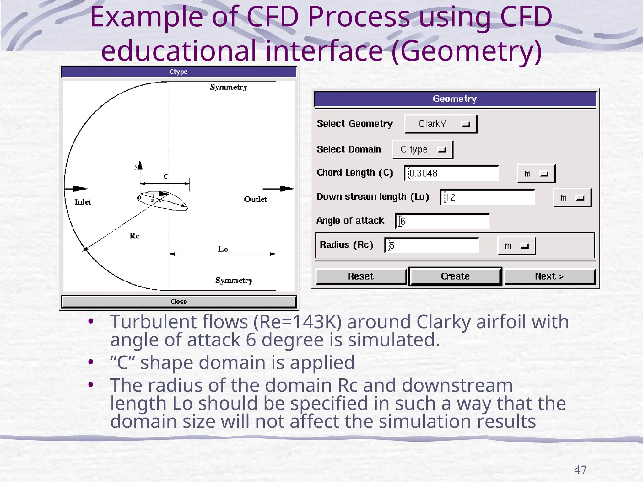
Example of CFD Process using CFD
educational interface (Geometry)
• Turbulent flows (Re=143K) around Clarky airfoil with
angle of attack 6 degree is simulated.
• “C” shape domain is applied
• The radius of the domain Rc and downstream
length Lo should be specified in such a way that the
domain size will not affect the simulation results

48. 48
Example of CFD Process (Physics)
No heat transfer

49. 49
Example of CFD Process (Mesh)
Grid need to be refined near the
foil surface to resolve the
boundary layer

50. 50
Example of CFD Process (Solve)
Residuals vs. iteration

51. 51
Example of CFD Process (Reports)

52. 52
processing)

53. 53
57:020 CFD Labs
• CFD Labs instructed by Shanti, Bhushan, Maysam Mousaviraad and Andrew Porter
• Use the educational interface — FlowLab 1.2.14
• Visit class website for more information
http://css.engineering.uiowa.edu/~fluids
CFD
Lab
CFD PreLab1 CFD Lab1 CFD PreLab2 CFD Lab 2
Dates Oct. 13, 15 Oct. 20, 22 Nov. 10, 12 Nov. 17, 19
Schedule