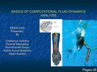
This document provides an overview of computational fluid dynamics (CFD) analysis. It discusses the basics of CFD, including its history, concepts, processes, governing equations, examples, applications, and sources of errors. The document was presented by Chaitanya Vudutha, Parimal Nilangekar, Ravindranath Gouni, and Satish Kumar Boppana to Albert Koether. It contains 28 pages covering topics such as laminar and turbulent flow, Newtonian and non-Newtonian fluids, discretization methods, the CFD process, and the Navier-Stokes equations. Applications of CFD include industries like aerospace, automotive, power generation, and meteorology.

1. BASICS OF COMPUTATIONAL FLUID DYNAMICS
ANALYSIS
MEEN 5330
Presented
By
Chaitanya Vudutha
Parimal Nilangekar
Ravindranath Gouni
Satish Kumar Boppana
Albert Koether
Pages-28

2. Overview
 Introduction
 History of CFD
 Basic concepts
 CFD Process
 Derivation of Navier-Stokes Duhem Equation
 Example Problem
 Applications
 Conclusion
 References

3. Introduction
What is CFD?
Prediction fluid flow with the complications of simultaneous
flow of heat, mass transfer, phase change, chemical reaction,
etc using computers
History of CFD
 Since 1940s analytical solution to most fluid dynamics problems was
available for idealized solutions. Methods for solution of ODEs or PDEs
were conceived only on paper due to absence of personal computer.
 Daimler Chrysler was the first company to use CFD in Automotive sector.
 Speedo was the first swimwear company to use CFD.
 There are number of companies and software's in CFD field in the world.
Some software's by American companies are FLUENT, TIDAL, C-MOLD,
GASP, FLOTRAN, SPLASH, Tetrex, ViGPLOT, VGRID, etc.

4. BASIC CONCEPTS
Fluid
Mechanics
Fluid Statics Fluid Dynamics
Laminar Turbulent
Newtonian Fluid Non-Newtonian Fluid
Ideal Fluids Viscous Fluids Rheology
Compressible Incompressible CFD Solutions for
Flow Flow specific Regimes
Components of Fluid Mechanics

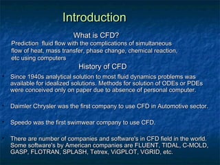
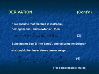
5. −6
volumes no smaller than say (1*10 m3)
Molecular Particles of Fluid
Basic fluid motion can be described as some combination of
1) Translation: [ motion of the center of mass ]
2) Dilatation: [ volume change ]
3) Rotation: [About one, two or 3 axes ].
4) Shear Strain

6. Compressible and Incompressible flow
A fluid flow is said to be compressible when
the pressure variation in the flow field is
large enough to cause substantial changes
in the density of fluid.
dqi 1 ~
µ
= f i − p,i + qi , jj
dt ρ ρ
Viscous and Inviscid Flow
In a viscous flow the fluid friction has
significant effects on the solution where
the viscous forces are more significant
than inertial forces
∂ ∂
( ρ u ) + ( ρ v) = 0
∂x ∂y

7. Steady and Unsteady Flow
Whether a problem is steady or unsteady depends on the frame of
reference
Laminar and Turbulent Flow
Newtonian Fluids and Non-Newtonian Fluids
In Newtonian Fluids such as water, ethanol, benzene
and air, the plot of shear stress versus shear rate at a
given temperature is a straight line

8. Initial or Boundary Conditions
 Initial condition involves knowing the state of pressure
(p) and initial velocity (u) at all points in the flow.
 Boundary conditions such as walls, inlets and outlets
largely specify what the solution will be.

9. Discretization Methods
 Finite volume • Where Q - vector of conserved variables
method
• F - vector of fluxes
∂ • V - cell volume
∂t ∫∫∫ Qdv + ∫∫ FdA = 0
• A –Cell surface area
 Finite Element
method Ri=Equation residual at an element vertex
Q- Conservation equation expressed on element
basis
Ri = ∫∫∫Wi Qdv e Wi= Weight Factor

10.  Finite difference method
∂Q ∂F ∂G ∂H
+ + + =0
∂t ∂x ∂y ∂z Q – Vector of conserved variables
F,G,H – Fluxes in the x ,y, z directions
Boundary element method
The boundary occupied by the fluid is divided into
surface mesh

11. CFD PROCESS
 Geometry of problem
is defined .
 Volume occupied by
fluid is divided into
discrete cells.

12. CFD PROCESS cont..
Physical modeling is defined.
Boundary conditions are defined
which involves specifying of fluid
behavior and properties at the
boundaries.
Equations are solved iteratively
as steady state or transient state.
Analysis and visualization of
resulting solution. post processing

13. DERIVATION OF NAVIER-STOKES-DUHEM
EQUATION
The Navier-Stokes equations are the fundamental partial
differentials equations that describe the flow of incompressible
fluids.
Two of the alternative forms of equations of motion, using
the Eulerian description, were given as Equation (1) and
Equation (2) respectively:
∂( ρqi )
+ ( ρq i q j ) , j = ρf i + σ ji , j (1)
∂t
dq i ∂q i 1
= + q j qi , j = f i + σ ji , j . (2)
dt ∂t ρ

14. DERIVATION (Cont’d)
If we assume that the fluid is isotropic ,
homogeneous , and Newtonian, then :
~ ~
σ ij = −( p − λ ∈kk )δ ij + 2 µ ∈ij . (3)
Substituting Equ(3) into Equ(2), and utilizing the Eulerian
relationship for linear stress tensor we get :
dqi 1 ~ ~
µ +λ ~
µ
= f i − p ,i + q j , ji + qi , jj , (4)
dt ρ ρ ρ
( for compressible fluids )

15. DERIVATION
(Cont’d)
For incompressible fluid flow the Navier-Stokes-
Duhem equation is:
dqi 1 ~
µ
= f i − p,i + qi , jj
dt ρ ρ
If the fluid medium is a monatomic ideal gas, then :
~ 2 ~
λ =− µ
3

16. DERIVATION (Cont’d)
Navier stokes equation for compressible flow of
monatomic ideal gas is :
dqi 1 ~
1µ ~
µ
= f i − p ,i + q j , ji + qi , jj ,
dt ρ 3ρ ρ

17. EXAMPLE PROBLEM
Neglecting the gravity field, describe the steady two-
dimensional flow of an isotropic , homogeneous,
Newtonian fluid due to a constant pressure gradient
between two infinite, flat, parallel, plates. State the
necessary assumptions. Assume that the fluid has a
uniform density.

18. SOLUTION (Cont’d)
The Navier – stokes equations for incompressible flow is:
dqi 1 ~
µ
+ q j qi , j = f i − p,i + qi , jj
dt ρ ρ
Since the flow is steady and the body forces are
neglected, the Navier-stokes equation becomes:
1 ~
µ
q j qi , j = − p,i + qi , jj
ρ ρ

19. SOLUTION (Cont’d)
The no slip boundary conditions for viscous flow are:
qi = 0 at y2 = ±a
Using the boundary conditions ( q2= 0 at y2=+/- a )
Thus, the first Navier-stokes equations becomes
d 2 q1 dp
µ 2
=
dy 2 dy1

20. SOLUTION (Cont’d)
Integrating twice, we obtain
q1 =
1 dp 2
2 µ dy1
(
y2 − a 2 )
The results, assumptions and boundary conditions of this
problem in terms of, mathematical symbols are as follows:
ρ = Constant ∂ )
( =0 ∂( )
fi = 0 =0
∂ t ∂y 3
q1 =
1 dp 2
2µ dy1
( y2 − a 2 )

21. HOMEWORK PROBLEM
 Using the Navier-Stokes equations investigate the flow (q i) between
two stationary, infinite, parallel plates a distance h apart. Assuming
that you have laminar flow of a constant-density, Newtonian fluid
and the pressure gradient is constant (partial derivative of P with
respect to 1).

22. Types of Errors and Problems
Types of Errors:
 Modeling Error.
 Discretization Error.
 Convergence Error.
Reasons due to which Errors occur:
 Stability.
 Consistency.
 Conservedness and Boundedness.

23. Applications of CFD
1. Industrial Applications:
CFD is used in wide variety of disciplines and industries,
including aerospace, automotive, power generation, chemical
manufacturing, polymer processing, petroleum exploration,
pulp and paper operation, medical research, meteorology, and
astrophysics.
Example: Analysis of Airplane
CFD allows one to simulate the reactor
without making any assumptions about the
macroscopic flow pattern and thus to
design the vessel properly the first time.

24. Application (Contd..)
2. Two Dimensional Transfer Chute Analyses Using a
Continuum Method:
Fluent is used in chute designing tasks like predicting flow shape,
stream velocity, wear index and location of flow recirculation
zones.
3. Bio-Medical Engineering:
The following figure shows pressure
contours and a cutaway view that
reveals velocity vectors in a blood
pump that assumes the role of heart
in open-heart surgery.
Pressure Contours in Blood Pump

25. Application (Contd..)
4. Blast Interaction with a Generic Ship Hull
The figure shows the
interaction of an explosion
with a generic ship hull.
The structure was modeled
with quadrilateral shell
elements and the fluid as a
mixture of high explosives
and air. The structural
elements were assumed to
fail once the average strain
Results in a cut plane for the interaction of an
in an element exceeded 60 explosion with a generic ship hull: (a) Surface
percent at 20msec (b) Pressure at 20msec (c)
Surface at 50msec and (d) Pressure at
50msec

26. Application (Contd..)
5. Automotive Applications:
Streamlines in a vehicle without (left) and with rear center and B-pillar ventilation (right)
In above figure, influence of the rear center and B-pillar ventilation on the
rear passenger comfort is assessed. The streamlines marking the rear
center and B-pillar ventilation jets are colored in red. With the rear center
and B-pillar ventilation, the rear passengers are passed by more cool air. In
the system without rear center and B-pillar ventilation, the upper part of the
body, in particular chest and belly is too warm.

27. Conclusion
 Nearer the conditions of the experiment to those which concern
the user, more closely the predictions agree with those data, the
greater is the reliance which can be prudently placed on the
predictions.
 CFD iterative Methods like Jacobi and Gauss-Seidel Method are
used because the cost of direct methods is too high and
discretization error is larger than the accuracy of the computer
arithmetic.
 Many software’s offer the possibility of solving fully nonlinear
coupled equations in a production environment.
 In the future we can have a multidisciplinary, database linked
framework accessed from anywhere on demand simulations with
unprecedented detail and realism carried out in fast succession so
that designers and engineers anywhere in the world can discuss
and analyze new ideas and first principles driven virtual reality

28. References
1. Hoffmann, Klaus A, and Chiang, Steve.T “Computational fluid dynamics
for engineer’s” vol. I and vol. II
2. Rajesh Bhaskaran, Lance Collins “Introduction to CFD Basics”
3. http://www.cham.co.uk/website/new/cfdintro.htm accessed on 11/10/06.
4. Adapted from notes by: Tao Xing and Fred Stern, The University of Iowa.
5. http://www.cfd-online.com/Wiki/Historical_perspective accessed on
11/12/06.
6. Frederick and Chang,T.S.,”Continuum Mechanics”
7. http://navier-stokes-equations.search.ipupdate.com/
8. http://en.wikipedia.org/wiki/Computational_fluid_dynamics#Discretization_
method s, ”Discretization Methods”
9. McIlvenna P and Mossad R “Two Dimensional Transfer Chute Analysis
Using a Continuum Method”, Third International Conference on CFD in
the Minerals and Process Industries, Dec 2003.
10. Subramanian R.S. “Non-Newtonian Flows”.
11. Lohner R., Cebral J., Yand C., “Large Scale Fluid Structure Interaction
Simulations, IEEE June 2004”.
12. http://www.cd-
adapco.com/press_room/dynamics/23/behr.html,“Predicting Passenger
Comfort
13. http://www.adl.gatech.edu/classes/lowspdaero/lospd2/lospd2.html,
“Types of Fluid Motion”

29. Thank You
Questions are Welcome