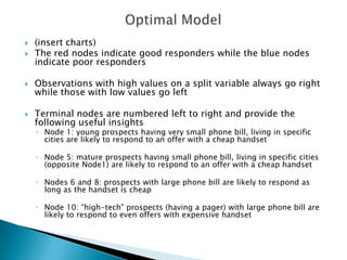
Downloaded 54 times


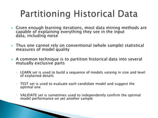
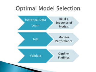


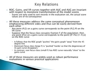
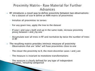
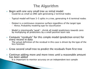
![ The following approach will take full advantage of the set of
continuous scores produced by Rank or Probability models
Pick one of the two target classes as the class in focus
Sort a database by predicted score in descending order
Choose a set of different score values
◦ Could be ALL of the unique scores produced by the model
◦ More often a set of scores obtained by binning sorted records into equal
size bins
For any fixed value of the score we can now compute:
◦ Sensitivity (a.k.a True Positive): Percent of the class in focus with the
predicted scores above the threshold
◦ Specificity (a.k.a False Positive): Percent of the opposite class with the
predicted scores below the threshold
We then display the results as a plot of [sensitivity] versus [1-specificity]
The resulting curve is known as the ROC Curve](https://image.slidesharecdn.com/informspresentationnewppt-120210180702-phpapp02/85/Informs-presentation-new-ppt-21-320.jpg)


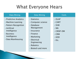
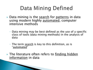
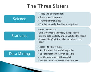
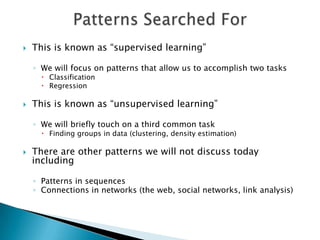
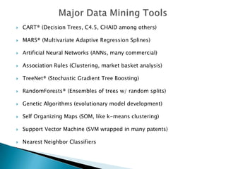
This document provides an overview of data mining concepts and techniques. It discusses topics such as predictive analytics, machine learning, pattern recognition, and artificial intelligence as they relate to data mining. It also covers specific data mining algorithms like decision trees, neural networks, and association rules. The document discusses supervised and unsupervised learning approaches and explains model evaluation techniques like accuracy, ROC curves, gains/lift curves, and cross-entropy. It emphasizes the importance of evaluating models on test data and monitoring performance over time as patterns change.