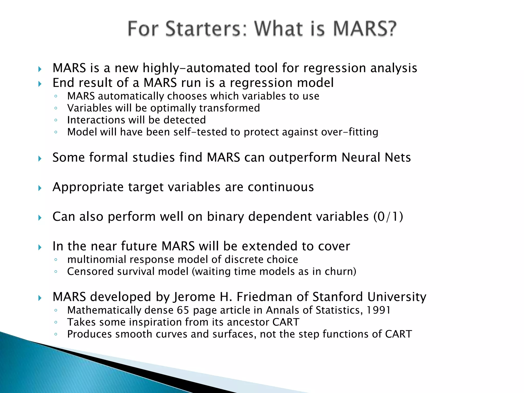
TreeNet Tree Ensembles and CART Decision Trees: A Winning Combination
MARS Regression Analysis Tool for Automated Modeling
1.
2. Salford Systems
8880 Rio San Diego Drive, Suite 1045
San Diego, CA. 92108
619.543.8880 tel
619.543.8888 fax
www.salford-systems.com
dstein@salford-systems.com
3. MARS is a new highly-automated tool for regression analysis
End result of a MARS run is a regression model
◦ MARS automatically chooses which variables to use
◦ Variables will be optimally transformed
◦ Interactions will be detected
◦ Model will have been self-tested to protect against over-fitting
Some formal studies find MARS can outperform Neural Nets
Appropriate target variables are continuous
Can also perform well on binary dependent variables (0/1)
In the near future MARS will be extended to cover
◦ multinomial response model of discrete choice
◦ Censored survival model (waiting time models as in churn)
MARS developed by Jerome H. Friedman of Stanford University
◦ Mathematically dense 65 page article in Annals of Statistics, 1991
◦ Takes some inspiration from its ancestor CART
◦ Produces smooth curves and surfaces, not the step functions of CART
4. Introduction to the core concepts of MARS
◦ Adaptive modeling
◦ Smooths, splines and knots
◦ Basis functions
◦ GCV: generalized cross validation and model selection
◦ MARS handling of categorical variables and missing values
Guide to reading the classic MARS output
◦ MARS ANOVA Table
◦ Variable Importance
◦ MARS coefficients
◦ MARS diagnostic
Advice on using MARS software in practice
◦ Problems MARS is best suited for
◦ How to tweak core control parameters
◦ Incorporating MARS into your analysis process
◦ Brief introduction to the latest MARS software
5. Harrison, D. and D. Rubinfeld. Hedonic Housing Prices and Demand For
Clean Air. Journal of Environmental Economics and Management, v5, 81-
102, 1978
◦ 506 census tracts in City of Boston for the year 1970
◦ Goal: study relationship between quality of life variables and property values
◦ MV median value of owner-occupied homes in tract („000s)
◦ CRIM per capita crime rates
◦ NOX concentration of nitrogen oxides (pphm)
◦ AGE percent built before 1940
◦ DIS weighted distance to centers of employment
◦ RM average number of rooms per house
◦ LSTAT percent neighborhood „lower SES‟
◦ RAD accessibility to radial highways
◦ ZN percent land zoned for lots
◦ CHAS borders Charles River (0/1)
◦ INDUS percent non-retail business
◦ TAX tax rate
◦ PT pupil teacher ratio
6. Data set also discussed in Belsley, Kuh, and
Welsch, 1980, Regression Diagnostics, Wiley.
Breiman, Friedman, Olshen, and
Stone, 1984, Classification and Regression
Trees, Wadsworth
(insert table)
8. Clearly some non-normal distributions and
non-linear relationships
(insert graph)
9. Modeler‟s job is to find a way to accurately predict y given some
variables x
Can be thought of as approximating the generic function y=f(x)+ noise
Problem is: modeler doesn‟t know enough to do this as well as we would
like
First: modeler does not know which x variables to use
◦ Might know some of them, but rarely knows all
Second: modeler does not know how variables combine to generate y i.e.
does not know the mathematical form for f(X)
Even if we did know which variables were needed
◦ Do not know the functional form to use for any individual variable
Log, square root, power, inverse, S-shaped
◦ Do not know what interactions might be needed and what degree of interaction
10. Parametric Statistical modeling is a process of trial and error
◦ Specify a plausible model (based on what we already think we know)
◦ Specify plausible competing models
◦ Diagnose Residuals
◦ Test natural hypotheses (e.g. do specific demographics affect behavior?)
◦ Assess performance (goodness of fit, lift, Lorenz curve)
Compare to performance of other models on this type of problem
◦ Revise model in light of tests and diagnoses
◦ Stop when time runs out or improvements in model become negligible
Never enough time for modeling (always comes last)
◦ Particularly if database is large and contains many fields
◦ Large databases (many records) invite exploration of more complex models
Quality of result highly dependent on skill of modeler
◦ Easy to overlook an important effect
◦ Also easy to be fooled by data anomalies (multivariate outliers, data errors)
◦ We have encountered many statistician-developed models with important errors
11. Modern tools learn far more about the best model from data itself
◦ Modern tools started coming online in the 1980‟s and 1990‟s (see references)
◦ All compute intensive: would never have been invented in the pre-computer era
◦ Frequently involve intelligent algorithms AND brute force searches
Some methods let data dictate functional form id given the variables
◦ Modeler selects variables and specifies most of the model
◦ Method determines functional form for a variable (e.g. GAM, Generalized Additive
Model)
Other methods are fully automatic for both variable selection and
functional form (e.g. CART® and MARS™)
Important not to be overly driven:
◦ A prior knowledge can be very valuable
Can help shape model when several alternatives are all consistent with data
Can help detect errors (e.g. price increases normally reduce Q demanded)
Proper constraints can yield better models
◦ Automatic methods can yield problematic models
No risk yet that analysis's are in danger of being displaced by software
12. Intended use of the final model will influence how we develop it
Predictive accuracy
◦ If this is the sole criterion by which model is to be assessed then its complexity and
comprehensibility is irrelevant
However, difficult to assess a model that we cannot understand
◦ Can use modern tools such as boosted decision trees or neural nets
These methods do not yield models that are easy to understand
◦ Boosted decision trees combine perhaps 800 smallish trees, each tree uses a different
set of weights on the training data and results averaged
Understanding the data generation process
◦ Want a representation of the causal process itself
◦ Also want a model that can be understood
Desire to tell a story
Use insights to make decisions
◦ Can use single decision trees or regression-like models
Both yield results that can assist understanding
We assume understanding is one of the modeler‟s goals for this tutorial
13. Global parametric modeling such as logistic regression
◦ Rapid computation
◦ Accurate only if specified model is reasonable approximation to true function
◦ Typical parametric models have limited flexibility
Parametric models usually give best performance when simple
Extensions to model specification such as polynomials in predictors can disastrously
mistrack
Means that good approximation may be impossible to obtain if reality is sufficiently
complex
◦ Can work well even with small data sets (only need two points to define a line!)
With smaller data sets no choice but to go parametric
◦ All data points influence virtually all aspects of the model
◦ Best example is simple linear regression: all points help to locate line
◦ Strength and weakness:
Strengths include efficiency in data use
Can be very accurate when developed by expert modelers
Weaknesses include vulnerability to outliers and missing subtleties
14. Linear regression of MV on percent lower SES
◦ All data influence line; high MV values at low
LSTAT pulls regression line up
◦ (insert graph)
15. Fully nonparametric modeling develops model locally rather than
globally
◦ One extreme: simply reproduce the data (not a useful model)
◦ Need some kind of simplification or summary
◦ Smoothing is an example of such simplification
Identify a small region of the data
◦ Example: low values of X1, or low values of X1, X2 and X3
Summarize how the target variable y behaves in this region
◦ Single value for entire region such as average value or median
◦ Or fit curve, surface, or regression just for this region
Develop a separate summary in each region of the predictor space
Analyst might wish to require some cross region smoothness
◦ Neighboring regions have to have function join up (no jumps as in CART)
◦ Can require that first derivative continuous (so even smoother)
◦ Some smooths require continuous 2nd derivative (limit of what eye can usually see)
16. Median smooth: for each value of LSTAT
using a 10% of data window to determine
smoothed value for predicted MV
(Insert graph)
17. The kernel density estimator: insert equation
K() is a weighting function known as a kernel function
◦ K() integrates to 1
◦ Typically a bell-shaped curve like the normal, so weight declines with
distance from center of interval:
◦ There is a separate K() for EVERY data value Xj
B is a bandwidth, size of a window about Xj
◦ For some kernels data outside of window have a weight of zero
◦ Within data window K() could be a constant
◦ The smaller the window the more local the estimator
18. Smooths available in several statistical graphics packages
Common smooths include
◦ Running mean
◦ Running median
◦ Distance Weighted Least Squares (DWLS)
Fit new regression at each value of X, downweight points by distance from
current value of X
◦ LOWESS and LOESS
These are locally weighted regression smooths
Latter also downweights outliers from local regressions
Almost all smooths require choice of a tuning parameter
◦ Typically a “window” size: how large a fraction of the data to use when
evaluating smooth for any value of X
◦ The larger the window the less local and the more smooth the result
Next two slides demonstrate two extremes of smoothing
19. Actually uses 50% on either side of current X, still
over smoothed
(insert graph)
20. Super flexible segments using 5% intervals of
the data
(insert graph)
21. Goal is to predict y as a function of x
To estimate the expected value of y for a specific set of X‟s, find data
records with that specific set of x‟s
If too few (or no) data points with that specific set of x‟s then make do
with data points that are “close”
◦ Possibly use data points that are not quite so close but down-weight them
◦ Bringing points from further away will contribute to bias
How to define a local neighborhood (what is close?)
◦ Size of neighborhood can be selected by user
◦ Best neighborhood size determined via experimentation, cross-validation
How to down-weight observations far away from a specific combination
of x‟s
◦ Large number of weighting functions (kernels) available
◦ Many are bell-shaped
◦ Specific kernel used less important than bandwidth
22. The more global a model, the more likely it is to be biased for at
least some regions of x
◦ Bias: expected result is incorrect (systematically too high for some values
of X and systematically too low for other values of X)
◦ But since it makes use of all the data it should have low variance
i.e stable results from sample to sample
The more local a portion of a model, the higher the variance is
likely to be (because the amount of relevant data is small)
◦ But being local it is faithful to the data and will have low bias
Simple (global) models tend to be stable (and biased)
Classic example from insurance risk assessment
◦ Estimate risk that restaurant will burn down in small town (few
observations)
◦ “borrow” data from other towns (less relevant but gives you more data)
◦ Can look for an optimal balance of bias and variance
One popular way to balance bias and variance is to minimize MSE
The best way to balance will depend on precise goals of model
23. Squared Error Loss function typical for any approximation
to the non-linear function f(X)
(insert equation)
Variance here measures how different the model
predictions would be from training sample to training
sample
◦ Just how stable can we expect our results to be
Bias measures the tendency of the model to systematically
mistrack
MSE is sensitive to outliers so other criteria can be more
robust
24. Most research in fully nonparametric models focuses on
functions with 1,2, or 3 predictors!
David W. Scott. Multivariate Density Estimation. Wiley, 1992.
◦ Suggests practical limit of 5 dimensions
◦ More recent work may have pushed this up to 8 dimensions
Attempt to use these ideas directly in the context of most market
research or data mining contexts is hopeless
Suppose we decide to look at two regions only for each variable
in a database, values below average and values above average
With 2 predictors we will have 4 regions to investigate:
◦ Low/low,low/high,high/low, and high/high
25. With 3 variables will have 8 regions, with 4 variables, 16 regions
Now consider 35 predictor variables
Even with only 2 intervals per variable this generates 2^35 regions (34
billion regions) most of which would be empty
◦ 2^16= 65,536
◦ 2^32= 4.3 billion (gig)
Many market research data sets have less than a million records
Clearly infeasible to approximate the function y=f(x) by summarizing y
in each distinct region of x
For most variables two regions will not be enough to track the specifics
of the function
◦ If the relationship of y to some x‟s is different in 3 or 4 regions of each predictor then
the number of regions needing to be examined is even larger than 2^35 with only 35
variables
Number of regions needed cannot be determined a priori
◦ So a serious mistake to specify too few regions in advance
26. Need a solution that can accomplish the following
◦ Judicious selection of which regions to look at and their boundaries
◦ Judicious determination of how many intervals are needed for each
variable
e.g. if function is very “squiggly” in a certain region we will want many
intervals; if the function is a straight line we only need one interval
◦ A successful method will need to be ADAPTIVE to the characteristics of the
data
Solution will typically ignore a good number of variables (variable
selection)
Solution will have us taking into account only a few variables at a
time (again reducing the number of regions)
◦ Thus even if method selects 30 variables for model it will not look at all 30
simultaneously
◦ Consider decision tree; at a single node only ancestor splits are being
considered so a depth of six only six variables are being used to define
node
27. Two major types of splines:
◦ Interpolating- spline passes through ever data point (curve drawing)
◦ Smoothing- relevant for statistics, curve needs to be “close” to data
Start by placing a uniform grid on the predictors
◦ Choose some reasonable number of knots
Fit a separate cubic regression within each region (cubic spline)
◦ Most common form of spline
◦ Popular with physicists and engineers for whom cts 2nd derivatives
required
Appears to require many coefficients to be estimated (4 per
region)
Normally constraints placed on cubics
◦ Curve segments must join (overall curve is continuous)
◦ Continuous 1st derivative at knots (higher degree of smoothness)
◦ Continuous 2nd derivative at knots (highest degree of smoothness)
Constraints reduce the number of free parameters dramatically
28. Impose a grid with evenly spaced intervals on the x-axis
L ----+---+---+---+---+---+---+---U
◦ L is lower boundary, U is upper boundary
On each segment fit the function
◦ (insert equation)
Apparently four free parameters per cubic function
The cubic polynomials must join smoothly with continuous 2nd
derivatives
Typically there are also some end point or boundary conditions
◦ e.g. 2nd derivative goes to zero
Very simple to implement; but a linear regression on the
appropriate regressors
This approach to splines is mentioned for historical reasons only
29. Piece-Wise Linear Regression
◦ Simplest version of splines well know for some time:
Instead of a single straight line to fit to data
allow regression to bend
Example:
◦ MARS spline with 3 knots superimposed on the actual
data
◦ (insert graph)
30. Knot marks the end of one region of data and the
beginning of another
Knot is where the behavior of the function changes
◦ Model could well be global between knots (e.g. linear regression)
◦ Model becomes local because it is different in each region
In a classical spline the knot positions are predetermined
and are often evenly spaced
In MARS, knots are determined by search procedure
Only as many knots as needed end up in the MARS model
If a straight line is a good fit there will be no interior knots
◦ In MARS there is always at least one boundary knot
◦ Corresponds to the smallest observed value of the predictor
31. With only one predictor and one knot to select, placement is
straightforward:
◦ Test every possible knot location
◦ Choose model with best fit (smallest SSE)
◦ Perhaps constrain by requiring a minimum amount of data in each interval
Prevents the one interior knot being placed too close to a boundary
Potential knot locations:
◦ Cannot directly consider all possible values on the real line
◦ Often only actual data values are examined
◦ Advantageous to also allow points between actual data values (say mid-
point)
Better fit might be obtained if change in slope allowed at a mid-point rather
than at an actual data value
It is actually possible to explicitly solve for the best knot lying between two
actual data values
Piece-wise linear splines can reasonably approximate quite
complex functions
32. True knot occurs at x=150
No data available between x=100 and x=200
(insert graph)
33. Finding the one best knot in a simple regression is a
straightforward search problem:
◦ Try a large number of potential knots and choose one with best R-squared
◦ Computation can be implemented efficiently using update algorithms;
entire regression does not have to be rerun for every possible knot (just
update X‟X matrices)
Finding the best pair of knots will require far more computation
◦ Brute force search possible- examine all possible pairs
◦ Requires order of N^2 tests
◦ If we needed 3 knots order of N^3 tests would be required
◦ Finding best single knot and then finding best to add next may not find
the best pair of knots
◦ Simple forward stepwise search could easily get the wrong result
Finding best set of knots when the number of knots needed is
unknown is an even more challenging problem
34. True function (in graph on left) has two knots
at x=30 and x=60
Observed data at right contains random error
Best single knot will be at x=45 and MARS
finds this first
(insert graphs)
35. Start with one knot- then steadily increase
number of allowed knots
(insert graph)
36. Solution for finding the location and number of needed knots
can be solved in a stepwise fashion
Need a forward/backward procedure as used in CART
First develop a model that is clearly overfit with too many knots
◦ e.g. in a stepwise search find 10 or 15 knots
Follow by removing knots that contribute least to fit
Using appropriate statistical criterion remove all knots that add
sufficiently little to model quality
◦ Although not obvious what this statistical criterion will be
Resulting model will have approximately correct knot locations
◦ Forward knot selection will include many incorrect knot locations
◦ Erroneous knot locations should eventually be deleted from model
But this is not guaranteed
◦ Strictly speaking there may not be a true set of knot locations as the true
function may be smooth
37. When seven knots are allowed MARS tries:
◦ 26.774, 29.172, 45.522, 47.902, 50.425, 58.600, 61.74
7
Recall that true knots are at 30 and 60
MARS discards some of the knots, but keeps a
couple too many
◦ 29.172, 45.522, 47.902, 61.747
MARS persists in tracking a wobble in the top of
the function
38. Thinking in terms of knot selection works very well to illustrate
splines in one dimension
Thinking in terms of knot locations is unwieldy for working with
a large number of variables simultaneously
◦ Need a concise notation and programming expressions that are easy to
manipulate
◦ Not clear how to construct or represent interactions using knot locations
Basis: A set of functions used to capture the information
contained in one or more variables
◦ A re-expression of the variables
◦ A complete set of principal components would be a familiar example
◦ A weighted sum of basis functions will be used to approximate the
function of interest
MARS creates sets of basis functions to decompose the
information in each variable individually
39. The hockey stick basis function is the core building block
of the MARS model
◦ Can be applied to a single variable multiple times
Hockey stick function:
◦ Max (0,X-c)
◦ Max (0,c-X)
◦ Maps variable X to new variable X*
◦ X* is set 0 for all values of X up to some threshold value c
◦ X* is equal to X (essentially) for all values of X greater than c
◦ Actually X* is equal to the amount by which X exceeds threshold c
40. X ranges from 0 to 100
8 basis functions displayed
(c=10,20,30,…80)
(insert graph)
41. Each function is graphed with same dimensions
BF10 is offset from original value by 10
BF80 is zero for most of its range
Such basis functions can be constructed for any value of c
MARS considers constructing one for EVERY possible data
value
43. Define a basis function BF1 on the variable INDUS:
◦ BF1= max (0,INDUS-4)
Use this function instead of INDUS in a regression
◦ Y= constant + β*BF1+ error
This fits a model in which the effort of INDUS on the dependent
variable is 0 for all values below 4 and β for values above 4
Suppose we added a second basis function BF2 to the model:
◦ BF2= max (0,INDUS-8)
Then our regression function would be
◦ Y=constant+ β*BF1 + β*BF2 +error
This fits a model in which the effort of INDUS on y is
◦ 0 for UNDUS<=4
◦ β for 4<=INDUS<=8
◦ β1 + β2 for INDUS >8
44. (insert data)
Note that max value of the BFs is just shifted
max of original
Mean is not simply shifted as max() is a non-
linear function
Alternative notation for basis function:
◦ (X-knot)
Has same meaning as MAX(0,X- knot)
46. MV= 30.290-2.439*(INDUS-4) +2.215*(INDUS-8)
Slope starts at 0 and then becomes -2.439 after INDUS=4
Slope on third portion (after INDUS=8) is (-2.439+2.215)= -
0.224
(insert graph)
47. A standard basis function (X-knot) does not
provide for a non-zero sloe for values below the
knot
To handle this MARS uses a “mirror image” basis
function
Mirror image basis function on left, standard on
right
(insert graph)
48. The mirror image hockey stick function looks at the interval of a
variable X which lies below the threshold c
Consider BF=max(0,20,-X)
This is downward sloping at 45 degrees; is has value 20 when X
is 0 and declines until it hits 0 at X=20 and remains 0 for all
other X
It is just a mathematical convenience: with a negative coefficient
it yields any needed slope for the X interval 0 to 20
Left panel is mirror image BF, right panel is basis function *-1
(insert graph)
49. We now have the following basis functions in INDUS
(insert equation)
All 3 line segments have negative slopes even
though 2 coefficients above>0
(insert graph)
50. By their very nature any hockey stick function defines a knot
where a regression can change slope
Running a regression on hockey stick functions is equivalent to
specifying a piecewise linear regression
So the problem of locating knots is now translated into the
problem of defining basis functions
Basis functions are much more convenient to work with
mathematically
◦ For example you can interact a basis function from one variable with a
basis function from another variable
◦ The programming code to define a basis function is straightforward
Set of potential basis functions: can create one for every possible
data value of every variable
51. Actually MARS creates basis functions in pairs
◦ Thus twice as many basis functions possible as there are distinct
data values
◦ Reminiscent of CART (left and right sides of split)
◦ Mirror image is needed to ultimately find right model
◦ Not all linearly independent but increases flexibility of model
For a given set of knots only one mirror image basis
function will be linearly independent of the standard basis
functions
◦ Further, it won‟t matter which mirror image basis function is
added as they will all yield the same model
However, using the mirror image INSTEAD of the standard
basis function at any knot will change the model
52. MARS generates basis functions by searching in a stepwise manner
Starts with just a constant in the model
Searches for variable-knot combination that improves model the most
(or worsens model the least)
◦ Improvement measured in part by change in MSE
◦ Adding a basis function will always reduce MSE
◦ Reduction is penalized by the degrees of freedom used in knot
◦ Degrees of freedom and penalty addressed later
Search is for a PAIR of hockey stick basis functions (primary and mirror
image)
◦ Even though only one might be linearly independent of other terms
Search is then repeated for best variable to add given basis functions
already in the model
Process is theoretically continued until every possible basis function has
been added to model
53. MARS technology is similar to CART‟s
◦ Grow a deliberately overfit model and then prune back
◦ Core notion is that good model cannot be built fro a forward stepping plus
stopping rule
◦ Must overfit generously and then remove unneeded basis functions
Model still needs to be limited
◦ With 400 variables and 10,000 records have potentially 400*10,000=4
million knots just for main effects
◦ Even if most variables have a limited number of distinct values (dummies
only allow one knot, age may only have 50 distinct values) total possible
will be large
In practice user specifies an upper limit for number of knots to
be generated in forward stage
◦ Limit should be large enough to ensure that true model can be captured
◦ At minimum twice as many basis functions as needed in optimal model
◦ Will have to be set by trial and error
◦ The larger the number the longer the run will take!
54. MARS categorical variable handling is almost exactly like CART‟s
The set of all levels of the predictor is partitioned into two
e.g. for States in the US the dummy might be 1 for
{AZ, CA, WA, OR, NV} and 0 for all other states
◦ A new dummy variable is created to represent this partition
◦ This is the categorical version of a basis function
As many basis functions of this type as needed may be created
by MARS
◦ The dummied need not be orthogonal
◦ e.g. the second State dummy (basis function could be 1 for {MA, NY, AZ}
which overlaps with the dummy defined above (AZ is in both)
◦ Theoretically, you could not get one dummy for each level of the
categorical predictor, but in practice levels are almost always grouped
together
Unlike continuous predictors, categorical predictors generate
only ONE basis function at a time since the mirror image would
just be the flipped dummy
55. For any categorical predictor the value of the variable can be
thought of as the level of the predictor which is “on”
◦ And of course all other levels are “off”
Can be represented as a string consisting of a single “1” in a
sequence of “0‟s”
◦ 000100 means that the 4th level of a six-level categorical is “on”
MARS uses this notation to represent splines in a categorical
variable
◦ 010100 represents a dummy variable that is coded “1” if the categorical
predictor in question has value 2 or 4
◦ 101011 is also created implicitly- the complementary spline
Technically, MARS might create the equivalent of a dummy for
each level separately (100000,010000,00100,00010,000001)
In practice this almost never happens
◦ Instead MARS combines levels that are similar in the context
56. Where RAD is declared categorical, MARS reports in
classic output:
(insert table)
Basis functions found
(insert functions)
Categorical predictors will not be graphed
57. Constant, always entered into model first, becomes basis
function 0
Two basis functions for INDUS with not at 8.140 entered
next
Then dummies for RAD=(1,4,6,24) and its complement
entered next
Then dummies for RAD=(4,6,8) and its complement
entered next
Continues until maximum number of basis functions
allowed in reach
(insert table)
58. Stated preference choice experiment conducted in Europe
early 1990s; focused on sample of persons interested in
cell phones
Primary attributes:
◦ Usage charges (presented as typical per month if usage was 100
minutes)
◦ Cost of equipment
Demographics and other Respondent Information
◦ Sex, Income, Age
◦ Region of residence
◦ Occupation, Type of Job, Self-employed, etc.
◦ Length of commute
◦ Ever had a cell phone, Have cell phone now
◦ Typical use for cell phone (business, personal)
◦ PC, Home, Fax, portable home phone, etc.
◦ Average land line phone bill
59. Original model: main effects, additive
◦ Model included two prices and dummies for levels of all
categorical predictors
◦ Log-likelihood- 133964 on 31 degrees of freedom
N~3,000
MARS model 1: main effects but with optimal
transform of prices
◦ Results adds one basis function to original model to
capture spline
◦ Log likelihood -133801 on 32 degrees of freedom (Chi-
square=126 on 1 df)
60. Best way to grasp MARS model is to review the
basis function code
Necessary supplement to the graphs produced
We review entire set below
(insert table)
61. First we have a mirror image pair for land line phone bill
◦ (insert functions)
No other basis functions in this variable, so we have a single knot
Next we have only the UPPER basis function in monthly cost and not
the mirror image basis function
◦ BF3= max(0, monprice-5,000)
◦ Means there is a zero slope until the knot and then a downward slope
◦ We read the slope from the coefficient reported
◦ With no basis function corresponding to monthly price below 5, slope for
this lower portion of prices is zero
The next basis function wants to keep the variable linear (no knot)
◦ Knot is placed at the minimum observed data value for the variable
◦ Technically a knot, but practically not a knot
◦ (Insert function)
There are a couple other similar basis functions in the model
62. The next basis functions represent a type we have not seen
before
◦ (insert function)
The first is an indicator for non-missing income data
The second is an indicator for missing income data
Such basis functions can appear in the final model either by
themselves or interacted with other variables
In this example, BF10 appears as a standalone predictor and as
part of the next basis function
◦ (insert function)
This simply says that BF12=0 if income is missing;
otherwise, BF12 is equal to variable INCGT5
◦ The “knot” in BF12 is essentially 0
This leads is to the topic of missing value handling in MARS
63. MARS is capable of fitting models to data containing missing values
Like CART, MARS uses a surrogate concept
All variables containing missing values are automatically provided
missing value indicator dummies
◦ If AGE has missing in the database MARS adds the variable AGE_mis
◦ This is done for you automatically by MARS
◦ Missing value indicators are then considered legitimate candidates for
model
Missing value indicators can be interacted with other basis functions
◦ (insert functions)
Missing value indicator may be set to indicate “missing” or “not missing”
Missing values are effectively reset to 0 and a dummy variable indicator for
missing is included in the model
Method common in conventional modeling
64. In general, if you direct MARS to generate an additive
model no interactions are allowed between basis functions
created from primary variables
MARS does not consider interactions with missing value
indicators to be genuine interactions
This, additive model might contain high level interactions
involving missings such as
◦ (insert function)
◦ This creates an effect just for people with at least some college
with good age and income data
◦ No limit on the degree of interaction MARS will consider involving
missing value indicators
◦ Indicators involved in interactions could be for “variable present”
or “variable missing”; neither is favored by MARS, rather, the best
is entered
65. In the choice model above we saw
(insert functions)
This uses income when it is available and uses
the ENVIRON variable when INCGT5 is missing
◦ Effectively this creates a surrogate variable for INCGT5
◦ No guarantee that MARS will find a surrogate;
however, MARS will search all possible surrogates in
basis function generation stage
66. Recall how MARS builds up its model
◦ Starts with some basis functions already in the model
◦ At a minimum the constant is in the model
◦ Searches all variables and all possible split points
◦ Tests each for improvement when basis function pair is added to model
Until now we have considered only ADDITIVE entry basis function
pair to model
Optionally, MARS will test an interaction with candidate basis
function pair as well
Steps are
◦ Identify candidate pair of basis functions
◦ Test contribution when added to model as standalone regressors
◦ Test contribution when interacted with basis functions already in model
If the candidate pair of basis functions contributes most when
interacted with ONE basis function already in the model, then an
interaction is added to the model instead of a main effect
67. First let‟s look at a main effects model with KEEP list
Keep CRIM, INDUS, RM, AGE, DIS, TAX, PT, LSTAT
Forward basis function generation begins with
(insert table)
Final model keeps 7 basis functions from 24 generated
◦ RM, DIS, PT, TAX, CRIM all have just one basis function
◦ Thus, each has a 0 slope portion of the sub-function y=f(x)
◦ Two basis functions in LSTAT (standard and mirror image)
Regression= R^2=.841
68. Rerun model allowing MARS to search interactions
Forward basis function generation begins with:
(insert table)
First two pairs of basis functions same as in main effects
progression
Third pair of basis functions are (PT-18.6) and (18.6-PT)
interacted with (RM-6.431)
Table displays variable being entered in variable column
Basis function involved in interaction in BsF column
Previously entered variable participating in interaction under
Parent
69. MARS builds up its interactions by combining a SINGLE
previously- entered basis function with a pair of new basis
functions
The “new pair” of basis functions (a standard and a mirror image)
could coincide with a previously entered pair or could be a new
pair in an already specified variable or a new pair in a new
variable
Interactions are thus built by accretion
◦ First one of the members of the interaction must appear as a main
effect
◦ Then an interaction can be created involving this term
◦ The second member of the interaction does NOT need to enter as
a main
◦ effect (modeler might wish to require otherwise via ex post
modification of model)
70. The basis function corresponding to the upper portion of the
variable is numbered first
Thus, if LSTAT is the first variable entered and it has a knot at
6.070, then
◦ Basis function 1 is (LSTAT-6.070)
◦ Basis function 2 is (6.070- LSTAT)
The output reflects this visually with
◦ (insert function)
71. When no transformation is needed MARS will enter a variable
without genuine knots
A knot will be selected equal to the minimum value of the
variable in the data set
With such a knot there is no lower region of the data and only
one basis function is created
In the main effects main we saw
(insert function)
Only one basis function number is listed because 12.6 is the
smallest value of PT in the data
You will see this pattern for any variable you require MARS to
enter linearly
◦ A user option to prevent MARS from transforming selected
variables
72. Generally a MARS interaction will look like
◦ (PT-18.6)* (RM-6.431)
This is not the familiar interaction of PT*RM because the
interaction is confined to the data region where RM<=6.431 and
PT<=18.6
MARS could easily determine either that there is no RM*PT
interaction outside of this region or that the interaction is
different
In the example above we saw
(insert function)
The variable TAX is entered without transformation and
interacted with the upper half of the initial LSTAT spline (BF
number 1)
TAX is entered again as a pair of basis functions interacted with the
LOWER half of the initial LSTAT spline (BF number 2)
73. By default MARS fits an additive model
◦ Transformations of any complexity allowed variable by variable
◦ No interactions
Modeler can specify an upper limit to degree of
interactions allowed
Recommended that modeler try a series of models
◦ Additive
◦ 2-way interactions
◦ 3-way interactions
◦ 4-way interactions, etc.
Then choose best of the best based on performance and
judgment
(insert table)
74. We have experimented with combining the set of best basis
functions from several MARS runs
◦ Best set from no interactions combined with best set allowing
two-way
Allow only these already transformed variables into the search
list
Do not allow either interactions or transformations
Becomes a way of selecting best subset of regressors from the
pooled set of candidates
Can yield better models; applied to previous set of runs yields:
(insert table)
Slightly better performance; adds 3 significant main effects to
model and drops one interaction
75. MARS uses CART strategy of deliberately developing an overfit
model and then pruning away the unwanted parts of the model
For this strategy to work effectively the model must be allowed
to grow to at least twice the size of the optimal model
In examples developed so far best model has about 12 basis
functions
We allowed MARS to construct 25 basis functions so we could
capture a near-optimal specification
Deletion procedure followed:
◦ Starting with largest model determine the ONE basis function which hurts
model least if dropped (on residual sum of squares criteria)
Recall that basis functions were generated two at a time
◦ After refitting pruned model, again identify basis function to drop
◦ Repeat until all basis functions have been eliminated; process has
identified a unique sequence of models
76. The deletion sequence identifies a set of candidate models
◦ If 25 basis functions then at most 25 candidate models
◦ An alternative would be to consider all possible subsets deletions
But computationally burdensome
Also carries high risk of overfitting
On naïve R^2 criteria the largest model will always be best
To protect against overfitting MARS uses a penalty to adjust R^2
◦ Similar in spirit to AIC (Akaike Information Criterion)
◦ MARS different in that penalty determined dynamically from the data
Want to drop all terms contributing too little
◦ Can only drop terms in the order determined by MARS
◦ Done automatically by MARS
In classical modeling we use t-test and F-test to make such
judgments
◦ Also no restrictions on order of deletion
77. A MARS basis function is not like an ordinary regressor
Basis found by intensive search
◦ Every distinct data value might have been checked for knot
◦ Each check makes use of the dependent variable (SSE criterion used)
Need to account for this search to adjust
“Effective degrees of freedom” is the measure used
Friedman suggests that the nominal degrees of freedom should
be multiplied by between 2 and 5
◦ His experiments indicate that this range is appropriate for many problems
Our experience suggests that this factor needs to be MUCH
higher for data mining and probably moderately higher for
market research
◦ Degree of freedom=10-20/knot common in modest data sets (N=1,000
K=30)
◦ Degrees of freedom=20-200/knot for data mining (N=20,000 K=300)
78. The optimal MARS model is the one with the lowest GCV
The GCV criterion introduced by spline pioneer Grace
Wahba (craven and Wahba, 1979)
(insert equation)
Does not involve cross-validation
Here C(M) is the cost-complexity measure of a model
containing M basis functions
◦ C(M)=M is the usual measure used in linear regression; the MSE is
calculated by dividing the sum of squared errors by N-M instead
of by N
The GCV allows us to make C(M) larger than M, which is
nothing more than “charging” each basis function more
than one degree of freedom
79. DF “charged” per basis function (or knot) does not in any
way affect the forward stepping of the MARS procedure
Regardless of the DF setting exactly the same basis
functions will be generated
◦ MARS maintains a running total of the DFs used so far and prints
this on the output; this will differ across runs if the DF setting is
different
◦ The basis function numbering scheme and the knot locations will
be identical
The impact of the DF setting is on the final model selected
and in performance measures such as GCV
The higher the DF setting the smaller the final model will
be
Conversely, the smaller DF the larger the model will be
80. (insert table)
BFs dropped are 4,15,17,19,23
BF4 and BF15 dropped because slope is truly 0 for
RM<=6.431
BF17 is dropped because a mirror image BF in tax
(BF11) is in
BF19 and BF23 dropped because mirror image in CRIM
already in
81. (insert table)
With a high enough DF a null model is selected (just
like CART: with a high enough penalty on nodes, tree
is pruned all the way back)
By judiciously choosing the DF you can get almost
any size model you want
◦ BUT model comes from the sequence determined in
deletion stage
◦ Cannot get any model at all, just one from the sequence
◦ e.g model with one basis function contains LSTAT
◦ You can get a one BF model but cannot control which
variable or knot position
82. MARS offers two testing methods to estimate the optimal DF
◦ Random selection of a portion of the data for testing
◦ Genuine cross-validation (default is 10-fold)
If random partition MARS first estimates a model on the subset
reserved for training to generate basis functions
Then using the test data MARS determines which model is best
Modeler has several options:
◦ Manually set degrees of freedom per basis function
◦ Allocate part of your data for testing
◦ Genuine cross-validation
All three likely to yield different models
Manual setting is reasonable at two junctures in the process
◦ When you are just beginning an analysis and are still in
exploratory mode
83. MARS models can be refined using the following
techniques
◦ Changing the number of basis functions generated in forward
stage
◦ Forcing variables into the model
◦ Forbidding transformation of selected variables
◦ Placing a penalty on the number of distinct variables in addition to
the number of basis functions
◦ Specifying a minimum distance between knots (minimum span)
◦ Allowing select interactions only
◦ Modifying MARS search intensity
Each of these controls can influence the final model
84. MARS GUI default is BOPTIONS BASIS=15 a rather low limit
Advice is to set limit at least twice as large as number of basis
functions expected to appear in optimal model
Can argue that in market research we wouldn‟t want more than
two knots in a variable (3 basis functions) so search at least
2*3*(number variables expected to be needed in model)
The larger the limit the longer the run will take
◦ MARS 1.0 is not smart about this limit
◦ If you run a simple regression model (one predictor), and set a limit higher
than the number of distinct data values MARS will just generate redundant
BFs
Limit should be increased with increasing degree of interactions
allowed
◦ A main effects model can only search one variable at a time so the number
of possible basis functions is limited by the number of distinct data values
◦ A two way interaction model has many more BFs possible: to ensure that
both interactions and main effects are properly searched BASIS should be
increased
85. Number of basis functions needed in an optimal model will
depend on
◦ How fast is the function changing slope; the faster the change the more
knots needed to track
◦ How much does the function change slope over its entire range
In data mining complex interactions must be allowed for
Reasonable to allow thousands of basis functions in forward
search
Quickest way to get a ball park estimate is to first run a CART
model (these will run much faster than MARS)
Allow at least twice as many basis functions as terminal nodes in
the optimal CART tree
In any case number needed will depend on problem
86. No simple direct way to force variables into a MARS model
Indirect way to force a variable into MARS model linearly is
to regress target on variable in question and then use
residuals as new target
That is, run linear regression
◦ Y=constant+βZ and save residuals e
MARS model then uses e as target, all other variables
including Z as legal predictors
◦ Z needs to be included as a legal 2nd stage regressor to capture
non-linearity
Future versions of MARS will allow direct forcing
87. Forbidding transformations is equivalent to forbidding
knots
If variable enters at all it will have a pseudo-knot at
minimum value of the variable in the training data
◦ No guarantee that variable will be kept after backwards deletion
Reasons to forbid transformations
◦ A priori judgment
◦ Variable is a score or predicted value from another model and
needs to stay linear for interpretability
If transformation forbidden on all variables MARS will
produce a variation of stepwise regression
◦ Can use this as a baseline from which to measure benefit of
transformations
88. Penalty on added variables causes MARS to favor reuse of a
variable already in the model over the addition of another
variable
Favors creation of new knots in existing variables, or interactions
involving existing variables
Originally introduced to deal with multicollinearity
◦ Suppose X1,X2,X3 all highly correlated
◦ If X1 is entered into model first and there is a penalty on added variables
◦ MARS will lean towards using X1 exclusively instead of some combination
of X1,X2,X3
◦ If correlation is quite high there will be little lost in fit
Could also be used to encourage more parsimonious model in
variables (not necessarily in BFs)
89. MARS is free to place knots as close together as it likes
To the extent that many of these knots are redundant they will be
deleted in the backwards stage
Allowing closely spaced knots gives MARS the freedom to track
wiggles in the data that we may not care about
An effective way to restrain knot placement is to specify a
moderately large minimum span
◦ Similar in spirit to the MINCHILD control in CART (smallest size of
node that may be legally created)
If MINSPAN=100 then there must be at least 100 observations
between knots (observations not data values)
For data mining applications MINSPAN can be set to values such as
250 or more to restrain the adaptiveness of MARS
◦ Useful as a simplifying constraint even if genuine wiggles are
missed
90. MARS allows both global control over the maximum degree of
any interaction and local control over any specific pairwise
interaction
◦ Global control used to allow say up to 2-way or up to 3-way
interactions
GUI presents a matrix with all variables appearing in both row
and column headers; any cell in this matrix can be set to disallow
an interaction
◦ Thus an interaction between say INDUS and DIS may be disallowed
◦ Disallowed in any context (2-way,3-way, etc)
◦ But all other interactions allowed
Specific variables can also be excluded from all interactions
◦ Thus we might allow up to 3-way interactions involving any
variables except INDUS which could be prohibited from interacting
with any other variable
91. A brute force implementation of the MARS search procedure
requires running times proportional to pN^2M^4
◦ Where p=#variables N=sample size and M=max allowed basis
functions
Clever programming reduces the M^4 to M^3 but this is still a
very heavy compute burden
To reduce compute times further MARS allows intelligent search
strategies which reduce the running time to a multiple of M^2
Speed is gained by not testing every possible knot in every
variable once the model has grown to a reasonable size
Potential knots that yielded very low improvements on the last
iteration are not reevaluated for several cycles
◦ Assumption that performance is not likely to change quickly
◦ Especially true when model is already large
92. Speed parameter can be set to 1,2,3,4 or 5 with default setting of 4
Speed setting of 1 does almost no optimization and exhaustive searches
are conducted before every basis function selection
Speed setting of 5 is approaching “quick and dirty”
◦ Focus is narrowed to best performing basis functions in previous iterations
Results CAN DIFFER is speed setting is decreased
◦ But results should be similar
Given a choice between using a smaller data set and lower speed setting
(high search intensity) or larger data set and higher speed setting (lower
search intensity) better to favor latter
◦ Gain from using more training data outweighs loss of less thorough search
Our own limited experience suggest caution in using the highest speed
setting
Worthwhile checking near final models with lower speed settings to
ensure that nothing of importance has been overlooked
93. Every MARS model produces source code that can be
dropped into commonly used statistical packages and
database management tools
Code produced for every basis function needed to develop
model
Code for producing the MARS fitted value
◦ Fitted value code specifies which basis functions are used directly
◦ Some basis functions are used only to create others but do not
enter model directly
◦ Below BF2 enters only indirectly in construction of BF10
◦ (insert functions)
94. To the best of my knowledge, as of May 1999 this tutorial and the documentation
for MARS™ software constitutes the sum total of any extended discussion of
MARS. MARS is referenced in over 120 scientific publications appearing since 1994
but the reader is assumed to have read Freidman‟s articles. Friedman‟s articles are
challenging to read classics but worth the effort. DeVeaux et. Al. provide
examples in which MARS outperforms a Neural Network.
Friedman, J.H. (1988). Fitting functions to noisy data in high
dimensions, Proc., Twentyth Symposium on the interface, Wegman, Gants, and
Miller, eds. American Statistical Association, Alexandria, VA. 3-43
Friedman, J.H(1991a). Multivariate adaptive regression splines (with discussion).
Annals of Statistics,19,10141 (March)
Friedman, J.H.(1991b). Estimating functions of mixed ordinal and categorical
variables using adaptive splines. Department of Statistics, Stanford
University, Tech. Report LCS108
Friedman, J.H. and Silverman, B.W. (1989). Flexible parsimonious smoothing and
additive modeling (with discussion). TECHNOMETRICS, 31,3-39 (February).
De Veaux R.D., Psichogios D.C., and Ungar L.H. (1993), A Comparison of Two
Nonparametric Estimation Schemes: Mars and Neutral Networks, Computers
Chemical Engineering, Vol.17, No.8