Downloaded 135 times
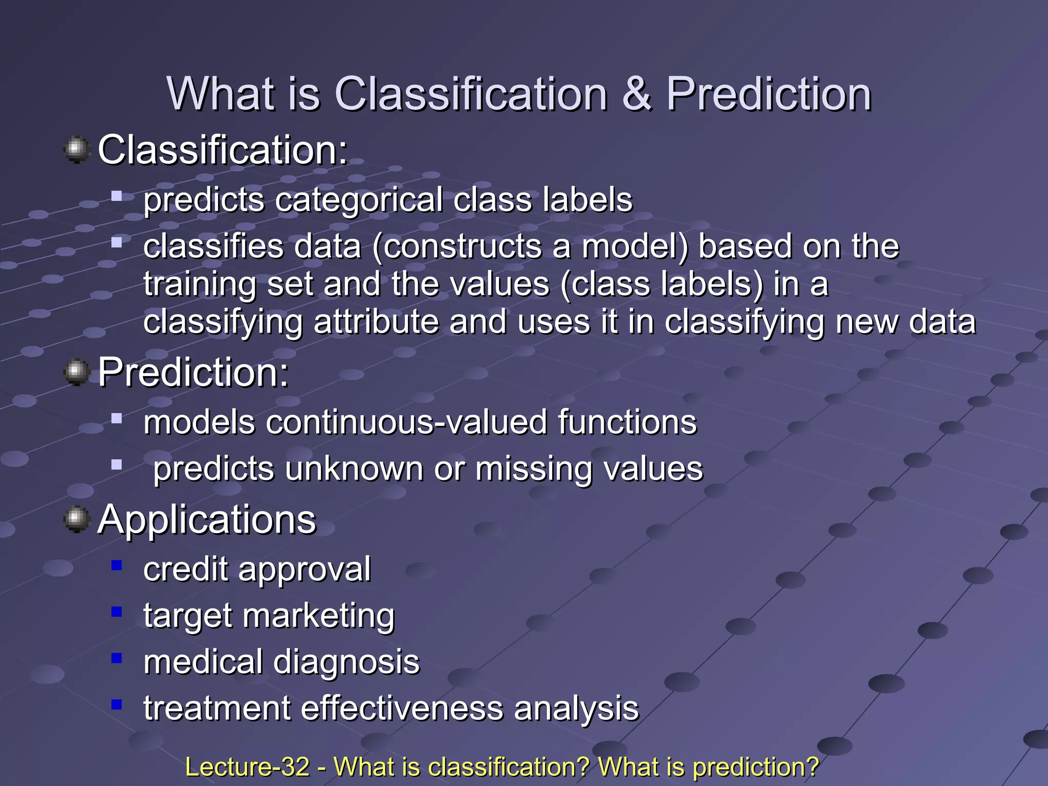
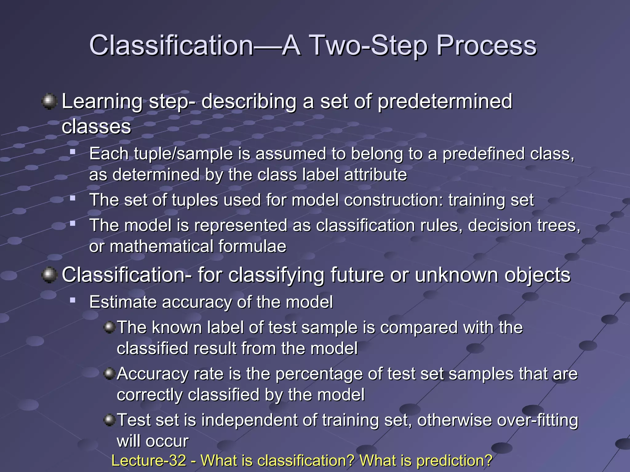
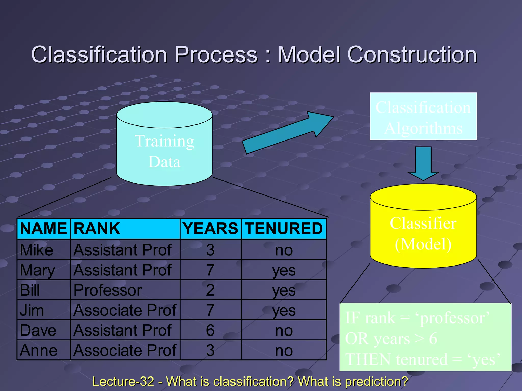
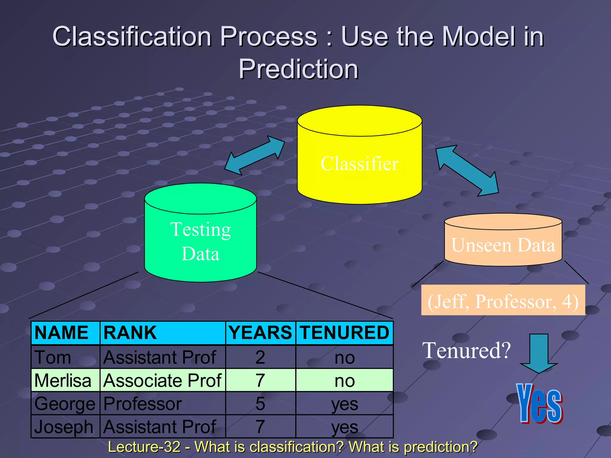


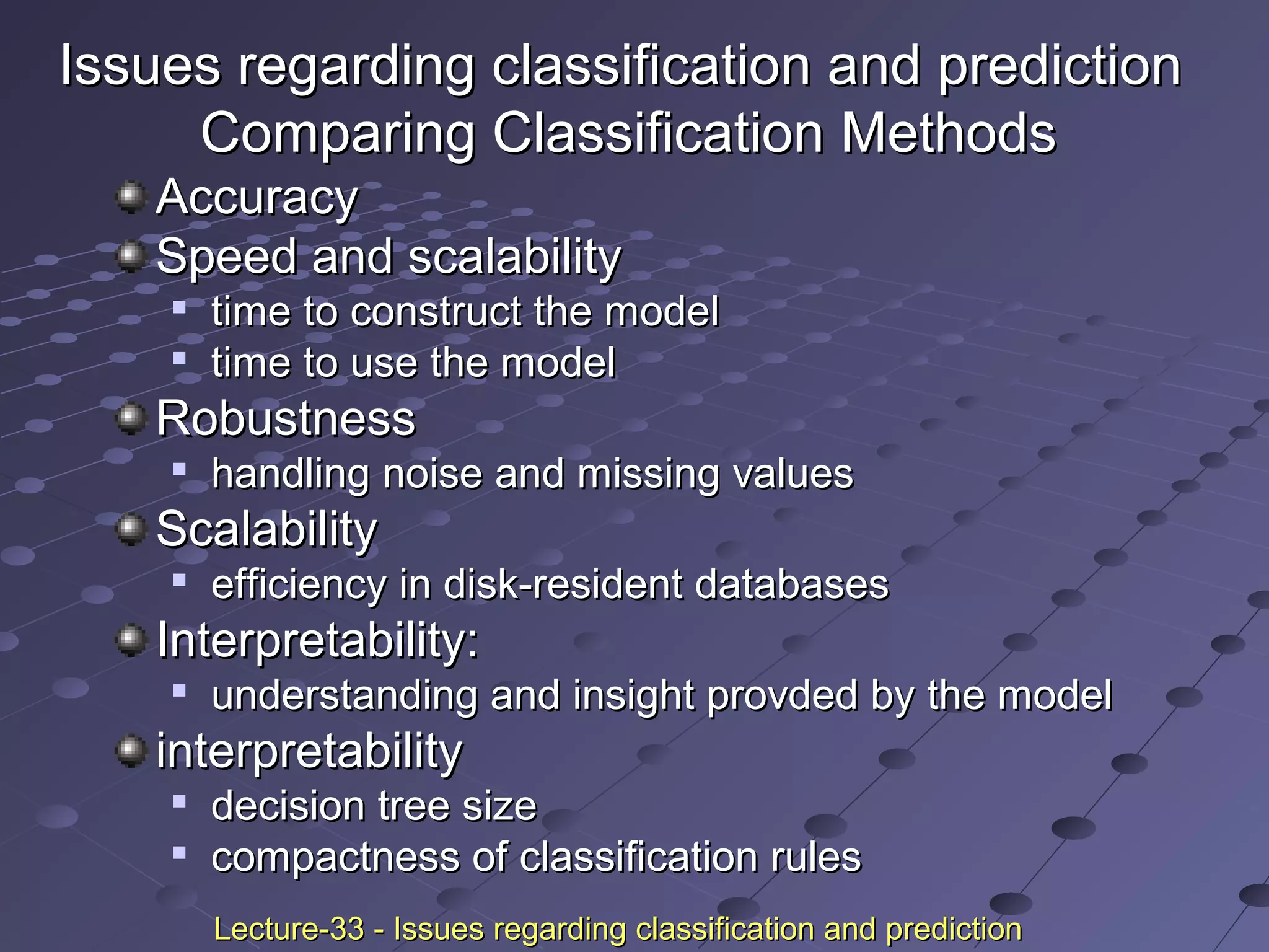


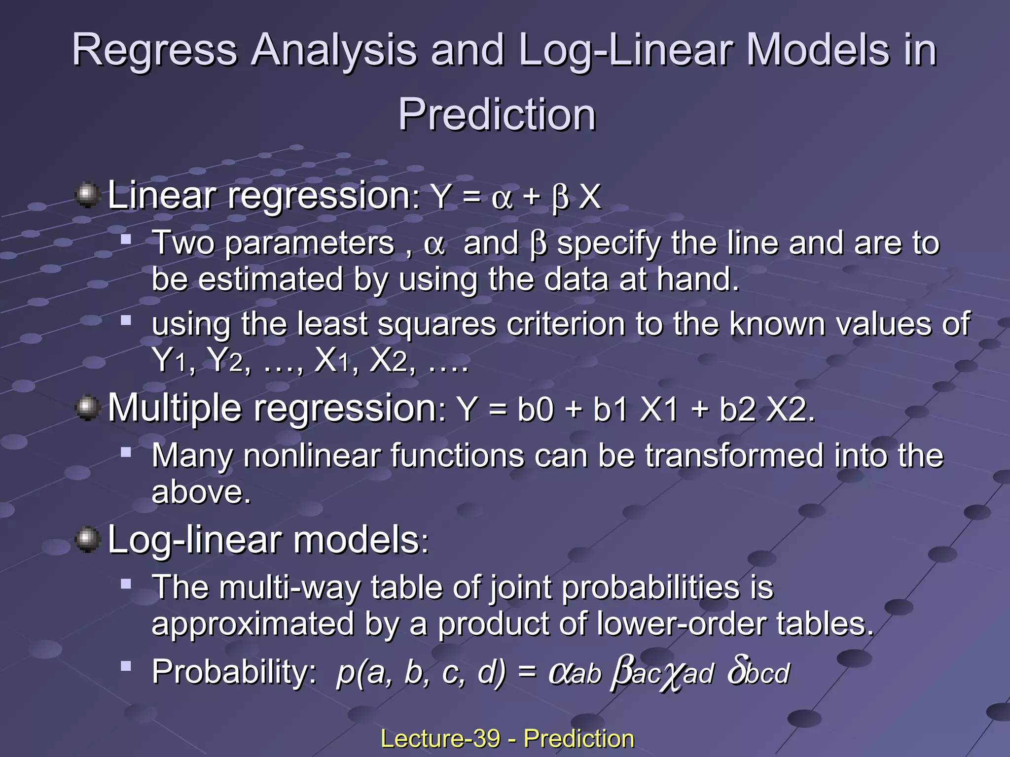
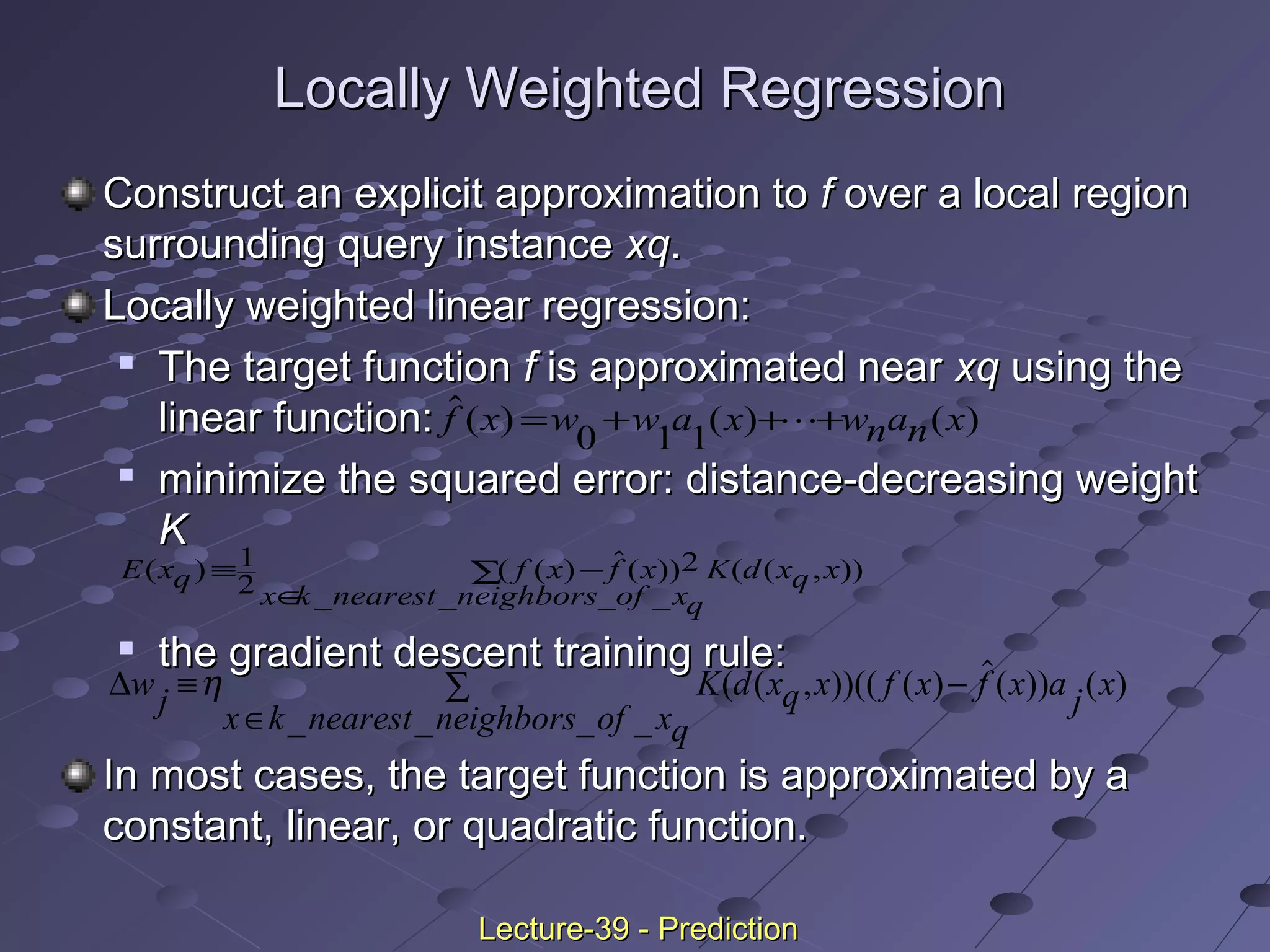
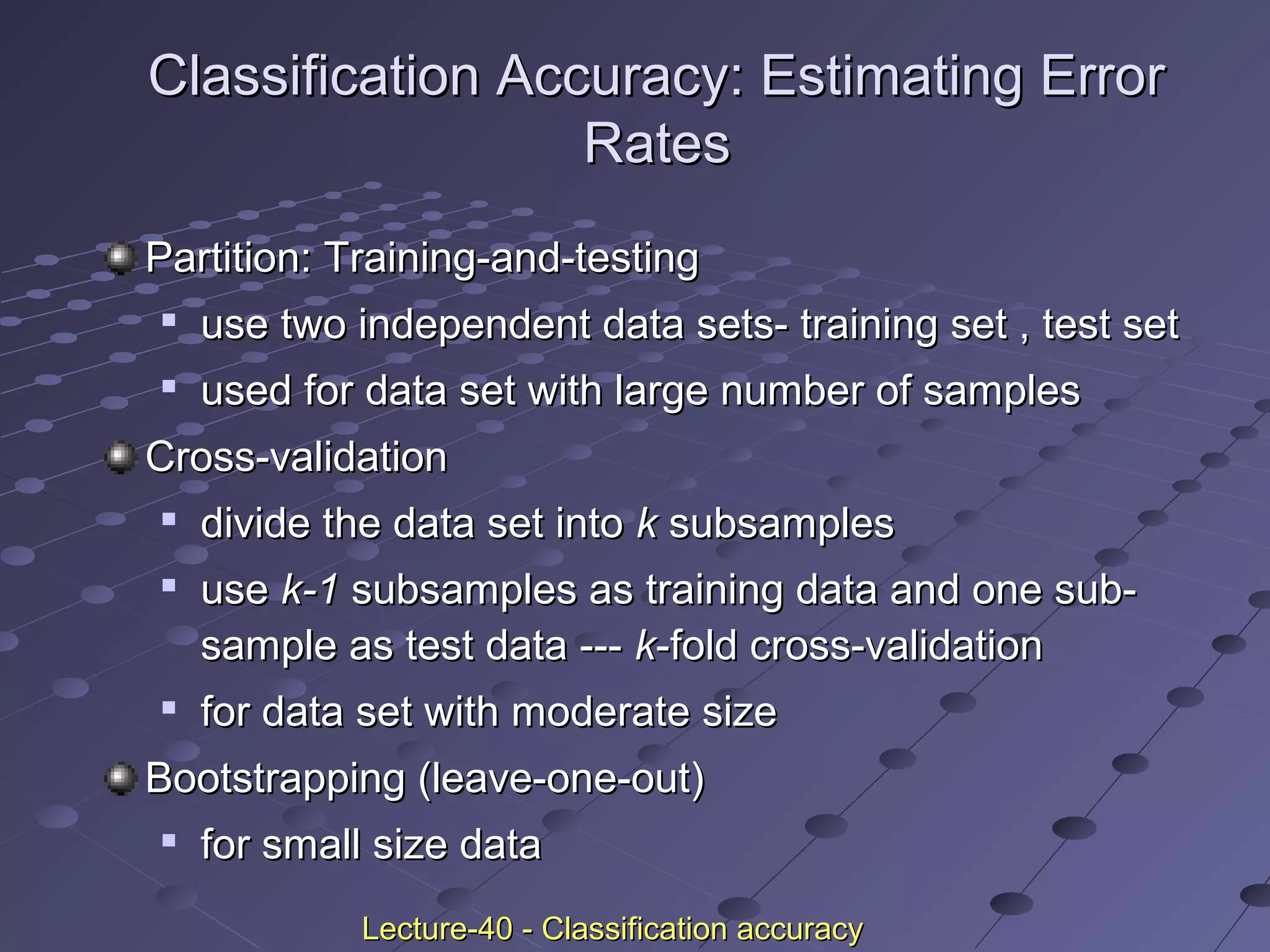
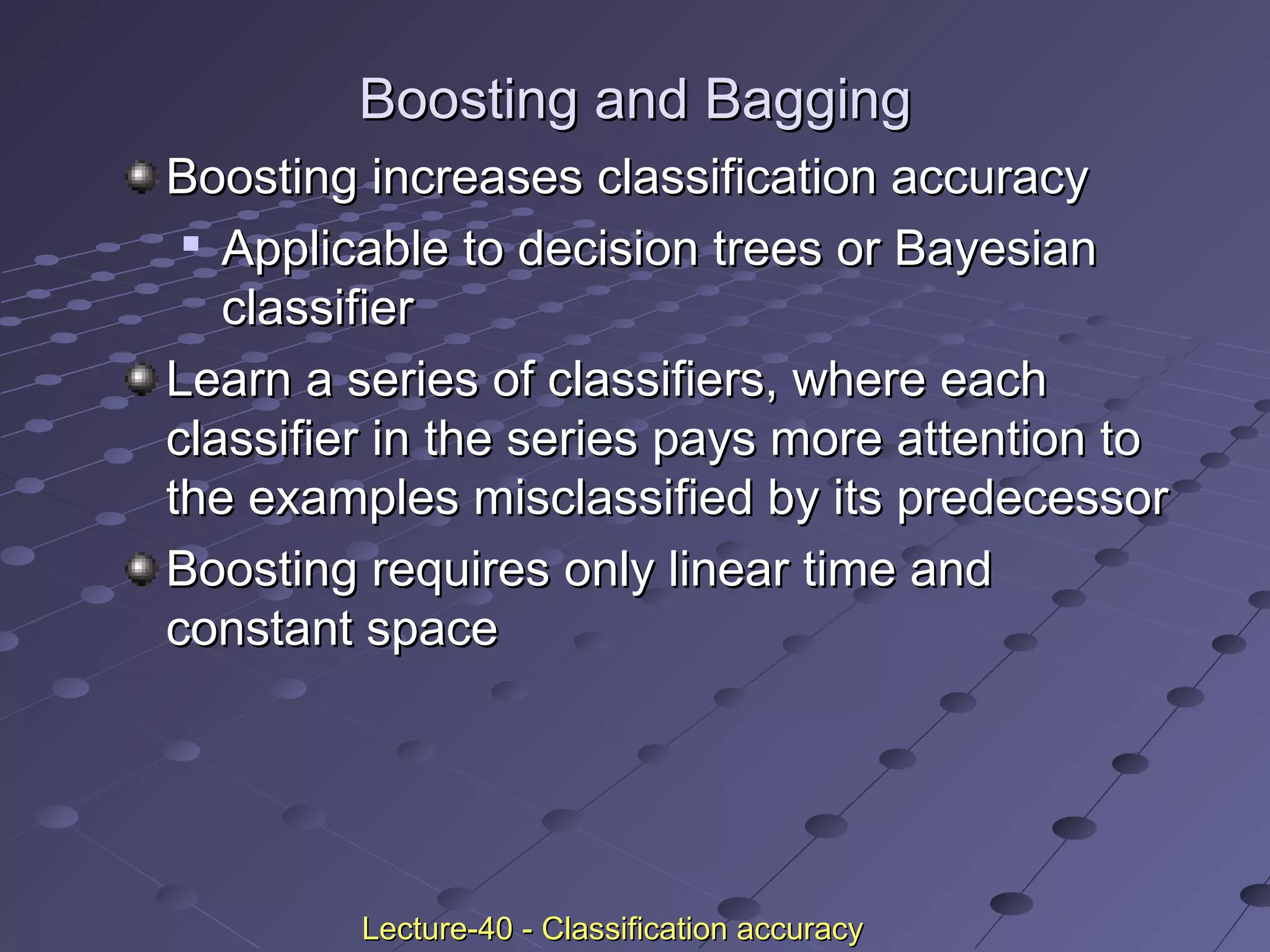

This document discusses classification and prediction. Classification predicts categorical class labels by classifying data based on a training set and class labels. Prediction models continuous values and predicts unknown values. Some applications are credit approval, marketing, medical diagnosis, and treatment analysis. Classification involves a learning step to describe classes and a classification step to classify new data. Prediction involves estimating accuracy by comparing test results to known labels. Issues with classification and prediction include data preparation, comparing methods, and decision tree induction algorithms.