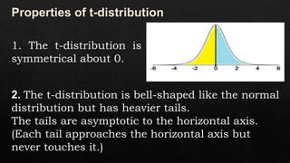
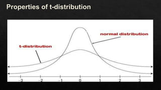
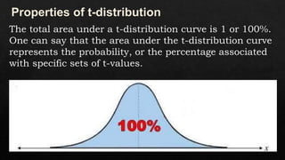
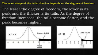
When we know the standard deviation of the population,
we can compute a z-score and use the normal
distribution to evaluate probabilities.
But sample sizes are sometimes small, and often we do
not know the standard deviation of the population.
When either of these problems occurs, the solution is to
use a different distribution.
It is probability distribution that is used to estimate
population parameters when the sample size is small (𝑖. 𝑒.
𝑠𝑎𝑚𝑝𝑙𝑒 𝑠𝑖𝑧𝑒 < 30) and/or when the population variance is
unknown.
It was developed by William Sealy Gosset in 1908. He used the
pseudonym or pen name “Student” when he published his paper
which describes the distribution. That is why it is called
“Student’s t-distribution”.
In the problem he analyzed, the sample size might be as low as
three.
1. The t-distribution is
symmetrical about 0.
2. The t-distribution is bell-shaped like the normal
distribution but has heavier tails.
The tails are asymptotic to the horizontal axis.
(Each tail approaches the horizontal axis but
never touches it.)
The total area under a t-distribution curve is 1 or 100%.
One can say that the area under the t-distribution curve
represents the probability, or the percentage associated
with specific sets of t-values.
The lesser the degree of freedom, the lower is its
peak and the thicker is its tails. As the degree of
freedom increases, the tails become flatter, and the
peak becomes higher.
illustrating the t-distribution.pptx

illustrating the t-distribution.pptx

  • 2.
    When we knowthe standard deviation of the population, we can compute a z-score and use the normal distribution to evaluate probabilities. But sample sizes are sometimes small, and often we do not know the standard deviation of the population. When either of these problems occurs, the solution is to use a different distribution.
  • 3.
    It is probabilitydistribution that is used to estimate population parameters when the sample size is small (𝑖. 𝑒. 𝑠𝑎𝑚𝑝𝑙𝑒 𝑠𝑖𝑧𝑒 < 30) and/or when the population variance is unknown. It was developed by William Sealy Gosset in 1908. He used the pseudonym or pen name “Student” when he published his paper which describes the distribution. That is why it is called “Student’s t-distribution”. In the problem he analyzed, the sample size might be as low as three.
  • 5.
    1. The t-distributionis symmetrical about 0. 2. The t-distribution is bell-shaped like the normal distribution but has heavier tails. The tails are asymptotic to the horizontal axis. (Each tail approaches the horizontal axis but never touches it.)
  • 7.
    The total areaunder a t-distribution curve is 1 or 100%. One can say that the area under the t-distribution curve represents the probability, or the percentage associated with specific sets of t-values.
  • 8.
    The lesser thedegree of freedom, the lower is its peak and the thicker is its tails. As the degree of freedom increases, the tails become flatter, and the peak becomes higher.