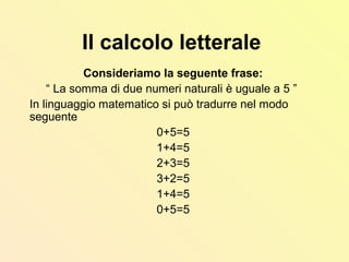
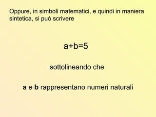
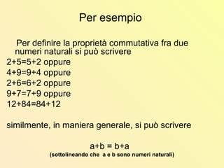
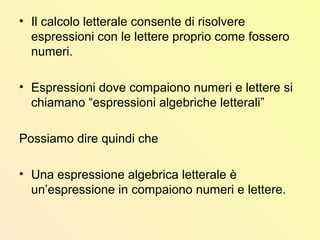
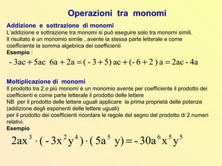
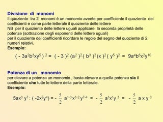
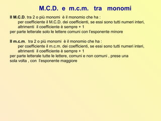
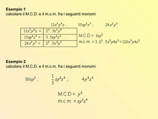
The document provides examples and exercises on writing linear equations in standard form, slope-intercept form, and two-point form. It discusses transforming equations between these forms and finding the slope and y-intercept. Examples are provided for writing equations of lines given the slope and a point, or two points. Exercises have students write equations of lines through points or with given slope, identifying slopes and y-intercepts of lines, and sketching line graphs.
This document discusses key concepts related to finding zeros of polynomial functions including:
1) The factor theorem, which states that a polynomial x - k is a factor of a function f(x) if and only if f(k) = 0.
2) The rational zeros theorem, which gives possible rational zeros based on the factors of the leading coefficient and constant term.
3) The fundamental theorem of algebra, which states that every polynomial of degree n has n complex zeros and examples of finding functions based on given zeros.
4) The conjugate zeros theorem, which states that if z = a + bi is a zero, then z = a - bi is also a zero for polynomials with real coefficients.
5
O documento contém várias perguntas e respostas sobre álgebra, incluindo a soma dos primeiros 20 números pares, graus de monômios, divisão, verdadeiro ou falso sobre números naturais e reais, dizimas periódicas, definição de álgebra, grau de polinomios, soma de perímetros e quais números são naturais.
Matemática - Exercícios Resolvidos de FatoraçãoJoana Figueredo
O documento apresenta uma série de exercícios de fatoração de expressões algébricas. As respostas mostram os passos para fatorar cada expressão, isolando os termos comuns e obtendo a forma fatorada final.
This document provides an overview of multiples, factors, least common multiples (LCM), highest common factors (HCF), prime numbers, and divisibility rules for numbers 2, 3, and 5 in a 7th grade mathematics chapter. It defines key terms, provides examples of finding multiples, factors, LCM, HCF, and discusses prime vs. composite numbers. Evaluation questions and group work assessing these concepts are assigned, along with homework reviewing common multiples, LCM, common factors, HCF, and listing prime numbers.
Absolute value functions have a V-shape and model situations involving distance or edges. The graph can be transformed by changing the slope (a), shifting the vertex horizontally (h), or shifting the vertex vertically (k). To graph, identify the vertex and axis of symmetry, then use the slope to sketch the right side and symmetry to complete the left. Writing the equation involves identifying the vertex (h, k) and slope (a).
Complex numbers and quadratic equationsriyadutta1996
The document discusses complex numbers and their properties. It defines i as the square root of -1 and shows that complex numbers can be written in the form a + bi, where a and b are real numbers. It describes how to add, subtract, multiply and divide complex numbers. It also discusses conjugates, moduli, and solving quadratic equations with complex number solutions.
1. Determina as condições para que denominadores de frações algébricas não sejam nulos.
2. Simplifica a fração 1a25/b62a30 para a = -1 e b = 4, obtendo o valor 4.
3. Indica que Carol e Luís foram os únicos alunos a simplificarem corretamente as frações algébricas.
Imaginary numbers are square roots of negative real numbers that were introduced to allow taking the square root of negatives. An example of an imaginary number is 2i√6, where i represents the imaginary unit. Imaginary numbers can be added, subtracted, multiplied, and divided like real numbers. When squared, imaginary numbers follow a repeating sequence of i, -1, -i, 1. Though sometimes complex, imaginary numbers serve an important purpose and are generally easy to work with through practice and logical thinking.
The document defines and provides examples of different types of matrices such as square, diagonal, identity, and zero matrices. It also discusses matrix operations like addition, subtraction, scalar multiplication, and matrix multiplication. Key properties of these operations such as commutativity, associativity, and invertibility are covered. Matrix transpose and elementary row operations are also introduced.
This document discusses finding the slope of a line from two points or an equation. It provides the slope formula and explains how to calculate slope given two points on a line. It also discusses horizontal and vertical lines, which have slopes of 0 and undefined, respectively. The document shows how to find the slope of a line from its equation by solving for y and taking the coefficient of x. It concludes by explaining how to determine if two lines are parallel, perpendicular, or neither based on the equality or product of their slopes. Examples are provided to demonstrate these concepts.
This document proves two trigonometric identities:
1) sin(a+b)=sin(a)cos(b)+cos(a)sin(b)
2) sin(a-b)=sin(a)cos(b)-cos(a)sin(b)
It does so by taking the left-hand side of each identity and mathematically manipulating it until it equals the right-hand side. Several steps of algebraic manipulation and trigonometric properties are used in each proof.
This document introduces methods for solving quadratic equations beyond factoring, including the square root property, completing the square, and the quadratic formula. It discusses how to determine the number and type of solutions based on the discriminant. The key steps are presented for solving quadratics, graphing quadratic functions as parabolas, and finding the domain and range. Piecewise-defined quadratic functions are also explained.
O documento discute tópicos de Geometria Analítica, incluindo coordenadas cartesianas no plano, área de triângulos, condição de alinhamento de pontos, equação geral da reta e outros.
A matrix is a set of elements organized into rows and columns. Basic matrix operations include addition, subtraction, and multiplication. A matrix can be multiplied by another matrix if the number of columns of the first equals the number of rows of the second. The determinant of a matrix is a value that is used to determine properties of the matrix such as invertibility. Cramer's rule can be used to solve systems of linear equations involving matrices.
This document provides examples for solving simultaneous linear equations using three methods: substitution, elimination, and graphical approach. It also presents sample problems for students to practice solving simultaneous equations using these three methods. The document aims to teach students how to solve simultaneous linear equations after covering the three solution methods.
The document discusses solving quadratic equations by factoring. It provides examples of factoring quadratic expressions into linear factors and setting each factor equal to 0 to solve for the roots. The key steps are: 1) write the equation in standard form, 2) factor completely, 3) set each factor equal to 0, 4) solve for the roots, and 5) check the solutions. It also provides examples of using this method to solve word problems involving quadratic equations.
O documento apresenta os conceitos básicos de logaritmos, incluindo sua definição, condições de existência, propriedades operatórias e aplicações em equações logarítmicas.
The document is a presentation on polynomials. It defines a polynomial as an expression that can contain constants, variables, and exponents, but cannot contain division by a variable. It discusses the key characteristics of polynomials including their degree, standard form, zeros, factoring, and algebraic identities. Examples are provided to illustrate different types of polynomials like monomials, binomials, trinomials, and how to add, subtract, multiply and divide polynomials.
Solving systems of linear equations by graphing lectureKaiya Duppins
This document discusses solving systems of linear equations by graphing. It defines a system of linear equations as two or more equations containing at least one variable. It explains that to solve a system by graphing, each equation should be written in slope-intercept form and then graphed on the same set of axes. The type of solution can be determined by examining the graphs - one solution if the lines intersect, no solution if the lines are parallel, or infinitely many solutions if the lines coincide. It provides examples to illustrate each type of solution and explains that the point of intersection or coinciding point(s) will be the solution(s) to plug back into the original system to check.
The history and development of matrix theory is summarized as follows:
1) The term "matrix" was introduced in 1850 by James Joseph Sylvester to describe rectangular arrays of numbers or expressions arranged in rows and columns.
2) The founder of modern matrix theory is considered to be Arthur Cayley, who in the 1850s introduced concepts such as inverse matrices and matrix multiplication.
3) Important developments in matrix theory continued throughout the 19th and 20th centuries, including the discovery by Arthur Cayley and William Hamilton of unique properties of matrices.
The document discusses polar coordinates and graphs. Polar coordinates (r, θ) can be used to specify the location of a point P by giving the distance r from the origin and the angle θ. Conversion formulas allow changing between polar (r, θ) and rectangular (x, y) coordinates. Polar equations relate r and θ, and common ones like r = c (a circle) and θ = c (a line) are examined. Graphing polar equations involves plotting the r and θ values specified by the equation.
1) A radiciação é a operação inversa da potenciação. Radicais podem ter índices pares ou ímpares, afetando o número de raízes de um número.
2) Existem propriedades para simplificar radicais, como quando o índice e expoente são divisíveis ou quando o expoente é múltiplo do índice.
3) Pode-se adicionar, subtrair, multiplicar e dividir radicais semelhantes, isto é, com mesmo índice e radicando. Para operações com radic
The document introduces sequences and series. It discusses revising linear and quadratic sequences. It introduces arithmetic sequences, which have a constant difference between terms, and geometric sequences, which have a constant ratio between terms. It provides examples of determining the general term and specific terms of arithmetic and geometric sequences. Formulas are given for the general terms of both arithmetic (Tn = a + (n-1)d) and geometric (Tn = arn-1) sequences.
2. Il calcolo letterale
Consideriamo la seguente frase:
“ La somma di due numeri naturali è uguale a 5 ”
In linguaggio matematico si può tradurre nel modo
seguente
0+5=5
1+4=5
2+3=5
3+2=5
1+4=5
0+5=5
3. Oppure, in simboli matematici, e quindi in maniera
sintetica, si può scrivere
a+b=5
sottolineando che
a e b rappresentano numeri naturali
4. Se i calcoli vengono eseguiti con
le lettere invece che con i numeri,
si può costruire una forma più
generale rispetto ad un semplice
esempio numerico.
5. Per esempio
Per definire la proprietà commutativa fra due
numeri naturali si può scrivere
2+5=5+2 oppure
4+9=9+4 oppure
2+6=6+2 oppure
9+7=7+9 oppure
12+84=84+12
similmente, in maniera generale, si può scrivere
a+b = b+a
(sottolineando che a e b sono numeri naturali)
6. • Il calcolo letterale consente di risolvere
espressioni con le lettere proprio come fossero
numeri.
• Espressioni dove compaiono numeri e lettere si
chiamano “espressioni algebriche letterali”
Possiamo dire quindi che
• Una espressione algebrica letterale è
un’espressione in compaiono numeri e lettere.
7. Esempi
in generale la somma di due numeri
qualsiasi si può scrivere
in generale il prodotto di due numeri
qualsiasi si può scrivere
x x y
oppure, ancora meglio,
(per non confondere il segno di moltiplicazione con la lettera x)
yx +
yx ⋅
8. Il doppio di quattro in linguaggio
matematico si può scrivere
Il doppio di dodici in linguaggio
matematico si può scrivere
Il doppio di un numero in linguaggio
matematico si può scrivere
Dove x rappresenta un numero qualsiasi.
42⋅
122⋅
x⋅2
9. La metà di 8 in linguaggio matematico si può
scrivere
La metà di 13 in linguaggio matematico si
può scrivere
La metà di un numero in linguaggio
matematico si può scrivere
Dove x rappresenta un numero qualsiasi.
2
8
2
13
2
x
10. Consideriamo un rettangolo e
indichiamo con x il lato maggiore e con y
il lato minore.
Quanto vale il perimetro?
Esercizio
Il perimetro vale
11. L'espressione letterale più
semplice è il monomio.
Definizione di monomio
“Un monomio è una espressione algebrica di numeri e lettere in cui
compare soltanto l’operazione di moltiplicazione e gli esponenti delle
lettere sono numeri naturali.”
Possiamo anche dire:
“Un monomio è una espressione algebrica letterale in cui compare solo
l’operazione di moltiplicazione e gli esponenti delle lettere sono numeri
naturali.”
Esempio : -2a3
b4
x6
; xyt ; a3
b2
c 5a3
7b4
x2
Un monomio si dice nullo quando la parte numerica è uguale a 0
Un monomio si dice ridotto in forma normale quando è scritto come
prodotto di un solo numero e una o più lettere tutte diverse tra loro.
5
3
12. Quando un monomio è ridotto in forma normale:
La parte numerica si dice coefficiente numerico
Le lettere costituiscono la parte letterale.
Esempio :
-2a3
b4
x6
è ridotto in forma normale
(-2 rappresenta il coefficiente numerico e a3
b4
x6
rappresenta la parte letterale )
5a3
3b4
x2
b non è ridotto in forma normale;
(per ridurlo in forma normale dobbiamo scrivere 30 a3
b5
x)
13. Grado di un monomio: è la somma degli esponenti
di tutte le lettere che compaiono nel monomio
Esempio : 4 a3
b2
c è un monomio di grado 6 ,
perché 3+2+1 = 6
Monomi simili : due o più monomi sono simili
quando hanno la stessa parte letterale
Esempio : 2ab ; - 3ab ; 5ba;
Monomi opposti : sono due monomi simili , ma con
coefficienti opposti
Esempio : - 2ab e + 2ab
14. Operazioni tra monomi
Addizione e sottrazione di monomi
L’addizione e sottrazione tra monomi si può eseguire solo tra monomi simili.
Il risultato è un monomio simile , avente la stessa parte letterale e come
coefficiente la somma algebrica dei coefficienti
Esempio :
Moltiplicazione di monomi
Il prodotto tra 2 o più monomi è un monomio avente per coefficiente il prodotto dei
coefficienti e come parte letterale il prodotto delle lettere
NB per il prodotto delle lettere uguali applicare la prima proprietà delle potenze
(addizione degli esponenti delle lettere uguali)
per il prodotto dei coefficienti ricordare le regole del segno del prodotto di 2 numeri
relativi.
Esempio
5565423
yx30a-y)5a()y3x-(2ax =⋅⋅
4a-2aca)26(-ac5)3-(2a6a5ac3ac- =+++=++
15. Divisione di monomi
Il quoziente tra 2 monomi è un monomio avente per coefficiente il quoziente dei
coefficienti e come parte letterale il quoziente delle lettere
NB per il quoziente delle lettere uguali applicare la seconda proprietà delle
potenze (sottrazione degli esponenti delle lettere uguali)
per il quoziente dei coefficienti ricordare le regole del segno del quoziente di 2
numeri relativi.
Esempio:
Potenza di un monomio
per elevare a potenza un monomio , basta elevare a quella potenza sia il
coefficiente che tutte le lettere della parte letterale.
Esempio:
16. M.C.D. e m.c.m. tra monomi
Il M.C.D. tra 2 o più monomi è il monomio che ha :
per coefficiente il M.C.D. dei coefficienti, se essi sono tutti numeri interi,
altrimenti il coefficiente è sempre + 1
per parte letterale solo le lettere comuni con l’esponente minore
Il m.c.m. tra 2 o più monomi è il monomio che ha :
per coefficiente il m.c.m. dei coefficienti, se essi sono tutti numeri interi,
altrimenti il coefficiente è sempre + 1
per parte letterale tutte le lettere, comuni e non comuni , prese una
sola volta , con l’esponente maggiore
17. Esempio 1
calcolare il M.C.D. e il m.c.m. fra i seguenti monomi
Esempio 2
calcolare il M.C.D. e il m.c.m. fra i seguenti monomi
18. POLINOMI
DEFINIZIONE DI POLINOMIO
Un polinomio è dato dalla somma algebrica di 2 o più monomi non simili
(i monomi che compaiono in un polinomio si dicono TERMINI del
polinomio)
Esempio : 2a + 3b ; 4axy – 3x + 5a
GRADO COMPLESSIVO DI UN POLINOMIO : è il grado del suo
monomio di grado maggiore
Esempio : il polinomio ( 3a4
xy5
– 2x)
ha grado complessivo 10 , perché tra i 2 monomi che
formano il polinomio , il 1° monomio ha grado maggiore e
vale 10
19. POLINOMIO ORDINATO IN MODO CRESCENTE RISPETTO A UNA LETTERA
se i suoi termini sono disposti in modo tale che gli esponenti di
quella lettera sono in ordine crescente
Esempio : 8x5
y – 5x6
y2
+ 7 x8
è ordinato secondo potenze crescenti di x
POLINOMIO ORDINATO IN MODO DECRESCENTE RISPETTO A UNA LETTERA
se i suoi termini sono disposti in modo tale che gli esponenti di
quella lettera sono in ordine decrescente
Esempio : 8x6
y3
– 5x2
y2
+ 7 xy1
20. POLINOMIO COMPLETO RISPETTO AD UNA LETTERA
se per tale lettera si presentano tutte le potenze dal grado massimo fino al
grado 0
Esempio : 2a3
+ a2
– 7a + 8
POLINOMIO OMOGENEO
se tutti i suoi termini hanno lo stesso grado
Esempio : 2a3
+ a2
b – 7ab2
+ 8 b3
21. OPERAZIONI TRA POLINOMI
ADDIZIONE E SOTTRAZIONE TRA POLINOMI
Per addizionare o sottrarre 2 o più polinomi si scrivono uno di seguito all’altro
eliminando le parentesi e sommando i termini simili
Per eliminare le parentesi si applicano le regole già note:
se la parentesi è preceduta da un segno + ,
i termini in essa contenuti non cambiano segno
se la parentesi è preceduta da un segno - ,
i termini in essa contenuti cambiano segno
esempio
( 2a3
+ a2
– 25a + 12 ) = 2a3
+ a2
– 25a + 12
- ( 2a3
+ a2
– 25a + 12 ) = - 2a3
- a2
+25a – 12
22. Eseguire la seguente somma algebrica di polinomi:
eliminiamo le parentesi
Semplifichiamo i monomi opposti 5b e -5b; +3a e -3a
Sommiamo i monomi simili e otteniamo il polinomio cercato.
5ab)(6a-2b)-(3a-5b)(3a5b)(2a 22
=++−++
5ab6a-2b3a-5b3a5b2a 22
=+−+−++
2
a-b2a +
23. MOLTIPLICAZIONE DI UN MONOMIO PER UN POLINOMIO
Basta applicare la proprietà distributiva della moltiplicazione , moltiplicando ogni
termine del polinomio per il monomio ( ricordando la proprietà della moltiplicazione
tra potenze con basi uguali e la regola dei segni della moltiplicazione)
Esempio : ( - 3a2b ) .
( 3a - b + 5ab ) = - 9 a3
b + 3 a2
b2
– 15 a3
b2
DIVISIONE DI UN POLINOMIO PER UN MONOMIO
Basta applicare la proprietà distributiva della divisione, dividendo ogni termine del
polinomio per il monomio ( ricordando la proprietà della divisione tra potenze con
basi uguali e la regola dei segni della divisione )
Esempio 1 (12a2
– 9ab + 6a ) : ( - 3 a ) = - 4 a + 3b – 2
Esempio 2 ( x + 3y – 4 ) : 2x =
24. MOLTIPLICAZIONE TRA DUE POLINOMI
Basta moltiplicare ogni termine del primo polinomio per ogni termine del
secondo polinomio
Esempio :
( 2a - 3b ) .
( -3ab + 5ax + 1 ) = - 6a2
b + 10 a2
x + 2a + 9ab2
- 15abx – 3b