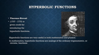
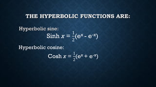
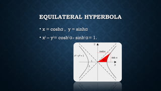
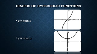
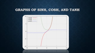
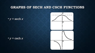
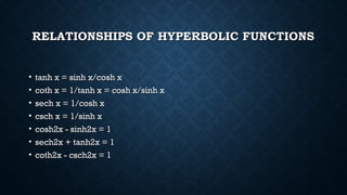
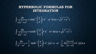
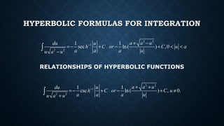
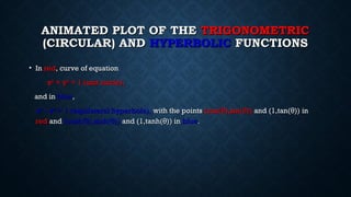
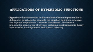
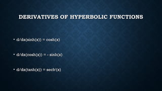
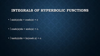
a presentetion slide about hyperbolic functions
source: https://www.slideshare.net/farhanashaheen1/hyperbolic-functions-dfs?qid=2e8a572a-39b0-4d08-9dac-f0abf13fe9f5&v=&b=&from_search=1
Hyperbolic functions are useful in mathematics and physics. The main hyperbolic functions are the hyperbolic sine, cosine, and tangent. Hyperbolic curves include the catenary curve, which describes the shape of a hanging chain and is modeled by the hyperbolic cosine function. Hyperbolic functions are applied in areas like physics, differential equations, and special relativity.
The document provides an introduction to partial differential equations (PDEs). Some key points:
- PDEs involve functions of two or more independent variables, and arise in physics/engineering problems.
- PDEs contain partial derivatives with respect to two or more independent variables. Examples of common PDEs are given, including the Laplace, wave, and heat equations.
- The order of a PDE is defined as the order of the highest derivative. Methods for solving PDEs through direct integration and using Lagrange's method are briefly outlined.
Partial Differential Equation plays an important role in our daily life.In mathematics, a partial differential equation (PDE) is a differential equation that contains unknown multivariable functions and their partial derivatives. PDEs are used to formulate problems involving functions of several variables, and are either solved by hand, or used to create a computer model. A special case is ordinary differential equations (ODEs), which deal with functions of a single variable and their derivatives.
PDEs can be used to describe a wide variety of phenomena such as sound, heat, diffusion, electrostatics, electrodynamics, fluid dynamics, elasticity, or quantum mechanics. These seemingly distinct physical phenomena can be formalised similarly in terms of PDEs. Just as ordinary differential equations often model one-dimensional dynamical systems, partial differential equations often model multidimensional systems. PDEs find their generalisation in stochastic partial differential equations.
This document discusses topics in partial differentiation including:
1) The geometrical meaning of partial derivatives as the slope of the tangent line to a surface.
2) Finding the equation of the tangent plane and normal line to a surface.
3) Taylor's theorem and Maclaurin's theorem for functions with two variables, which can be used to approximate functions and calculate errors.
The document discusses convergence of sequences and power series. It defines convergence of a sequence and states that the limit of a convergent sequence is unique. It also discusses Taylor series and Laurent series, stating that if a function f(z) is analytic inside a circle C with center z0, its Taylor series representation about z0 will converge to f(z) for all z inside C. Similarly, if f(z) is analytic in an annular region bounded by two concentric circles, its Laurent series will represent f(z) in that region.
This presentation will be very helpful to learn about system of linear equations, and solving the system.It includes common terms related with the lesson and using of Cramer's rule.
Please download the PPT first and then navigate through slide with mouse clicks.
Gauss Forward And Backward Central Difference Interpolation Formula Deep Dalsania
This PPT contains the topic called Gauss Forward And Backward Central Difference Interpolation Formula of subject called Numerical and Statistical Methods for Computer Engineering.
This document provides an overview of the topics covered in the Numerical Methods course CISE-301. It discusses:
- Numerical methods as algorithms used to obtain numerical solutions to mathematical problems when analytical solutions do not exist or are difficult to obtain.
- Specific topics that will be covered, including solution of nonlinear equations, linear equations, curve fitting, interpolation, numerical integration, differentiation, and ordinary and partial differential equations.
- An introduction to Taylor series and how they can be used to approximate functions, along with examples of Maclaurin series expansions.
- How numerical representations of real numbers like floating point can lead to rounding errors, and the concepts of accuracy and precision in numerical calculations.
The document defines and discusses inverse trigonometric functions. It defines them as the inverses of trigonometric functions like sine, cosine, and tangent, with restricted domains. Some key properties discussed include identities, derivatives, and integrals of inverse trigonometric functions. Graphs of inverse sine and cosine are reflections of sine and cosine about the line y=x.
Integration is used in physics to determine rates of change and distances given velocities. Numerical integration is required when the antiderivative is unknown. It involves approximating the definite integral of a function as the area under its curve between bounds. The Trapezoidal Rule approximates this area using straight lines between points, while Simpson's Rule uses quadratic or cubic functions, achieving greater accuracy with fewer points. Both methods involve dividing the area into strips and summing their widths multiplied by the function values at strip points.
Integration Made Easy!
The derivative of a function can be geometrically interpreted as the slope of the curve of the mathematical function f(x) plotted as a function of x. But its implications for the modeling of nature go far deeper than this simple geometric application might imply. After all, you can see yourself drawing finite triangles to discover slope, so why is the derivative so important? Its importance lies in the fact that many physical entities such as velocity, acceleration, force and so on are defined as instantaneous rates of change of some other quantity. The derivative can give you a precise intantaneous value for that rate of change and lead to precise modeling of the desired quantity.
This document discusses sequences and their limits. Some key points:
- A sequence is a list of numbers written in a definite order. It can be thought of as a function with domain the positive integers.
- The limit of a sequence is defined as the number L such that the terms of the sequence can be made arbitrarily close to L by choosing a sufficiently large term.
- A sequence converges if it has a finite limit, and diverges if its terms approach infinity. Bounded monotonic sequences are guaranteed to converge.
- Properties of sequence limits parallel those of limits of functions, including laws of limits and the ability to pass limits inside continuous functions.
First order linear differential equationNofal Umair
1. A differential equation relates an unknown function and its derivatives, and can be ordinary (involving one variable) or partial (involving partial derivatives).
2. Linear differential equations have dependent variables and derivatives that are of degree one, and coefficients that do not depend on the dependent variable.
3. Common methods for solving first-order linear differential equations include separation of variables, homogeneous equations, and exact equations.
3 examples of PDE, for Laplace, Diffusion of Heat and Wave function. A brief definition of Fouriers Series. Slides created and compiled using LaTeX, beamer package.
This document provides examples and explanations of double integrals. It defines a double integral as integrating a function f(x,y) over a region R in the xy-plane. It then gives three key points:
1) To evaluate a double integral, integrate the inner integral first treating the other variable as a constant, then integrate the outer integral.
2) The easiest regions to integrate over are rectangles, as the limits of integration will all be constants.
3) For non-rectangular regions, the limits of integration may be variable, requiring more careful analysis to determine the limits for each integral.
The document discusses periodic functions and their properties. The key points are:
- A periodic function f(x) satisfies f(x) = f(x + T) for some fixed period T and all real x.
- Periodic functions repeat their values at intervals of their period, including integer multiples of the period.
- Functions are defined as even if f(-x) = f(x) and odd if f(-x) = -f(x).
- Several important formulas are provided for integrating exponential and trigonometric functions.
Integration by substitution is the chain rule in reverse.
NOTE: the final location is section specific. Section 1 (morning) is in SILV 703, Section 11 (afternoon) is in CANT 200
The document discusses the Mean Value Theorem, which states that if a function f(x) is continuous on the closed interval [a,b] and differentiable on the open interval (a,b), then there exists some value c in (a,b) such that:
f(b) - f(a) = f'(c)(b - a)
In other words, there is at least one point where the slope of the tangent line equals the slope of the secant line between points a and b. The document provides examples and illustrations to demonstrate how to apply the Mean Value Theorem.
This document provides information on several multivariable calculus topics:
1) Finding maxima and minima of functions of two variables using partial derivatives and the second derivative test.
2) Finding the tangent plane and normal line to a surface.
3) Taylor series expansions for functions of two variables.
4) Standard expansions for common functions like e^x, cosh(x), and tanh(x) using Maclaurin series.
5) Linearizing functions around a point using the tangent plane approximation.
6) Lagrange's method of undetermined multipliers for finding extrema with constraints.
This document contains multiple choice questions related to numerical methods. The questions cover topics like regular falsi method, Newton-Raphson method, numerical integration techniques like trapezoidal rule and Simpson's rule, and numerical differentiation techniques like forward and backward difference formulas. Numerical methods for solving differential equations like Euler's method and Runge-Kutta methods are also addressed.
1) The document discusses partial derivatives, which involve differentiating functions of two or more variables with respect to one variable while holding the others constant. It provides examples of computing first and second partial derivatives.
2) Implicit differentiation is introduced as a way to find partial derivatives of functions defined implicitly rather than explicitly. The chain rule is also discussed.
3) Methods are presented for finding partial derivatives of functions of two or three variables, including using implicit differentiation and the chain rule. Examples are provided to illustrate these concepts.
1) The document discusses differentiation and various techniques for taking derivatives of functions with respect to variables like x and y. This includes the derivative of sums, constants, products, quotients, exponentials, logarithms and inverse trigonometric functions.
2) Applications of differentiation like finding rates of change, tangents, normals, and stationary points are covered. Techniques for finding maximum/minimum values using derivatives are presented.
3) Series expansions like Maclaurin and Taylor series are introduced to approximate functions as polynomials. The concept of partial derivatives is defined for functions with two variables.
The document uses the ratio test to find the radius of convergence for two power series. For the first series, the ratio test gives an interval of convergence from -2 to 4, so the radius of convergence is 3. For the second series, the ratio test gives the interval of convergence as from -infinity to infinity, so the radius of convergence is infinite.
This document discusses Taylor series expansions. It defines Taylor series as the expansion of a complex function f(z) that is analytic inside and on a simple closed curve C in the z-plane. The Taylor series expresses f(z) as a power series centered at a point z0 within C. It provides examples of standard Taylor series expansions and worked illustrations of expanding various functions as Taylor series. The document also notes that the radius of convergence of a Taylor series is defined by the distance to the nearest singularity from the center point z0.
This document contains the syllabus for a course on Mathematical Methods taught according to the JNTU-Hyderabad new syllabus. It covers topics like matrices and linear systems, eigenvalues and eigenvectors, linear transformations, solution of nonlinear systems, curve fitting, numerical integration, Fourier series, and partial differential equations. The specific section summarized discusses numerical differentiation using forward, backward, and central differences. It also covers numerical integration techniques like the trapezoidal rule, Simpson's 1/3 rule, and Simpson's 3/8 rule.
MATLAB : Numerical Differention and IntegrationAinul Islam
This document describes numerical techniques for differentiation and integration. It discusses forward difference, central difference, and Richardson's extrapolation formulas for numerical differentiation. For numerical integration, it covers the trapezoidal rule and Simpson's rule. The trapezoidal rule approximates areas using trapezoids formed by the function values at interval points. Simpson's rule uses quadratic polynomials to approximate the function within each interval. Both methods converge to the true integral as the number of intervals increases.
In mathematics, hyperbolic functions are analogues of the ordinary trigonometric functions defined for the hyperbola rather than on the circle: just as the points form a circle with a unit radius, the points form the right half of the equilateral hyperbola.
This document provides information about Calculus 2, including lessons on indeterminate forms, Rolle's theorem, the mean value theorem, and differentiation of transcendental functions. It defines Rolle's theorem and the mean value theorem, provides examples of applying each, and discusses how Rolle's theorem can be used to find the value of c. It also defines inverse trigonometric functions and their derivatives. The document is for MATH 09 Calculus 2 and includes exercises for students to practice applying the theorems.
The document discusses the Schrodinger equation and methods to approximate solutions to it. It begins by defining the time-independent Schrodinger equation and its components. It then provides examples of writing out the Schrodinger equation for different chemical systems with varying numbers of electrons and nuclei. Approximation methods are needed because the Schrodinger equation can only be exactly solved for a few simple systems. Two approximation methods discussed are the variational method and perturbation theory. The variational method uses a trial wavefunction to variationally minimize the energy.
Hidden Symmetries and Their Consequences in the Hubbard Model of t2g ElectronsABDERRAHMANE REGGAD
(1) The Hubbard model for t2g electrons in transition metal oxides possesses novel hidden symmetries that have significant consequences.
(2) These symmetries prevent long-range spin order at non-zero temperatures and lead to an extraordinary simplification in exact diagonalization studies.
(3) Even with spin-orbit interactions included, the excitation spectrum remains gapless due to a continuous symmetry arising from the hidden symmetries.
Observational Parameters in a Braneworld Inlationary ScenarioMilan Milošević
This document describes a study of observational parameters in a braneworld inflationary scenario. It provides background on standard cosmological models, inflationary theory, and observational parameters measured by Planck. It then discusses tachyon inflation models and the Randall-Sundrum braneworld model. The study extends the RS model to include a dynamical radion field and examines the dynamics and observational predictions of tachyon inflation in this braneworld model through numerical simulations.
This document compares the performance of an LQR controller and PD controller for stabilizing a double inverted pendulum system. It first describes the nonlinear dynamics of a double inverted pendulum and derives its equations of motion. It then linearizes the system around the equilibrium point to obtain a state space model. Next, it analyzes the stability, controllability and observability of the linearized system. Finally, it implements both an LQR controller and PD controller in MATLAB/Simulink to control the double inverted pendulum and compare their performance with respect to the pendulum angles and cart position.
IJERD(www.ijerd.com)International Journal of Engineering Research and Develop...IJERD Editor
This document compares the performance of an LQR controller and PD controller for stabilizing a double inverted pendulum system. It first describes the nonlinear dynamics of a double inverted pendulum and derives its equations of motion. It then linearizes the system model around the equilibrium point and analyzes the stability, controllability, and observability of the linearized system. Finally, it compares the performance of an LQR controller and PD controller with respect to the pendulum angles and cart position using MATLAB simulations.
The International Journal of Engineering & Science is aimed at providing a platform for researchers, engineers, scientists, or educators to publish their original research results, to exchange new ideas, to disseminate information in innovative designs, engineering experiences and technological skills. It is also the Journal's objective to promote engineering and technology education. All papers submitted to the Journal will be blind peer-reviewed. Only original articles will be published.
The papers for publication in The International Journal of Engineering& Science are selected through rigorous peer reviews to ensure originality, timeliness, relevance, and readability.
Dumitru Vulcanov - Numerical simulations with Ricci flow, an overview and cos...SEENET-MTP
Lecture by prof. dr Dumitru Vulcanov (dean of the Faculty of Physics, West University of Timisoara, Romania) on October 21, 2010 at the Faculty of Science and Mathematics, Nis, Serbia.
This document is Scott Shermer's master's thesis on instantons and perturbation theory in the 1-D quantum mechanical quartic oscillator. It begins by reviewing the harmonic oscillator and perturbation theory. It then discusses non-perturbative phenomena like instantons and Borel resummation. The focus is on obtaining the ground state energy of the quartic oscillator Hamiltonian using both perturbative and non-perturbative techniques, and addressing ambiguities that arise for negative coupling.
Stochastic differential equations (SDEs) describe systems with random components. Common methods to solve SDEs include spectral and perturbation methods. The spectral method represents variables and parameters as mean values plus fluctuations. Taking the expected value of the SDE yields equations for the mean and fluctuations that can be solved. The perturbation method expresses variables and parameters as power series expansions. Introducing these into the SDE allows analytical or numerical solution. SDEs are used to model systems with uncertain parameters like groundwater flow with random hydraulic conductivity.
The document provides an outline for a course on quantum mechanics. It discusses key topics like the time-dependent Schrodinger equation, eigenvalues and eigenfunctions, boundary conditions for wave functions, and applications like the particle in a box model. Specific solutions to the Schrodinger equation are explored for stationary states with definite energy, including the wave function for a free particle and the quantization of energy for a particle confined to a one-dimensional box.
This document discusses numerical methods for solving partial differential equations. It begins by classifying second-order PDEs as elliptic, parabolic, or hyperbolic based on the coefficients. Finite difference approximations for derivatives are presented. Explicit and implicit methods for solving the heat equation are described, including the Bender-Schmidt explicit method and Crank-Nicholson implicit method. Poisson's equation is also discussed. Examples of applying these methods to specific PDEs are included.
Electrical circuits in concept of linear algebraRajesh Kumar
This document provides an overview of how linear algebra concepts are applied to electrical circuits. It discusses several electrical circuit analysis techniques that involve systems of linear equations, such as nodal voltage analysis, loop current analysis, and Gaussian elimination. It also gives examples of how linear algebra is used in other physics applications, including truss analysis, spring-mass systems, electromagnetism, and rocket velocity calculations. The document aims to demonstrate how linear algebra concepts are widely applicable in engineering fields involving circuits, structures, mechanics, and physics.
Lecture Notes: EEEC4340318 Instrumentation and Control Systems - System ModelsAIMST University
1) The document discusses system models using differential equations to describe dynamic systems. Differential equations can model both mechanical and electrical systems.
2) Translational and rotational systems involving springs, dampers, masses and inertias can be modeled using differential equations relating forces, torques, positions, velocities and accelerations.
3) The document provides examples of differential equation models for various mechanical systems like masses on springs, pendulums and mass-spring-damper systems. It also discusses modeling concepts like linearization and Laplace transforms.
This document discusses using group theory and Lie algebras to formulate quantum mechanics from classical mechanics. It begins by reviewing classical phase space methods and their relation to Lie groups. It then develops an analogous formalism for quantum mechanics by replacing classical observables with operators satisfying the same Lie algebra. Unitary representations of this algebra define quantum states. The Heisenberg algebra is introduced for a particle, and its representation leads to a probabilistic interpretation. Dynamics are discussed using Hamiltonians of Newtonian form. As an example, the position-momentum uncertainty principle is derived from the Heisenberg commutation relation.
In this paper, we established the condition of the occurrence of local bifurcation (such as saddlenode,
transcritical and pitchfork)with particular emphasis on the hopf bifurcation near of the positive
equilibrium point of ecological mathematical model consisting of prey-predator model involving prey refuge
with two different function response are established. After the study and analysis, of the observed incidence
transcritical bifurcation near equilibrium point 퐸0
,퐸1
,퐸2 as well as the occurrence of saddle-node bifurcation
at equilibrium point 퐸3
.It is worth mentioning, there are no possibility occurrence of the pitch fork bifurcation
at each point. Finally, some numerical simulation are used to illustration the occurrence of local bifurcation o
this model.
UCSD NANO 266 Quantum Mechanical Modelling of Materials and Nanostructures is a graduate class that provides students with a highly practical introduction to the application of first principles quantum mechanical simulations to model, understand and predict the properties of materials and nano-structures. The syllabus includes: a brief introduction to quantum mechanics and the Hartree-Fock and density functional theory (DFT) formulations; practical simulation considerations such as convergence, selection of the appropriate functional and parameters; interpretation of the results from simulations, including the limits of accuracy of each method. Several lab sessions provide students with hands-on experience in the conduct of simulations. A key aspect of the course is in the use of programming to facilitate calculations and analysis.
Strategies for Effective Upskilling is a presentation by Chinwendu Peace in a Your Skill Boost Masterclass organisation by the Excellence Foundation for South Sudan on 08th and 09th June 2024 from 1 PM to 3 PM on each day.
How to Build a Module in Odoo 17 Using the Scaffold MethodCeline George
Odoo provides an option for creating a module by using a single line command. By using this command the user can make a whole structure of a module. It is very easy for a beginner to make a module. There is no need to make each file manually. This slide will show how to create a module using the scaffold method.
How to Setup Warehouse & Location in Odoo 17 InventoryCeline George
In this slide, we'll explore how to set up warehouses and locations in Odoo 17 Inventory. This will help us manage our stock effectively, track inventory levels, and streamline warehouse operations.
Exploiting Artificial Intelligence for Empowering Researchers and Faculty, In...Dr. Vinod Kumar Kanvaria
Exploiting Artificial Intelligence for Empowering Researchers and Faculty,
International FDP on Fundamentals of Research in Social Sciences
at Integral University, Lucknow, 06.06.2024
By Dr. Vinod Kumar Kanvaria
How to Add Chatter in the odoo 17 ERP ModuleCeline George
In Odoo, the chatter is like a chat tool that helps you work together on records. You can leave notes and track things, making it easier to talk with your team and partners. Inside chatter, all communication history, activity, and changes will be displayed.
ISO/IEC 27001, ISO/IEC 42001, and GDPR: Best Practices for Implementation and...PECB
Denis is a dynamic and results-driven Chief Information Officer (CIO) with a distinguished career spanning information systems analysis and technical project management. With a proven track record of spearheading the design and delivery of cutting-edge Information Management solutions, he has consistently elevated business operations, streamlined reporting functions, and maximized process efficiency.
Certified as an ISO/IEC 27001: Information Security Management Systems (ISMS) Lead Implementer, Data Protection Officer, and Cyber Risks Analyst, Denis brings a heightened focus on data security, privacy, and cyber resilience to every endeavor.
His expertise extends across a diverse spectrum of reporting, database, and web development applications, underpinned by an exceptional grasp of data storage and virtualization technologies. His proficiency in application testing, database administration, and data cleansing ensures seamless execution of complex projects.
What sets Denis apart is his comprehensive understanding of Business and Systems Analysis technologies, honed through involvement in all phases of the Software Development Lifecycle (SDLC). From meticulous requirements gathering to precise analysis, innovative design, rigorous development, thorough testing, and successful implementation, he has consistently delivered exceptional results.
Throughout his career, he has taken on multifaceted roles, from leading technical project management teams to owning solutions that drive operational excellence. His conscientious and proactive approach is unwavering, whether he is working independently or collaboratively within a team. His ability to connect with colleagues on a personal level underscores his commitment to fostering a harmonious and productive workplace environment.
Date: May 29, 2024
Tags: Information Security, ISO/IEC 27001, ISO/IEC 42001, Artificial Intelligence, GDPR
-------------------------------------------------------------------------------
Find out more about ISO training and certification services
Training: ISO/IEC 27001 Information Security Management System - EN | PECB
ISO/IEC 42001 Artificial Intelligence Management System - EN | PECB
General Data Protection Regulation (GDPR) - Training Courses - EN | PECB
Webinars: https://pecb.com/webinars
Article: https://pecb.com/article
-------------------------------------------------------------------------------
For more information about PECB:
Website: https://pecb.com/
LinkedIn: https://www.linkedin.com/company/pecb/
Facebook: https://www.facebook.com/PECBInternational/
Slideshare: http://www.slideshare.net/PECBCERTIFICATION
2. Differential and Integral Calculus
Course code: MAT101
Section: 03
Group name: BIZSPARK
1. Abdullah Al Hadi 2018-1-80-060
2. Saidur Rahama 2018-1-60-221
3. Premangshu Mondal 2016-2-30-033
4. Shak E Nobat 2018-1-80-026
3. HYPERBOLIC FUNCTIONSHYPERBOLIC FUNCTIONS
• Vincenzo RiccatiVincenzo Riccati
• (1707 - 1775) is(1707 - 1775) is
given credit forgiven credit for
introducing theintroducing the
hyperbolic functions.hyperbolic functions.
Hyperbolic functions are very useful in both mathematics and physics.Hyperbolic functions are very useful in both mathematics and physics.
In mathematics, hyperbolic functions are analogs of the ordinary trigonometric, or
circular, functions.
9. Y = COSH XY = COSH X
•The curve formed by a hanging necklace is called aThe curve formed by a hanging necklace is called a
catenary. Its shape follows the curve of . Its shape follows the curve of
y = cosh x.y = cosh x.
10. CATENARY CURVESCATENARY CURVES
• The curve described by a uniform, flexible chain hanging under the influence ofThe curve described by a uniform, flexible chain hanging under the influence of
gravity is called agravity is called a catenary curve.catenary curve. This is the familiar curve of an electric wireThis is the familiar curve of an electric wire
hanging between two telephone poles.hanging between two telephone poles.
11. CATENARY CURVECATENARY CURVE
• The curve is described by a COSH(theta) functionThe curve is described by a COSH(theta) function
17. RELATIONSHIPS OF HYPERBOLIC FUNCTIONSRELATIONSHIPS OF HYPERBOLIC FUNCTIONS
• tanh x = sinh x/cosh xtanh x = sinh x/cosh x
• coth x = 1/tanh x = cosh x/sinh xcoth x = 1/tanh x = cosh x/sinh x
• sech x = 1/cosh xsech x = 1/cosh x
• csch x = 1/sinh xcsch x = 1/sinh x
• cosh2x - sinh2x = 1cosh2x - sinh2x = 1
• sech2x + tanh2x = 1sech2x + tanh2x = 1
• coth2x - csch2x = 1coth2x - csch2x = 1
18. HYPERBOLIC FORMULAS FORHYPERBOLIC FORMULAS FOR
INTEGRATIONINTEGRATION
-1 2 2
2 2
cosh ln ( - )
-
du u
C or u u a
au a
= + + ÷
∫
1 2 2
2 2
sinh ln ( )
du u
C or u u a
aa u
−
= + + + ÷
+
∫
1
2 2
1 1
tanh , ln ,
2
du u a u
C u a or C u a
a u a a a a u
− +
= + < + ≠ ÷
− −
∫
19. HYPERBOLIC FORMULAS FOR INTEGRATIONHYPERBOLIC FORMULAS FOR INTEGRATION
RELATIONSHIPS OF HYPERBOLIC FUNCTIONS
2 2
1
2 2
1 1
csc ln ( ) , 0.
a a udu u
h C or C u
a a a uu a u
− + +
=− + − + ≠
+
∫
2 2
1
2 2
1 1
sec ln ( ) ,0
a a udu u
h C or C u a
a a a uu a u
− + −
=− + − + < <
−
∫
20. ANIMATED PLOT OF THEANIMATED PLOT OF THE TRIGONOMETRICTRIGONOMETRIC
(CIRCULAR) AND(CIRCULAR) AND HYPERBOLICHYPERBOLIC FUNCTIONSFUNCTIONS
• InIn redred, curve of equation, curve of equation
x² + y² = 1 (unit circle),x² + y² = 1 (unit circle),
and inand in blueblue,,
x² - y² = 1 (equilateral hyperbola),x² - y² = 1 (equilateral hyperbola), with the pointswith the points (cos( ),sin( ))θ θ(cos( ),sin( ))θ θ and (1,tan( )) inθand (1,tan( )) inθ
redred andand (cosh( ),sinh( ))θ θ(cosh( ),sinh( ))θ θ and (1,tanh( )) inθand (1,tanh( )) inθ blueblue..
21. APPLICATIONS OF HYPERBOLIC FUNCTIONSAPPLICATIONS OF HYPERBOLIC FUNCTIONS
• Hyperbolic functions occur in the solutions of some important linearHyperbolic functions occur in the solutions of some important linear
differential equations, for example the equation defining a catenary,differential equations, for example the equation defining a catenary,
and Laplace's equation in Cartesian coordinates. The latter isand Laplace's equation in Cartesian coordinates. The latter is
important in many areas of physics, including electromagnetic theory,important in many areas of physics, including electromagnetic theory,
heat transfer, fluid dynamics, and special relativity.heat transfer, fluid dynamics, and special relativity.