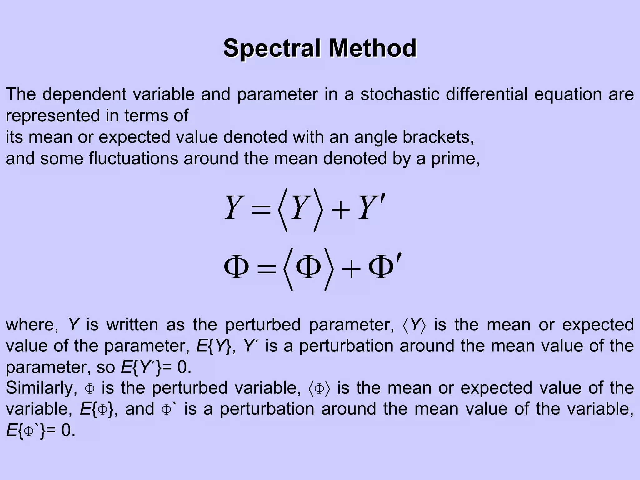
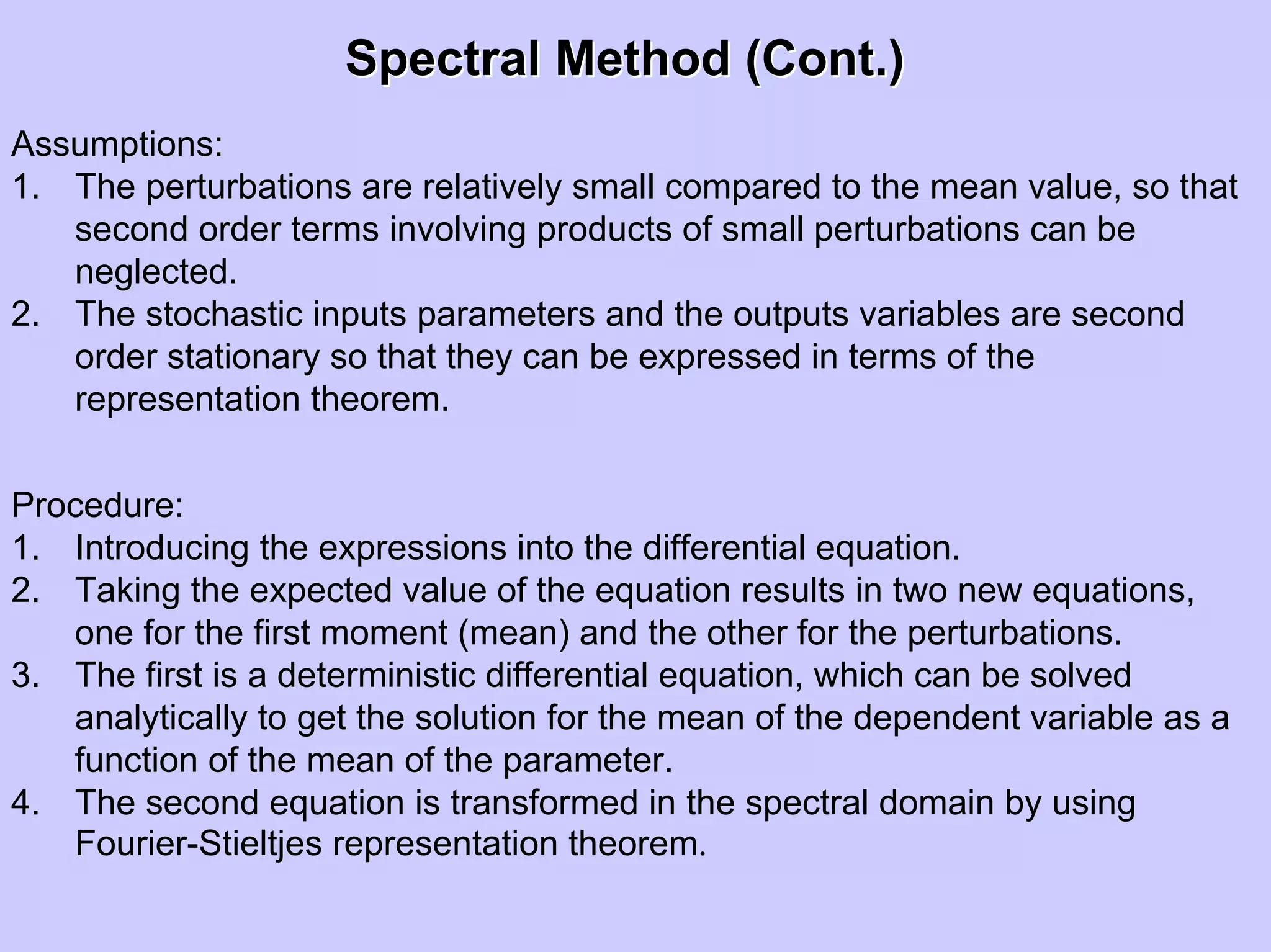
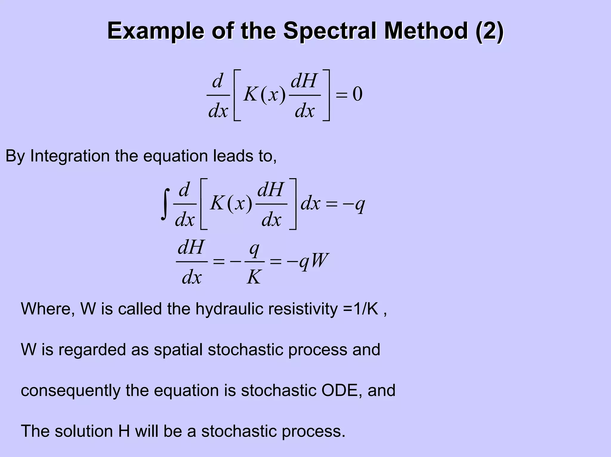
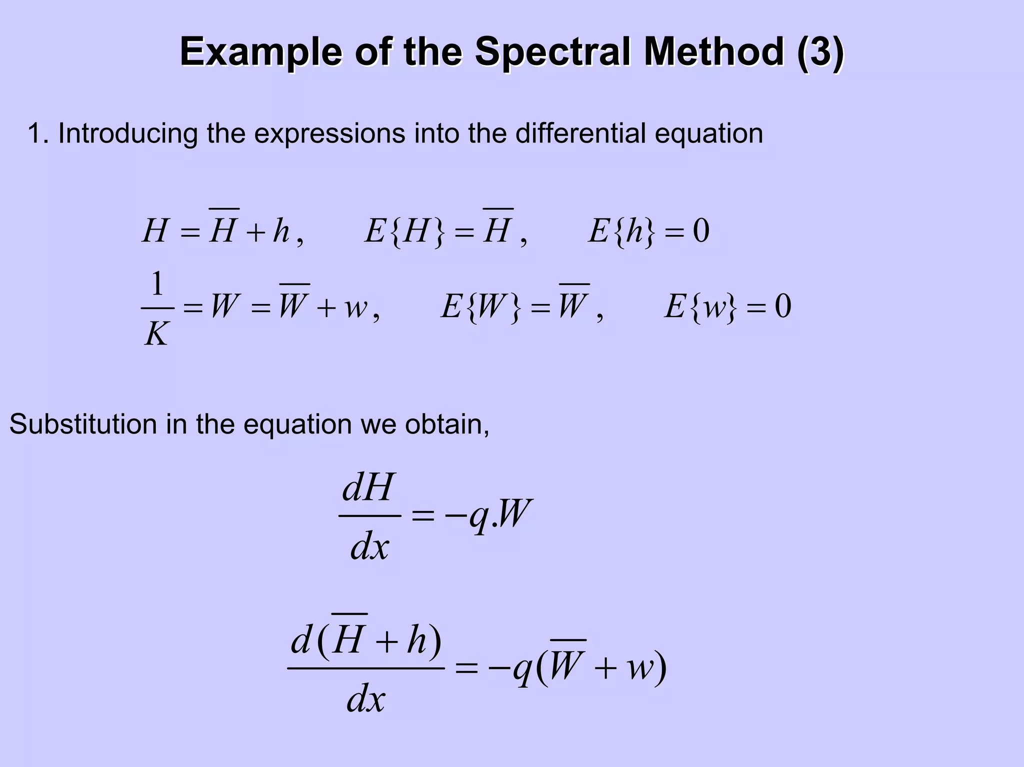
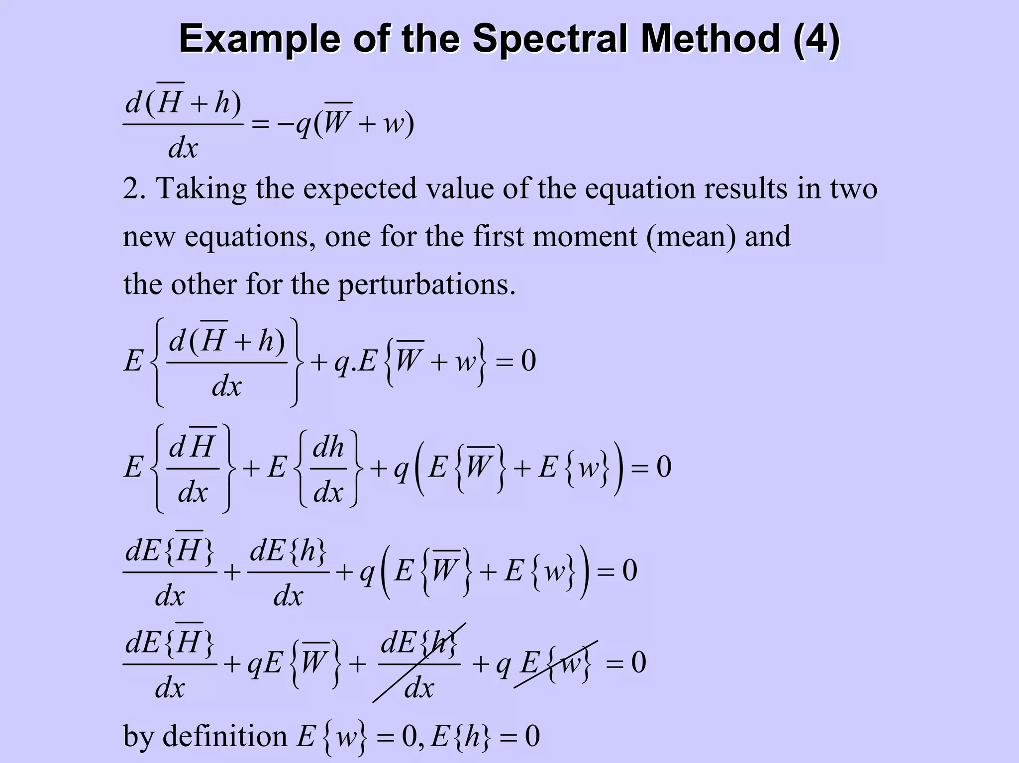
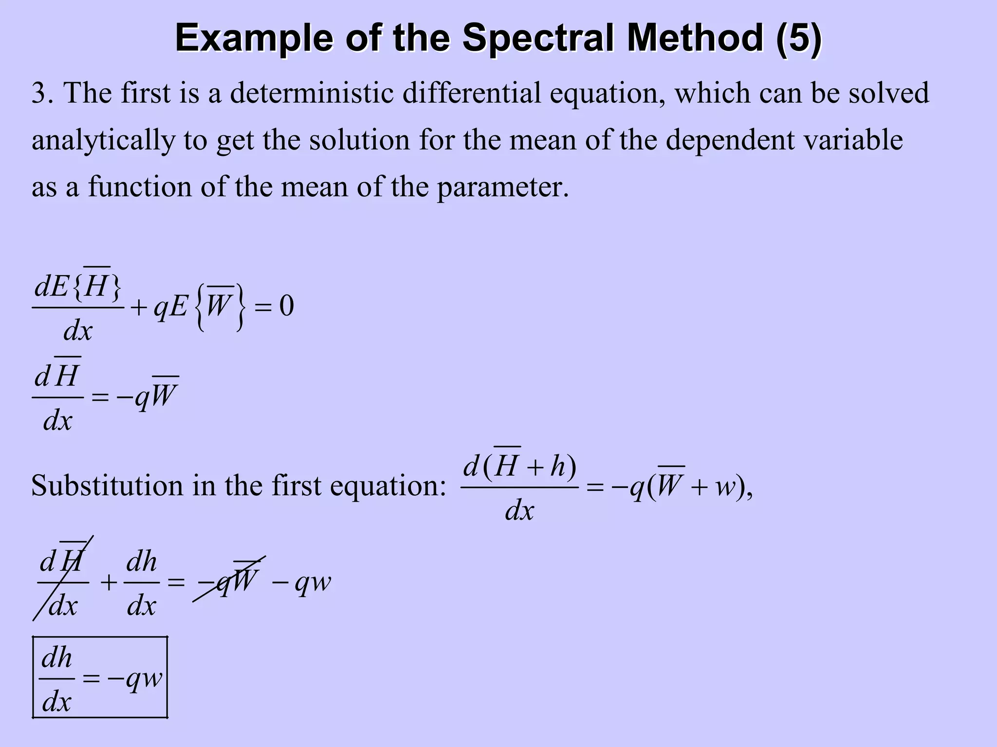
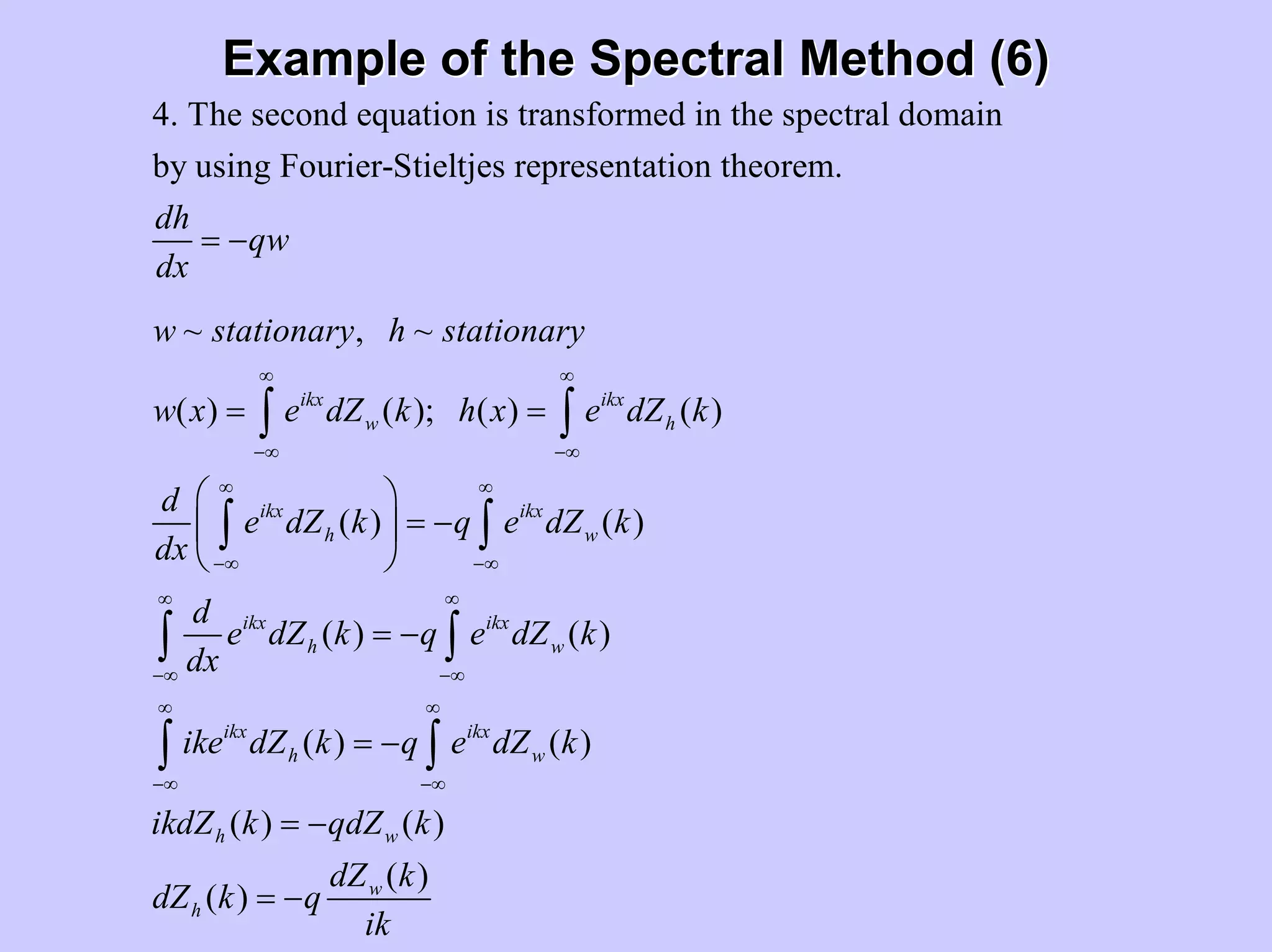
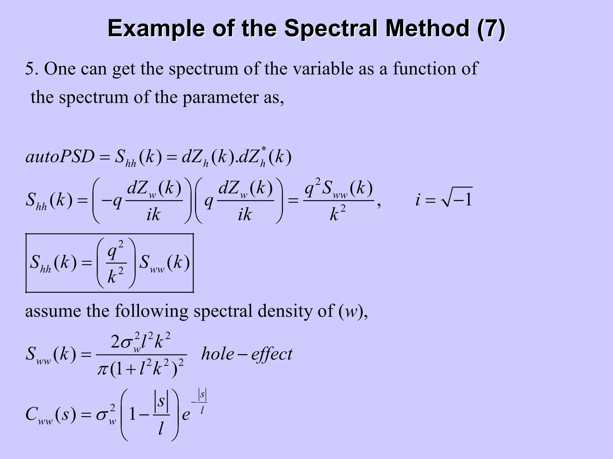
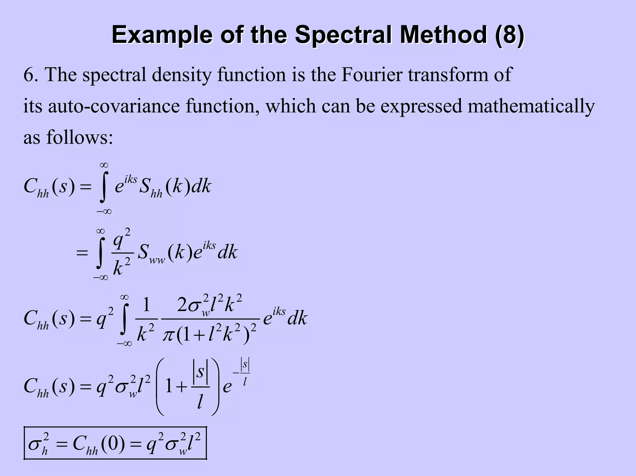
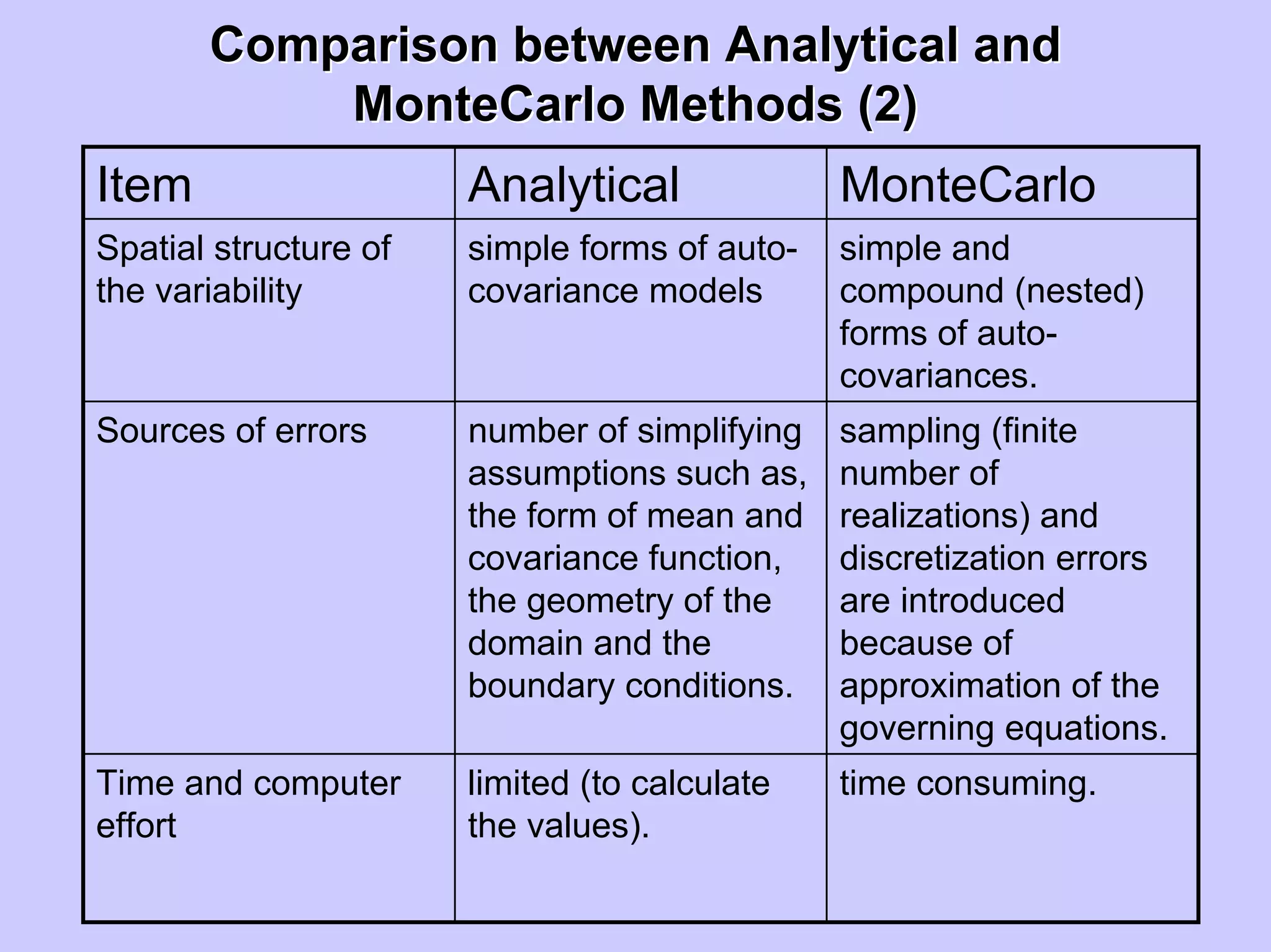
Stochastic differential equations (SDEs) describe systems with random components. Common methods to solve SDEs include spectral and perturbation methods. The spectral method represents variables and parameters as mean values plus fluctuations. Taking the expected value of the SDE yields equations for the mean and fluctuations that can be solved. The perturbation method expresses variables and parameters as power series expansions. Introducing these into the SDE allows analytical or numerical solution. SDEs are used to model systems with uncertain parameters like groundwater flow with random hydraulic conductivity.
![Analytical Solution in 2D Unbounded FlowAnalytical Solution in 2D Unbounded Flow
FieldField
( )
2 2
2
3/ 22 2
2 2 2 2
2 2 2
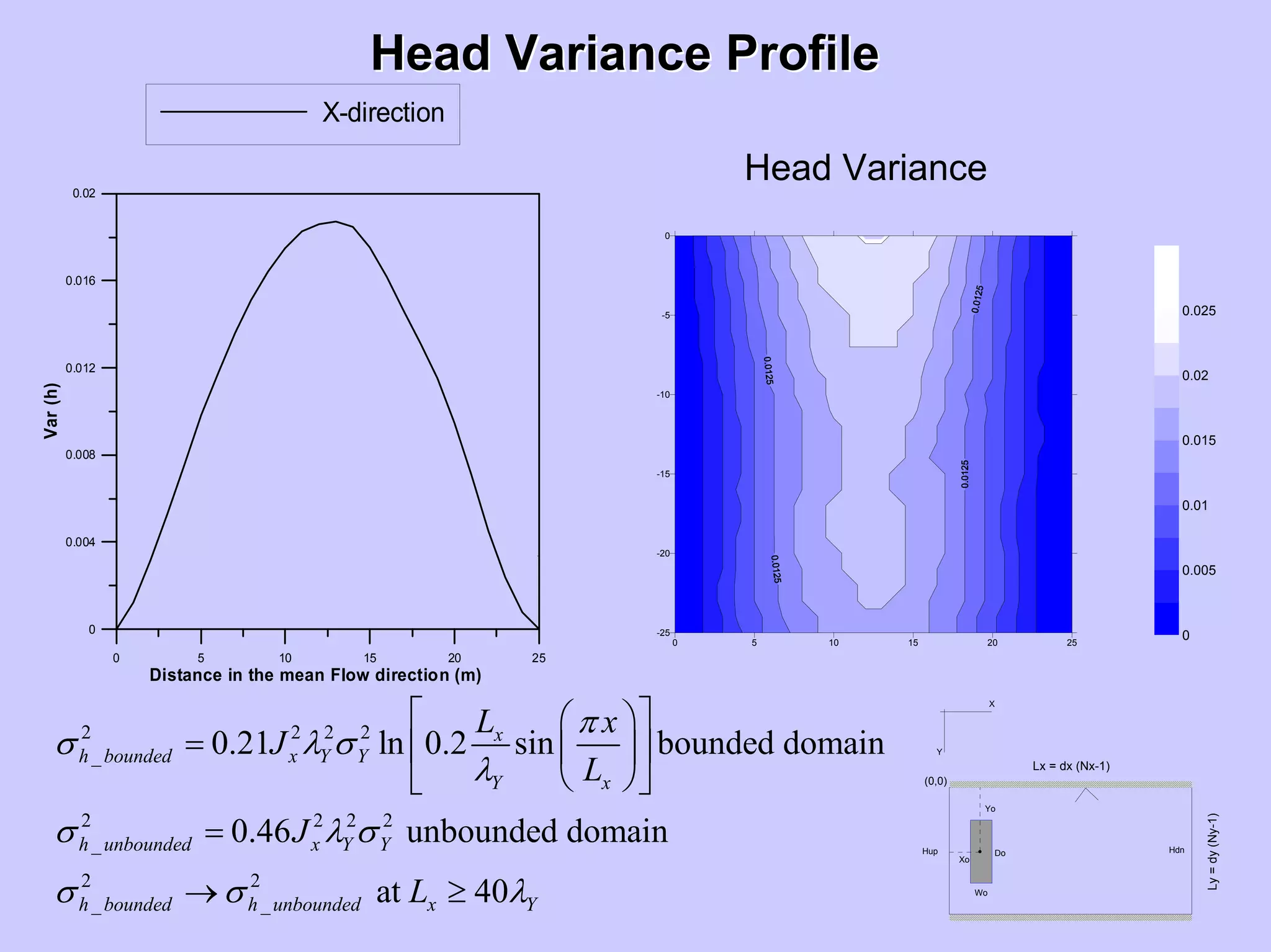
In 2D flow domain with exponential isotropic
covariance of Y=ln (K) given by,
( ) , ( )
2 1
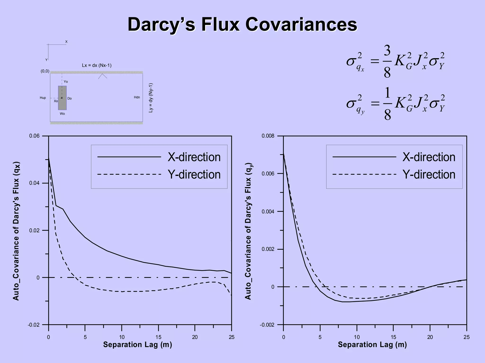
The perturbation solution is given by Dagan [1989],
0.46
3
8
Y
x
Y Y
YY Y YY
Y
h x Y Y
q G x
C e S
J
K J
λ σ λ
σ
π λ
σ λ σ
σ σ
−
= =
+
=
=
s
s k
k
2
2 2 2 2
1
2
1
8
( ) cos( ) 1 1
y
Y
Y
q G x Y
Yh Y x Y
Y Y
K J
C J e
λ
σ σ
σ λ χ
λ λ
⎛ ⎞ −
−⎜ ⎟⎜ ⎟
⎝ ⎠
=
⎧ ⎫⎡ ⎤⎛ ⎞ ⎛ ⎞⎪ ⎪
= + −⎨ ⎬⎢ ⎥⎜ ⎟ ⎜ ⎟
⎝ ⎠ ⎝ ⎠⎣ ⎦⎪ ⎪⎩ ⎭
s
s s
s](https://image.slidesharecdn.com/lecture5-190408192109/75/Lecture-5-Stochastic-Hydrology-17-2048.jpg)
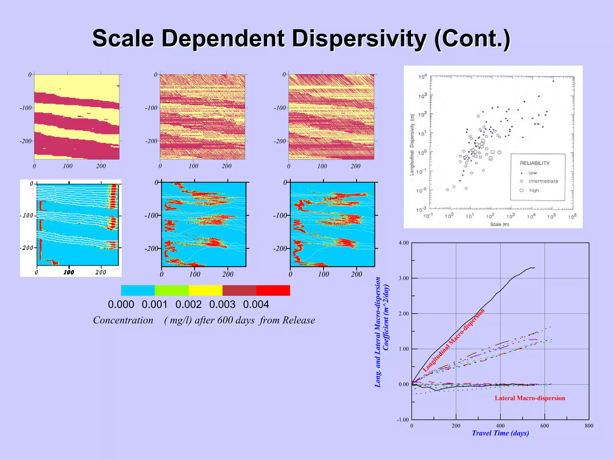
![ScaleScale--DependentDependent DispersivityDispersivity
Field Longitudinal Dispersivity Data Classified According to Reliability
[after Gelhar, et al., 1992],](https://image.slidesharecdn.com/lecture5-190408192109/75/Lecture-5-Stochastic-Hydrology-20-2048.jpg)
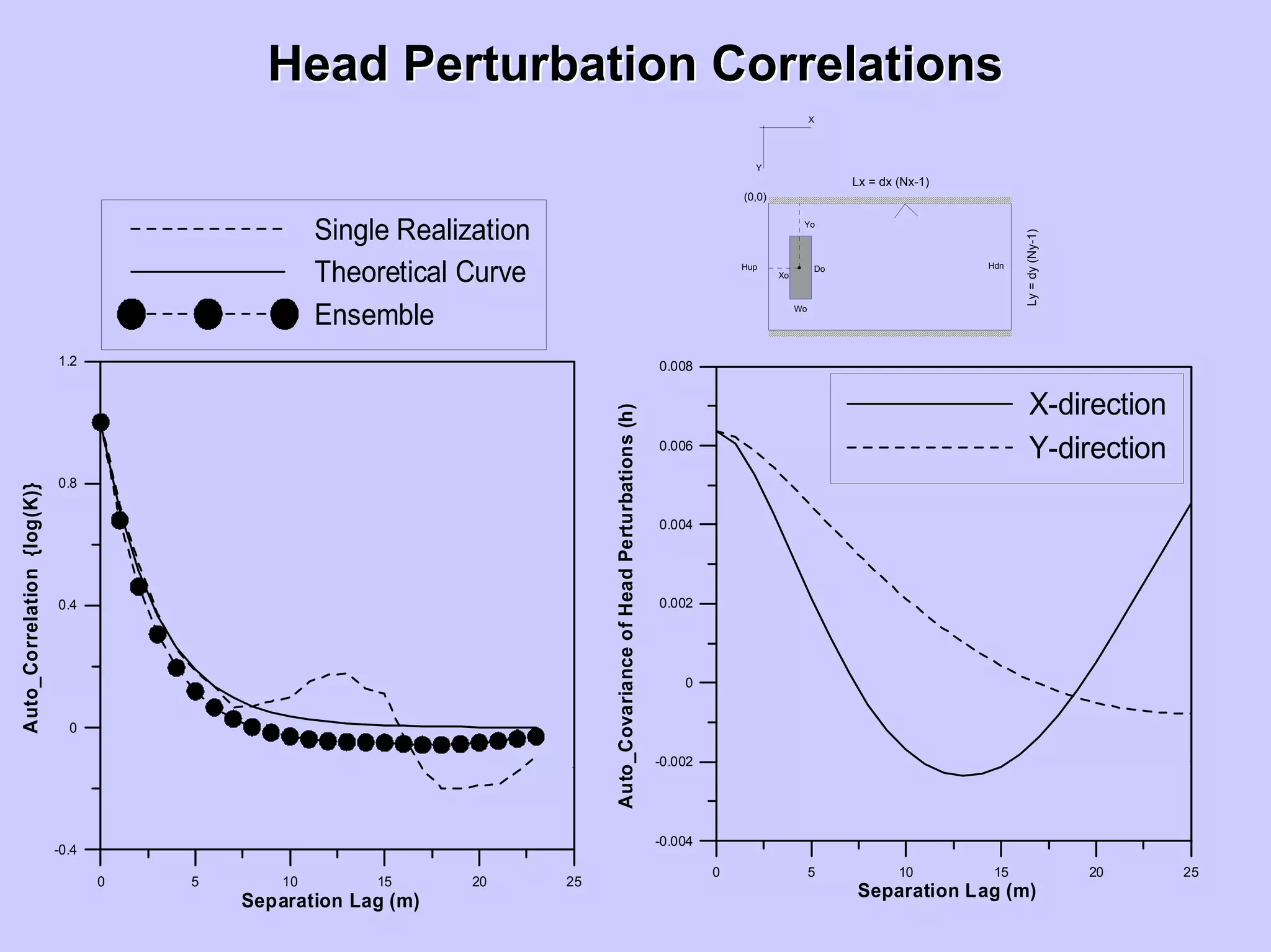
![HeadHead VariogramsVariograms
0 5 10 15 20 25
Separation Lag (m)
0
0.1
0.2
0.3
0.4
0.5
VariogramoftheHead(H)
X-direction
Y-direction
0 5 10 15 20 25
Separation Lag (m)
0
0.002
0.004
0.006
0.008
0.01
VariogramoftheHead(H)
Y-direction
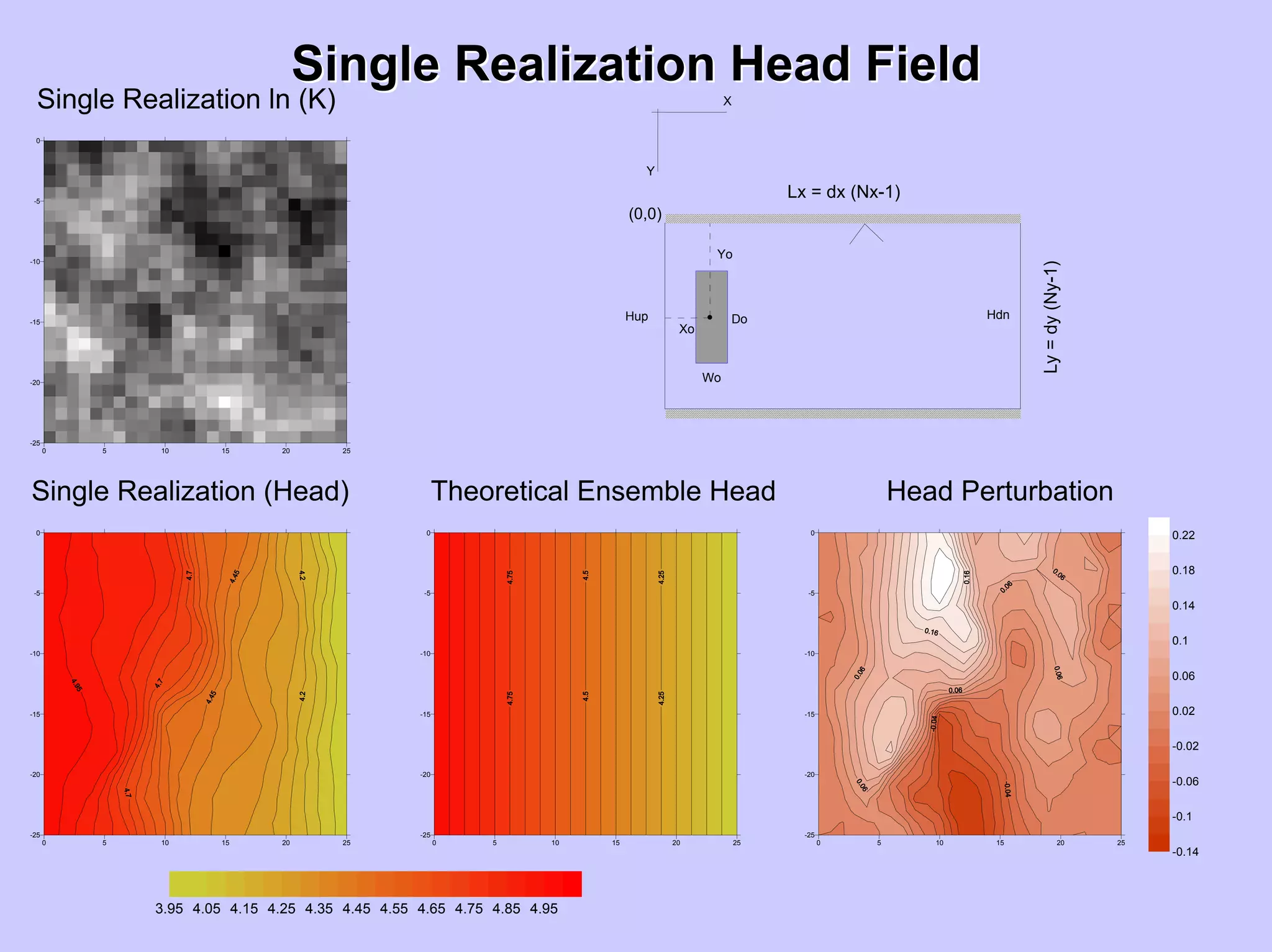
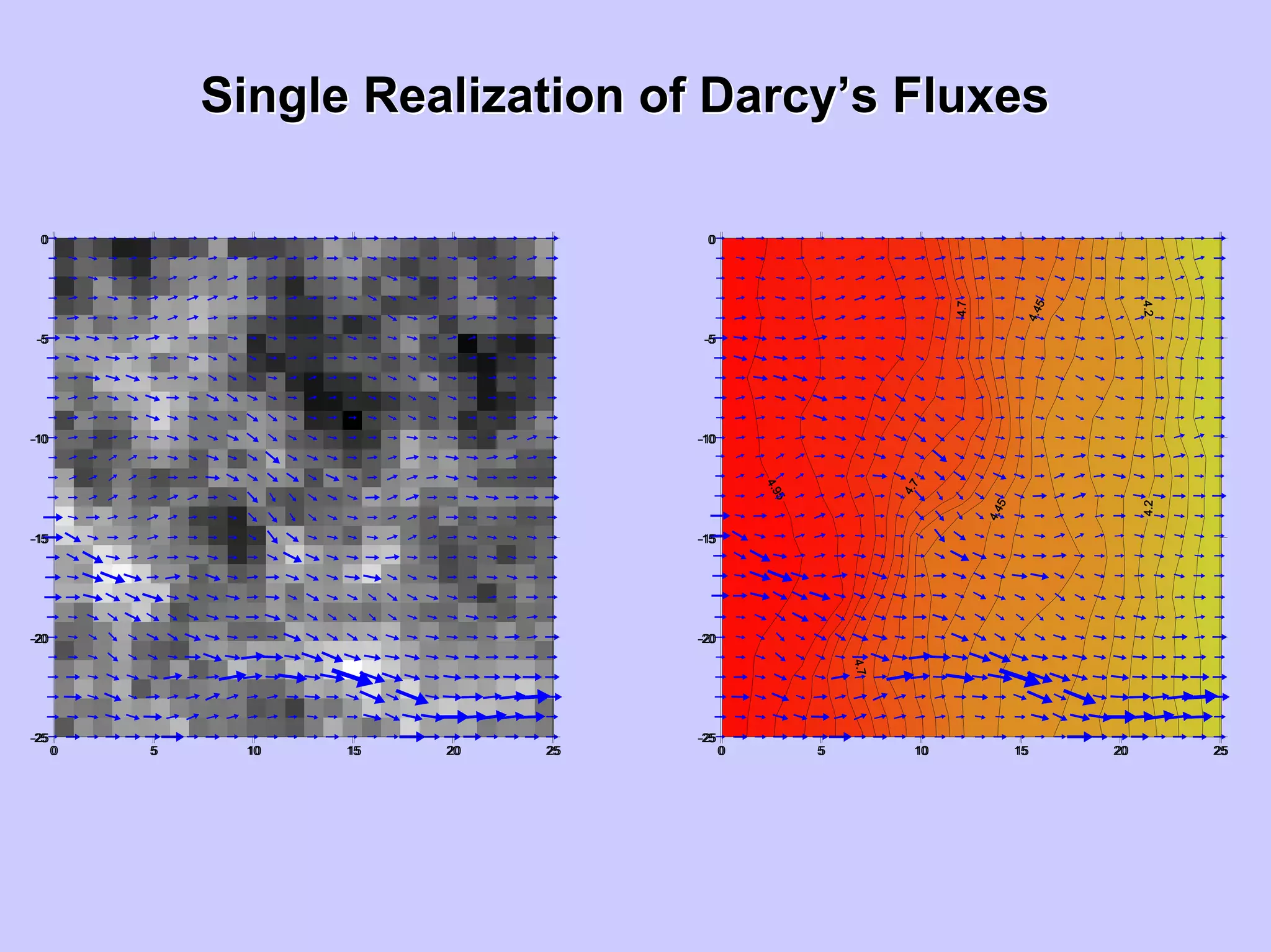
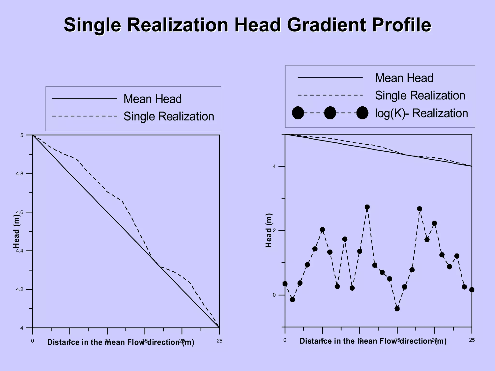
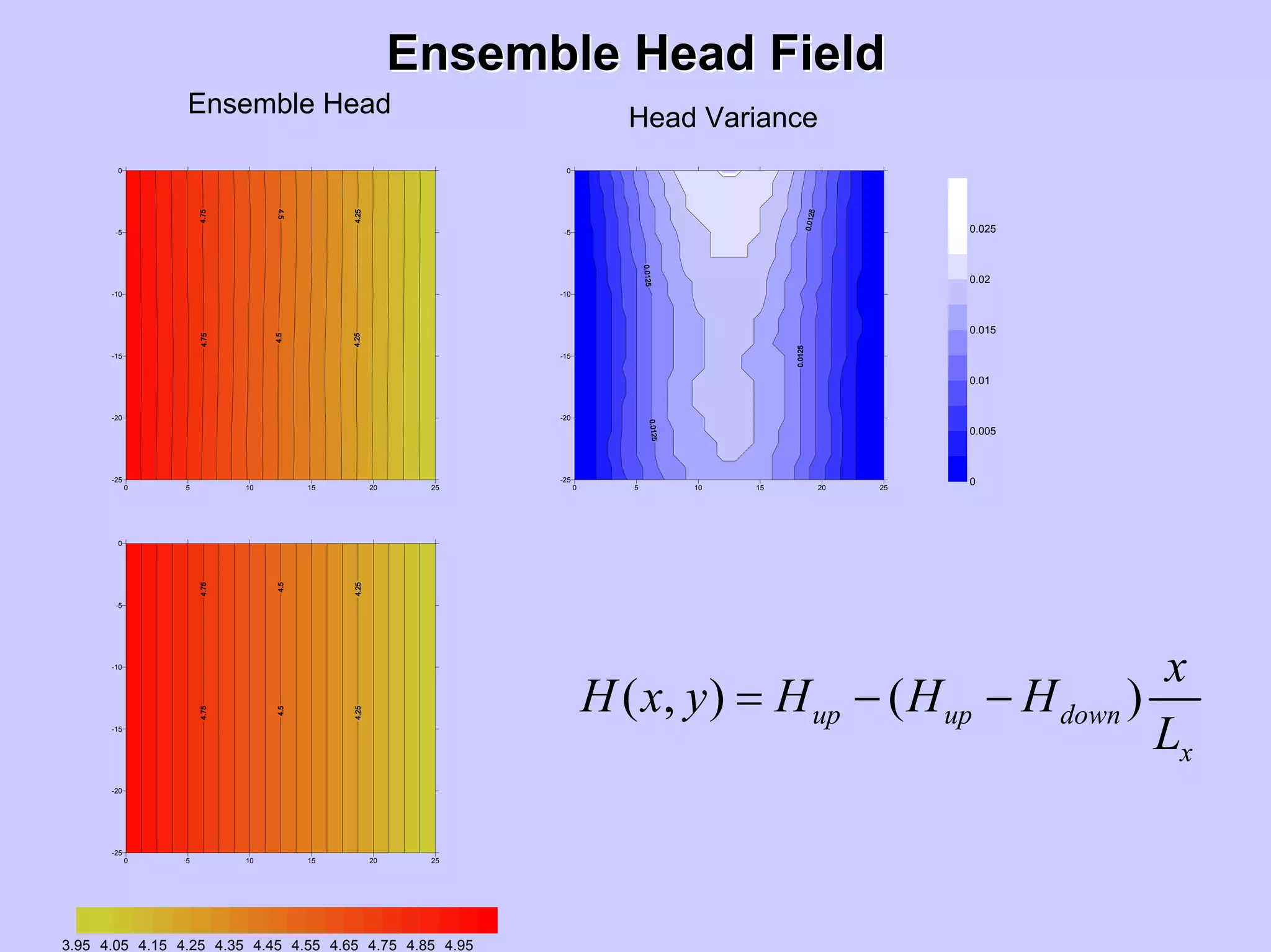
( , ) ( )up up down
x
x
H x y H H H
L
= − −
[ ]
( )
2
1
1
( ) ( )- ( )
2 ( )
n
i
Z Z
n
γ
=
= ∑
s
s x +s x
s ,
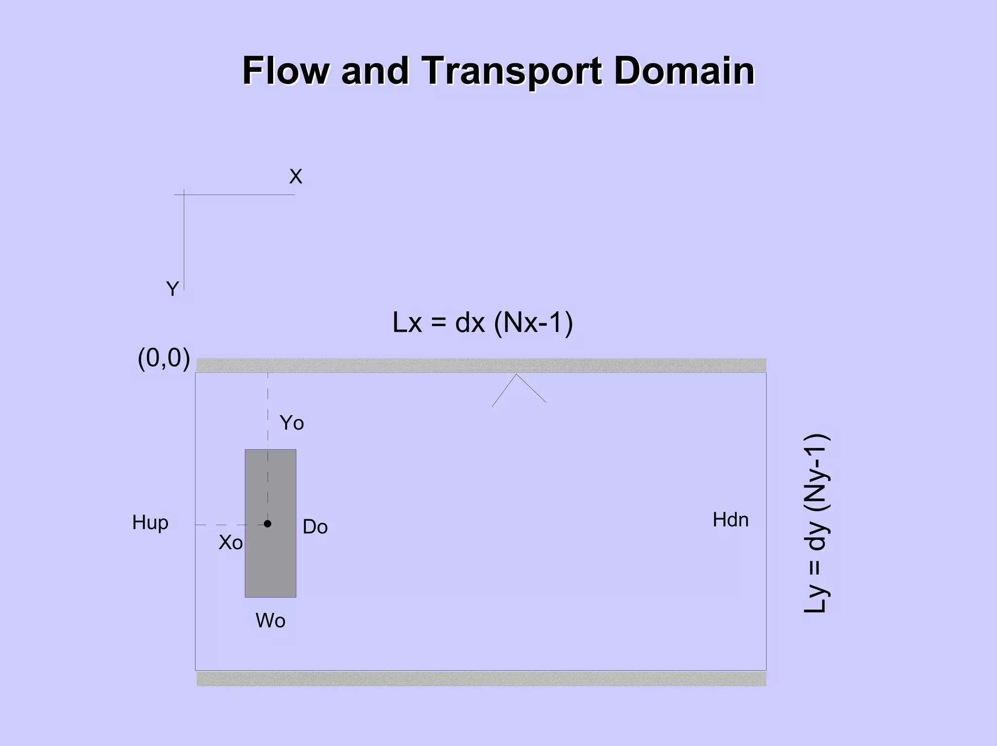
Lx = dx (Nx-1)
Ly=dy(Ny-1)
X
Y
(0,0)
Yo
Xo
Do
Wo
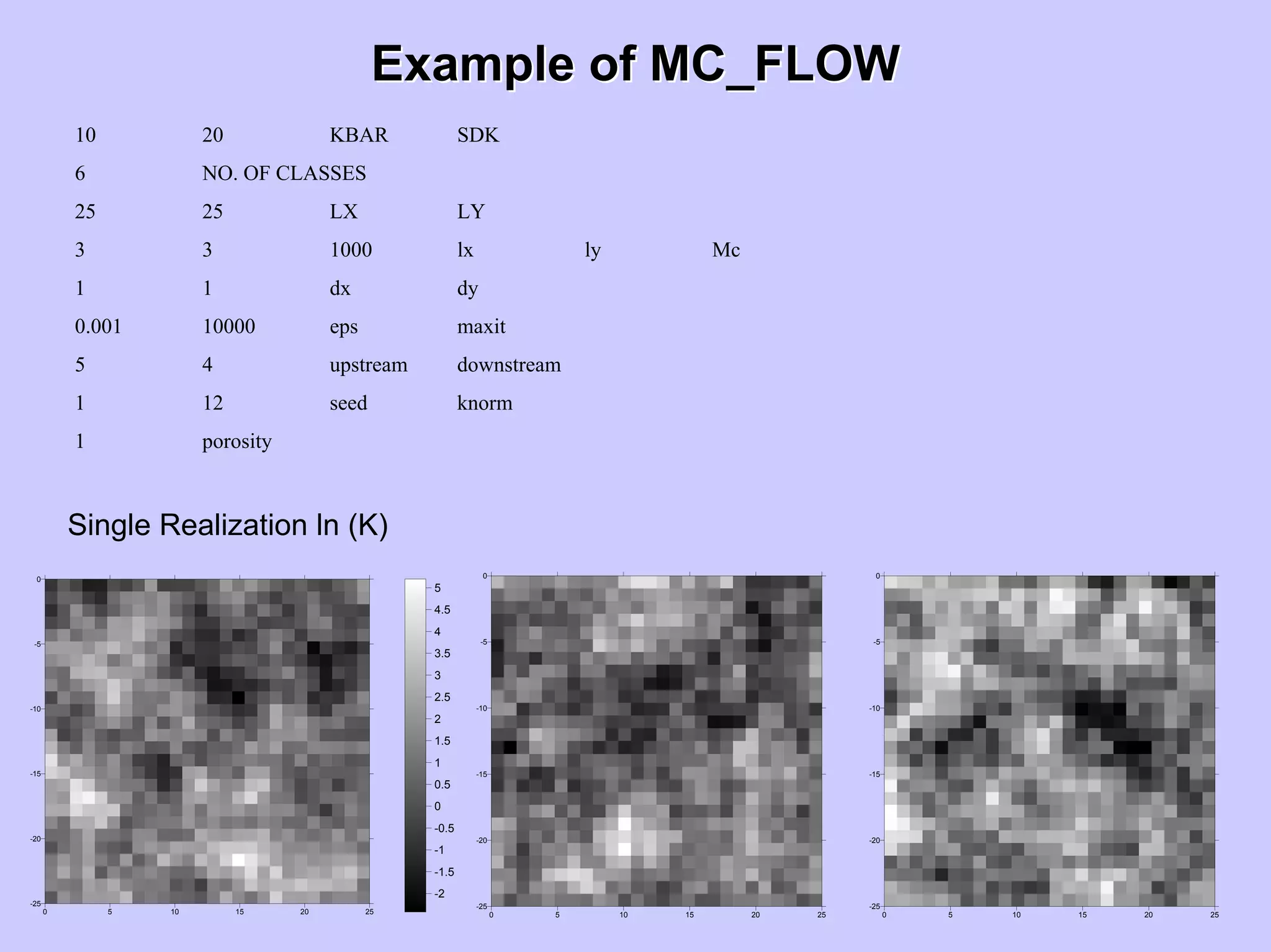
Hup Hdn](https://image.slidesharecdn.com/lecture5-190408192109/75/Lecture-5-Stochastic-Hydrology-31-2048.jpg)

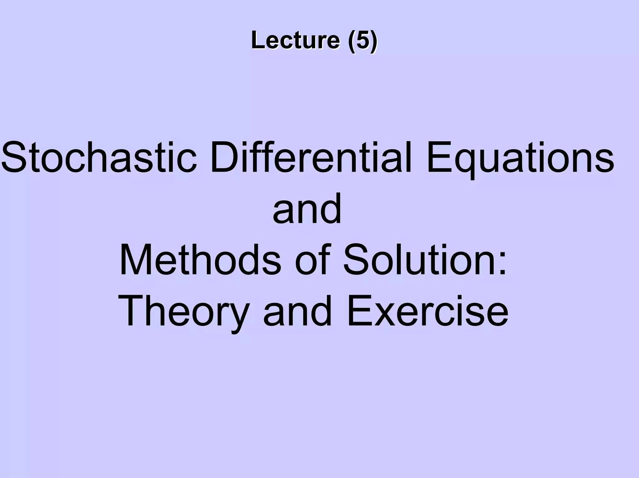
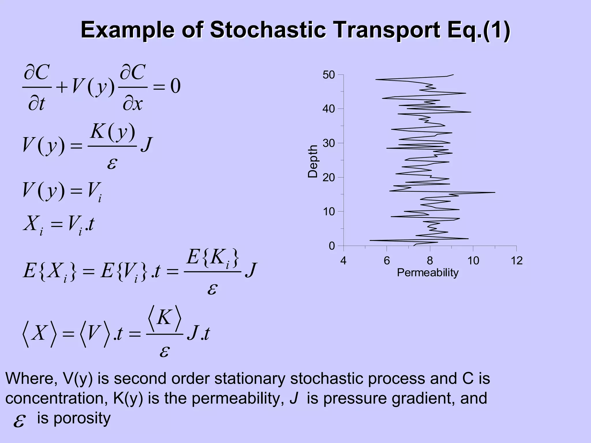
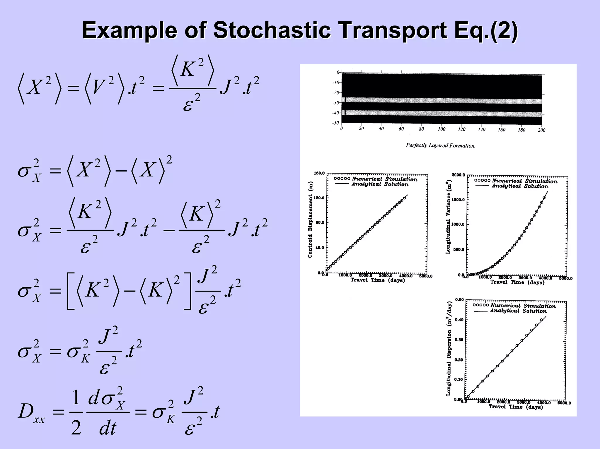
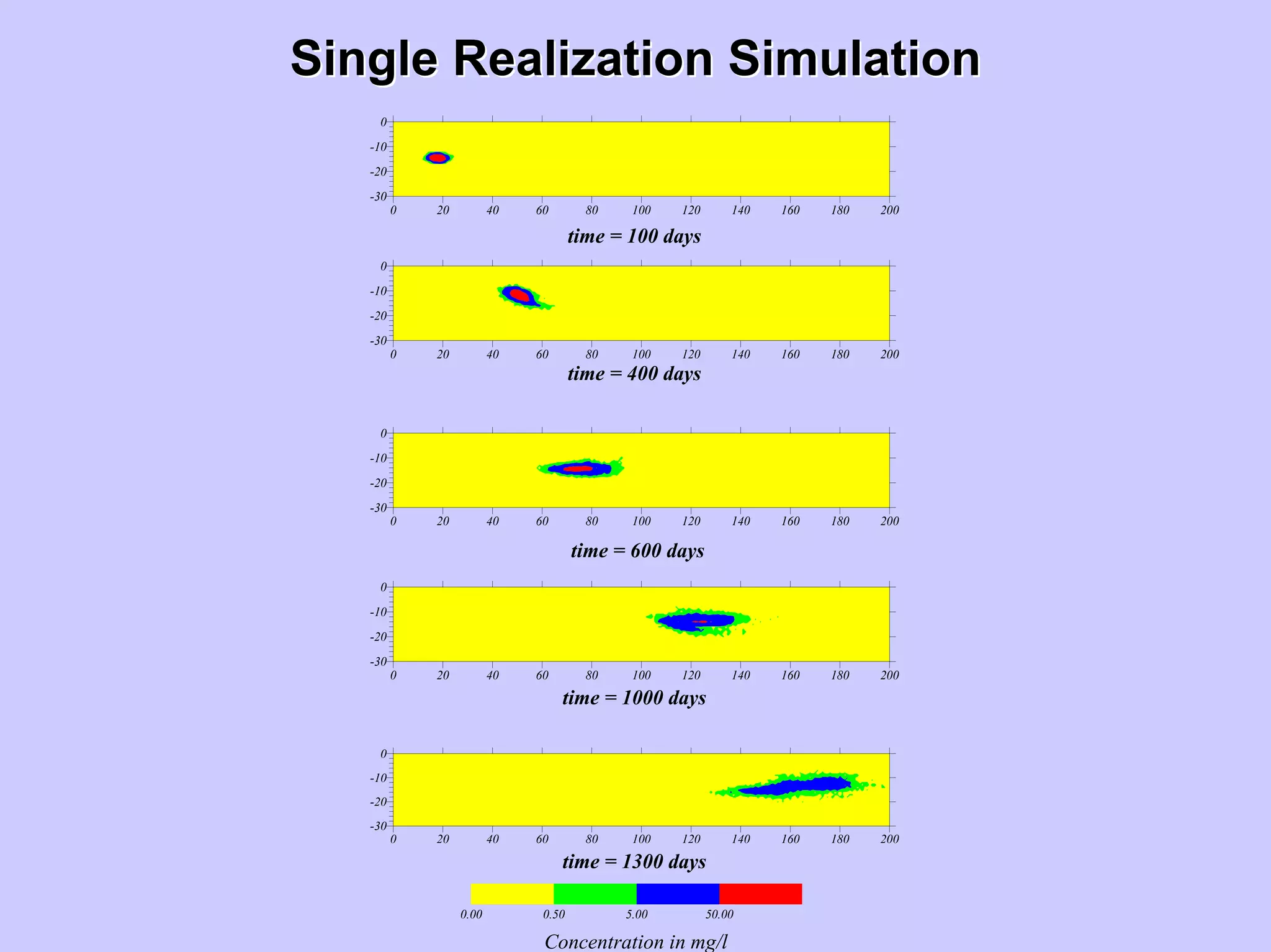
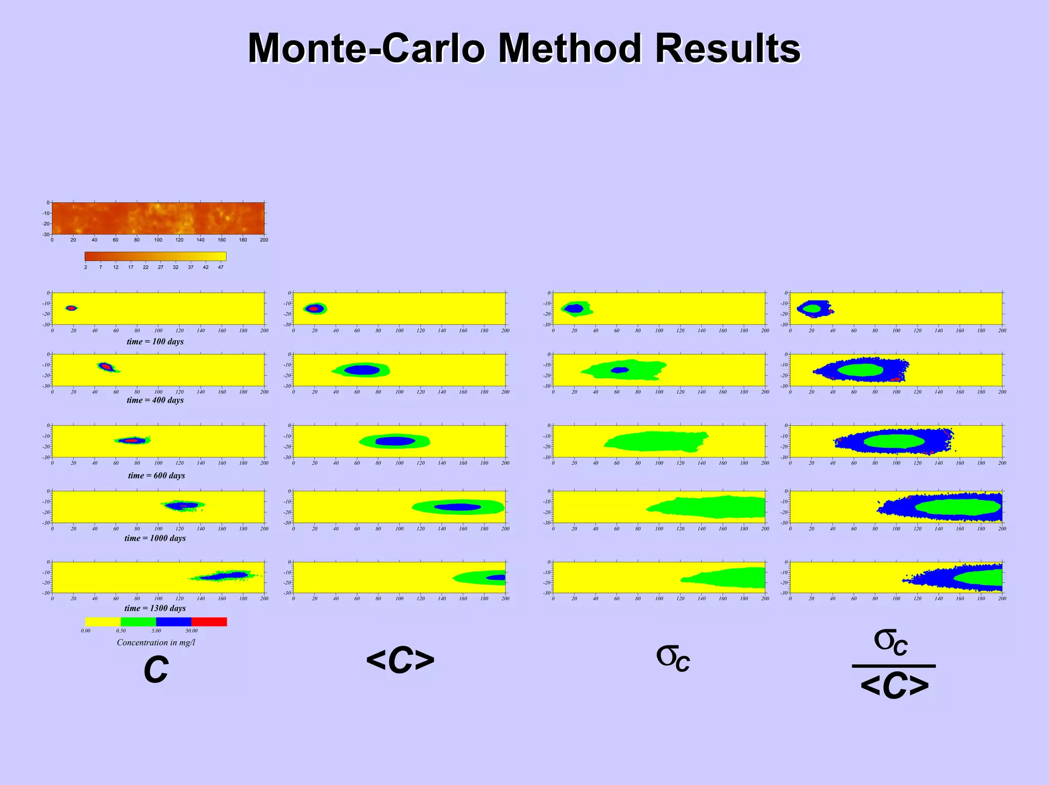
![Solute Transport EquationSolute Transport Equation
[ ] WCC
CQ
S
+CV
xx
C
D
xt
C
SinkSource
Decay
reactionChemicalAdvection
i
i
DiffusionDispersion
j
ij
i
/
)'(
ε
−
+λ−
ε∂
∂
−
⎥
⎥
⎦
⎤
⎢
⎢
⎣
⎡
∂
∂
∂
∂
=
∂
∂
−
−
where
C is the concentration field at time t,
S is solute concentration of species in the source or sink fluid,
i, j are counters,
C’ is the concentration of the dissolved solutes in a source or sink,
W is a general term for source or sink and
Vi is the component of the Eulerian interstitial velocity in xi direction
defined as follows,
Dij is the hydrodynamic dispersion tensor,
Q is the volumetric flow rate per unit volume of the source or sink,
j
ij
i
x
K
-=V
∂
Φ∂
ε
where
Kij is the hydraulic conductivity tensor, and ε is the porosity of the medium.](https://image.slidesharecdn.com/lecture5-190408192109/75/Lecture-5-Stochastic-Hydrology-36-2048.jpg)


![01-[Albert_Boggess,_Francis_J._Narcowich]_A_First_Cou(BookZZ.org).pdf](https://cdn.slidesharecdn.com/ss_thumbnails/01-albertboggessfrancisj-220602130045-9a8f9563-thumbnail.jpg?width=640&height=640&fit=bounds)