An image histogram represents the distribution of pixel intensities in a digital image. It plots the number of pixels for each tonal value. Histograms can reveal if an image is under-exposed or over-exposed based on where most pixel values are concentrated. Histogram equalization improves contrast by spreading out pixel values across intensity levels. Local histogram equalization applies this within neighborhoods to enhance detail while preserving edges.

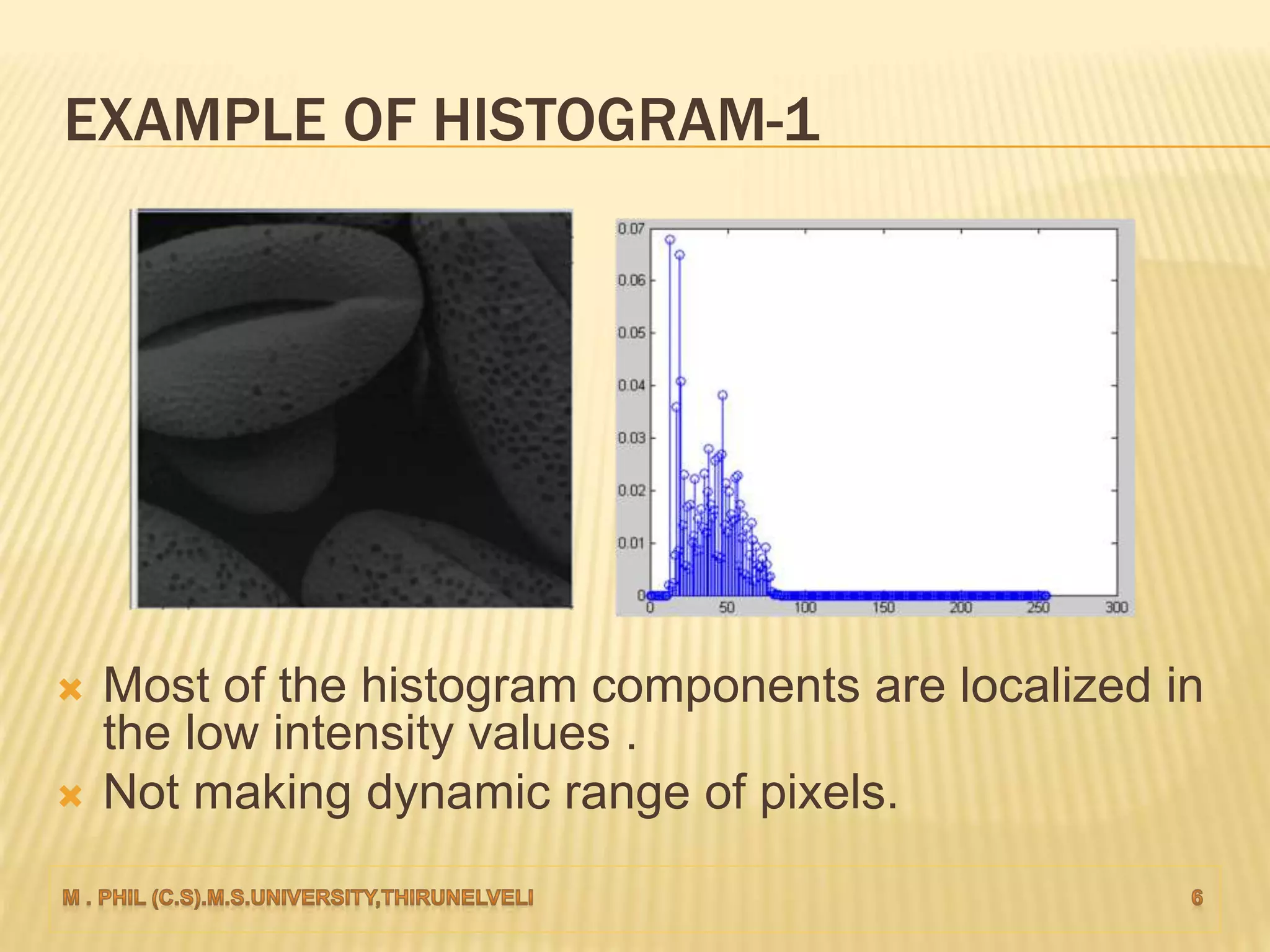
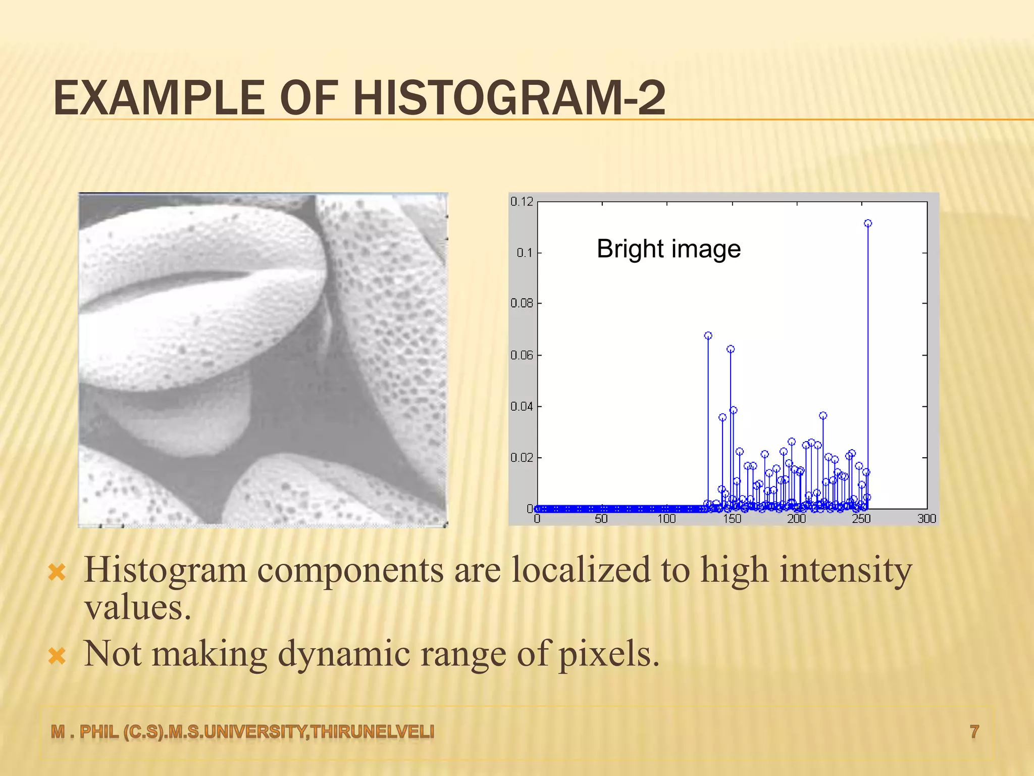
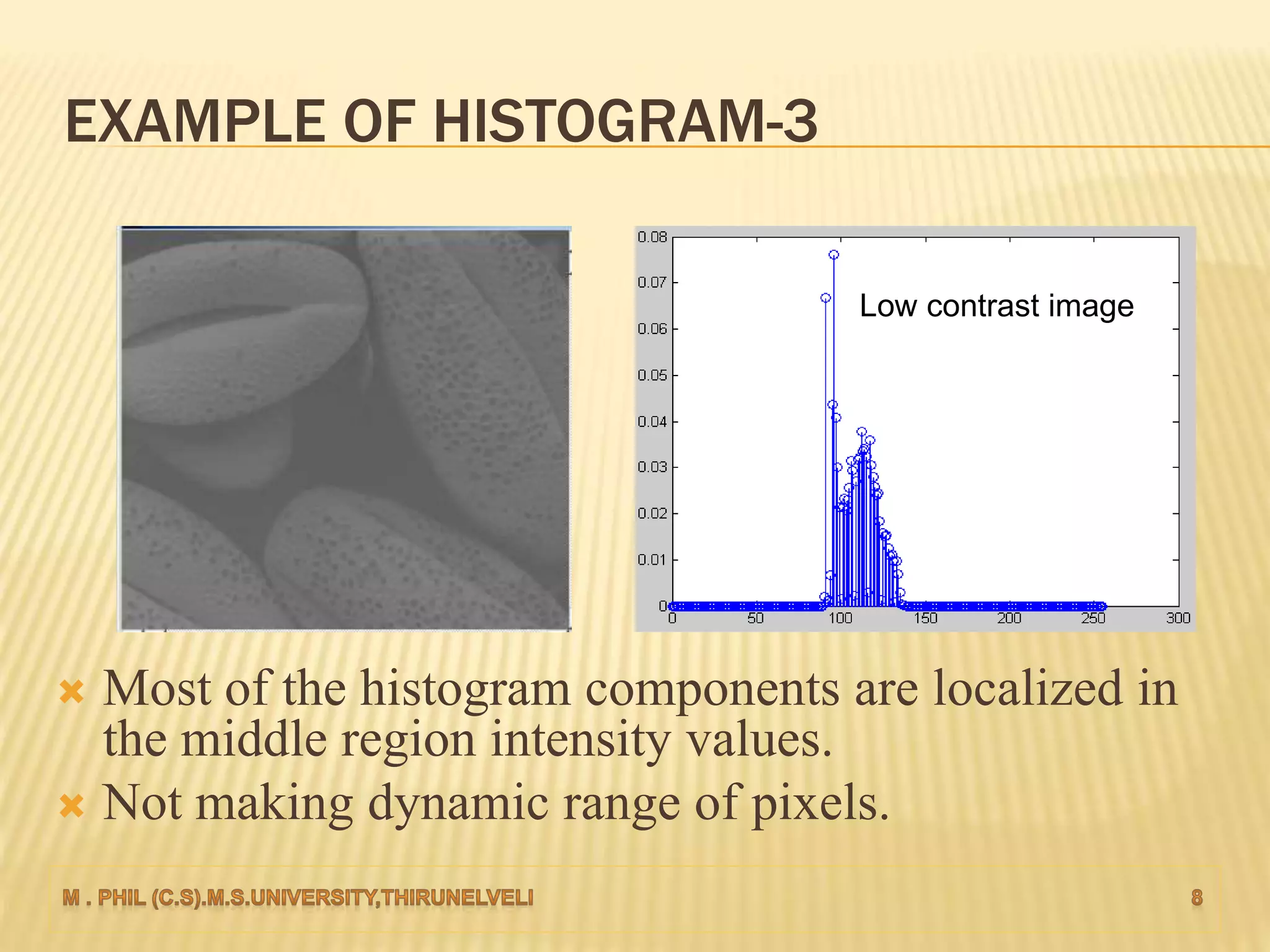
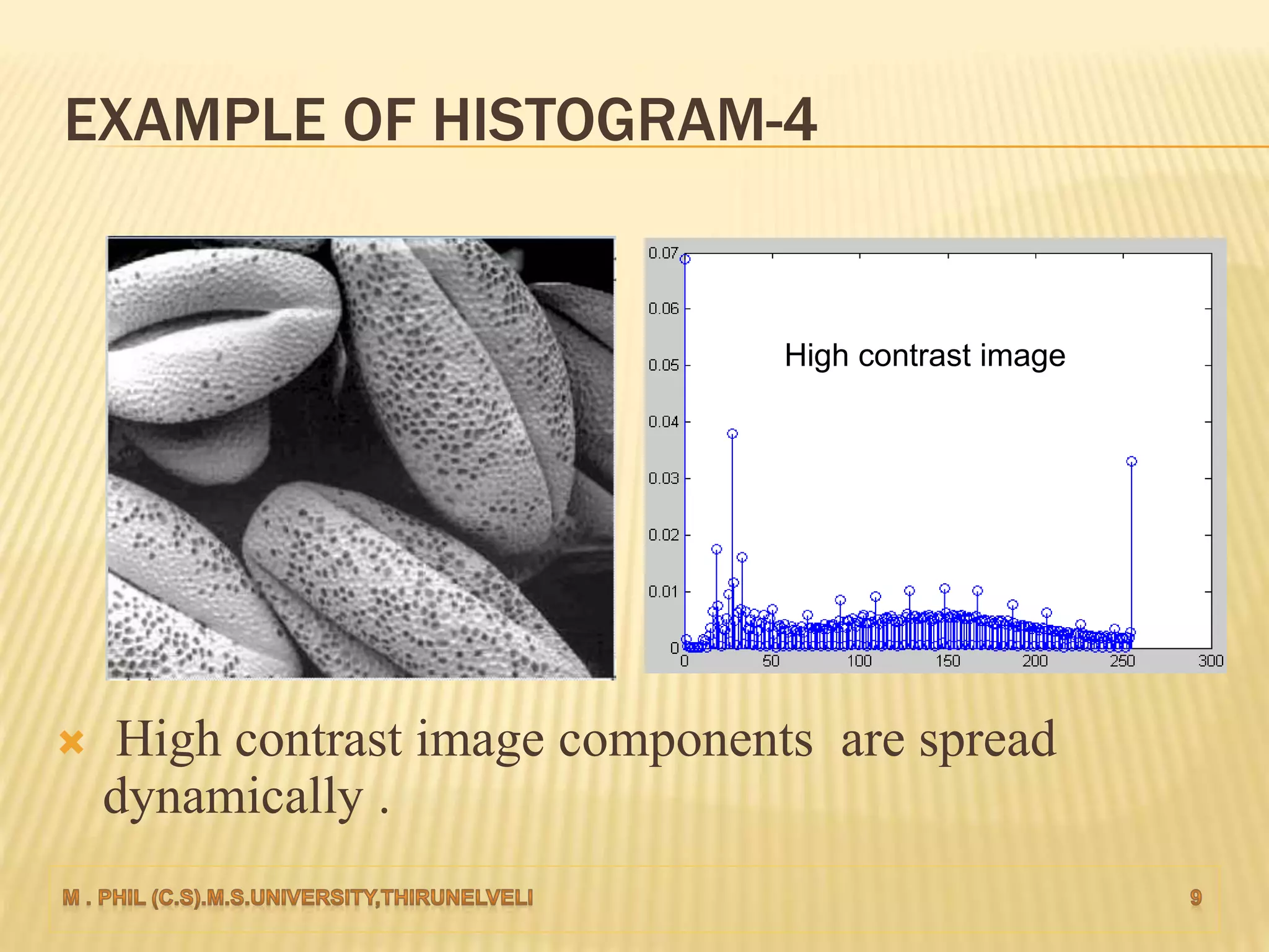
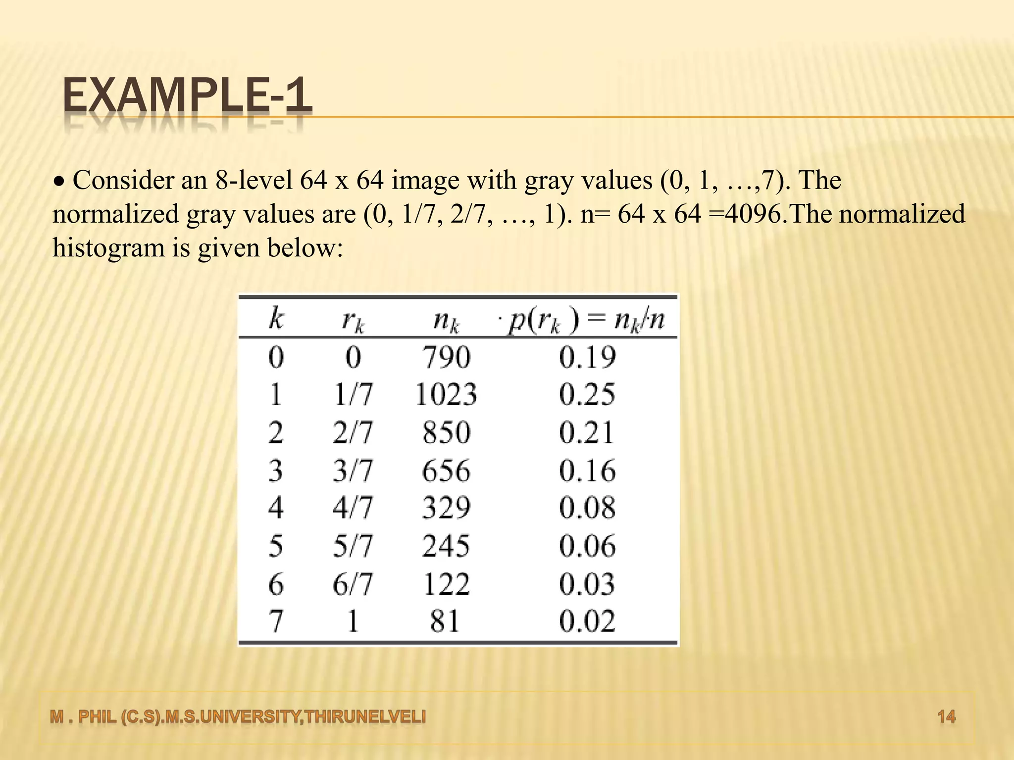
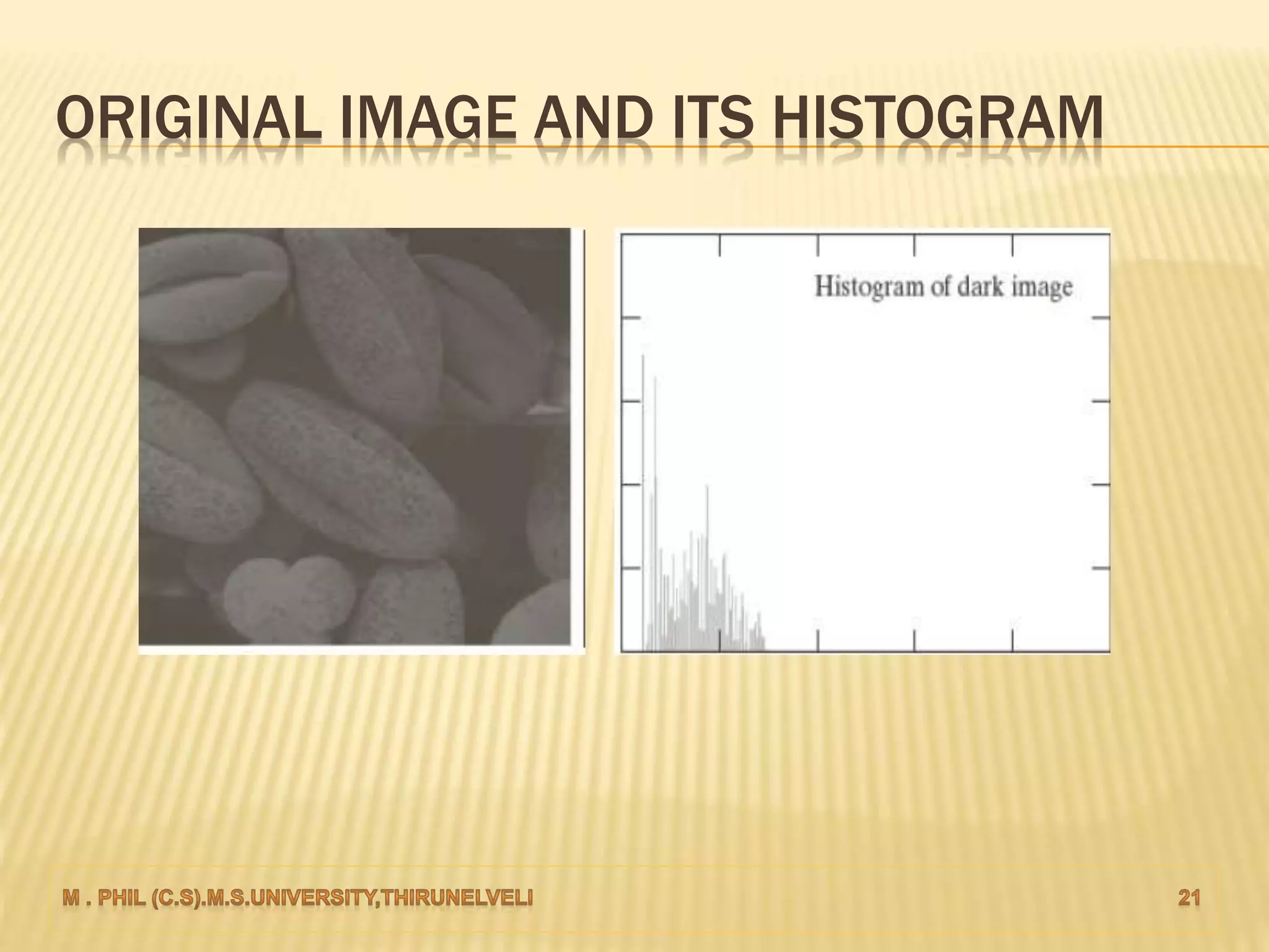
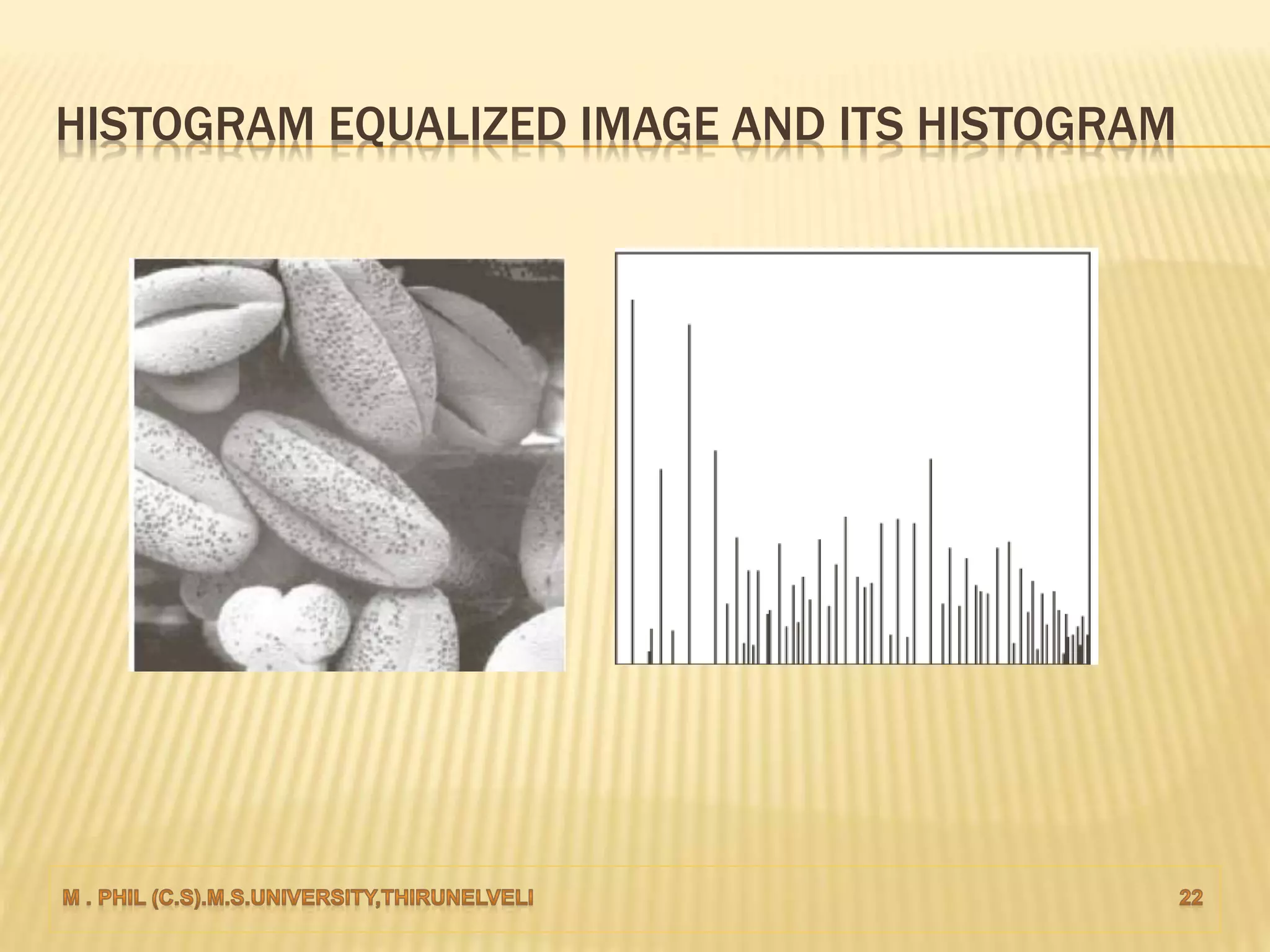
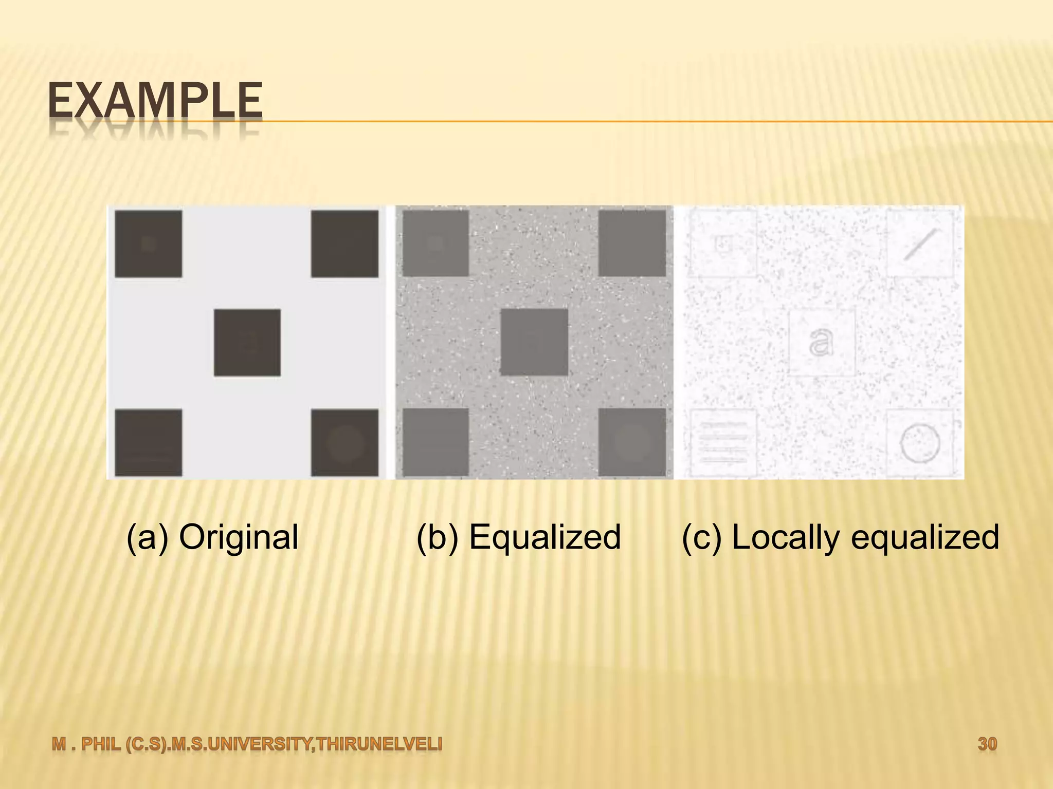
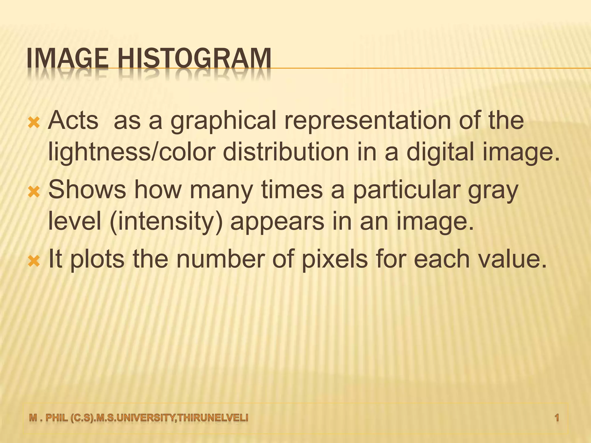
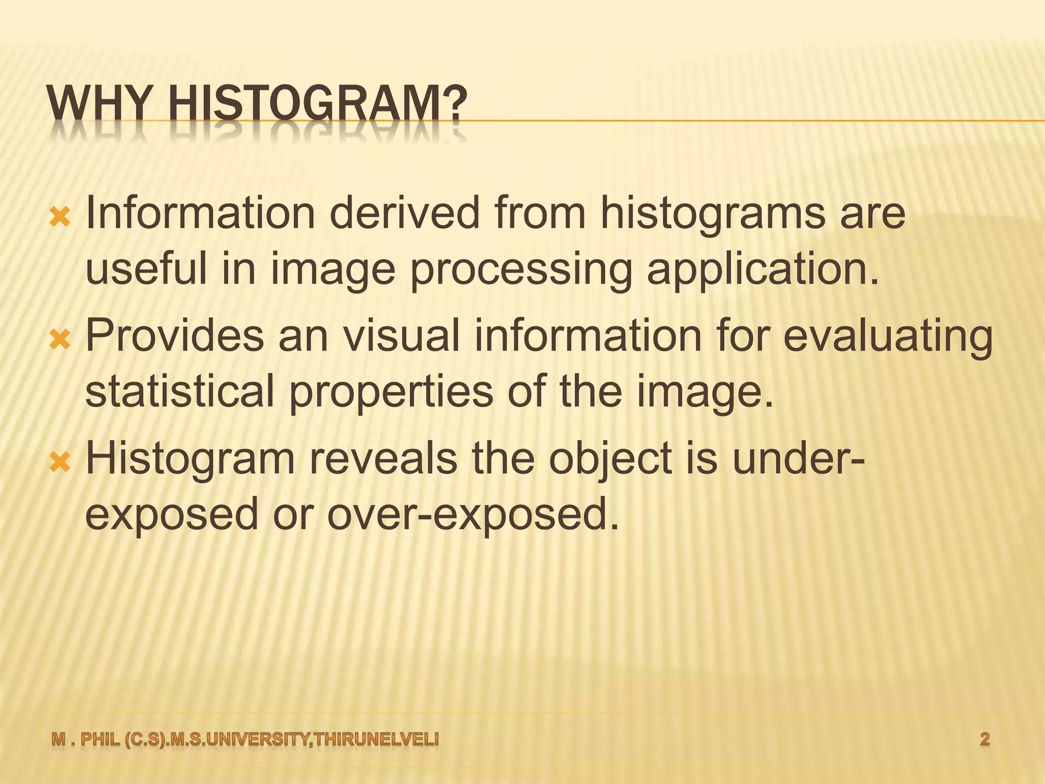
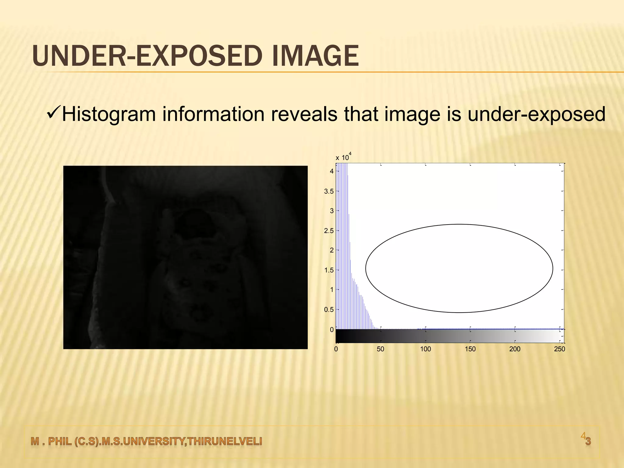
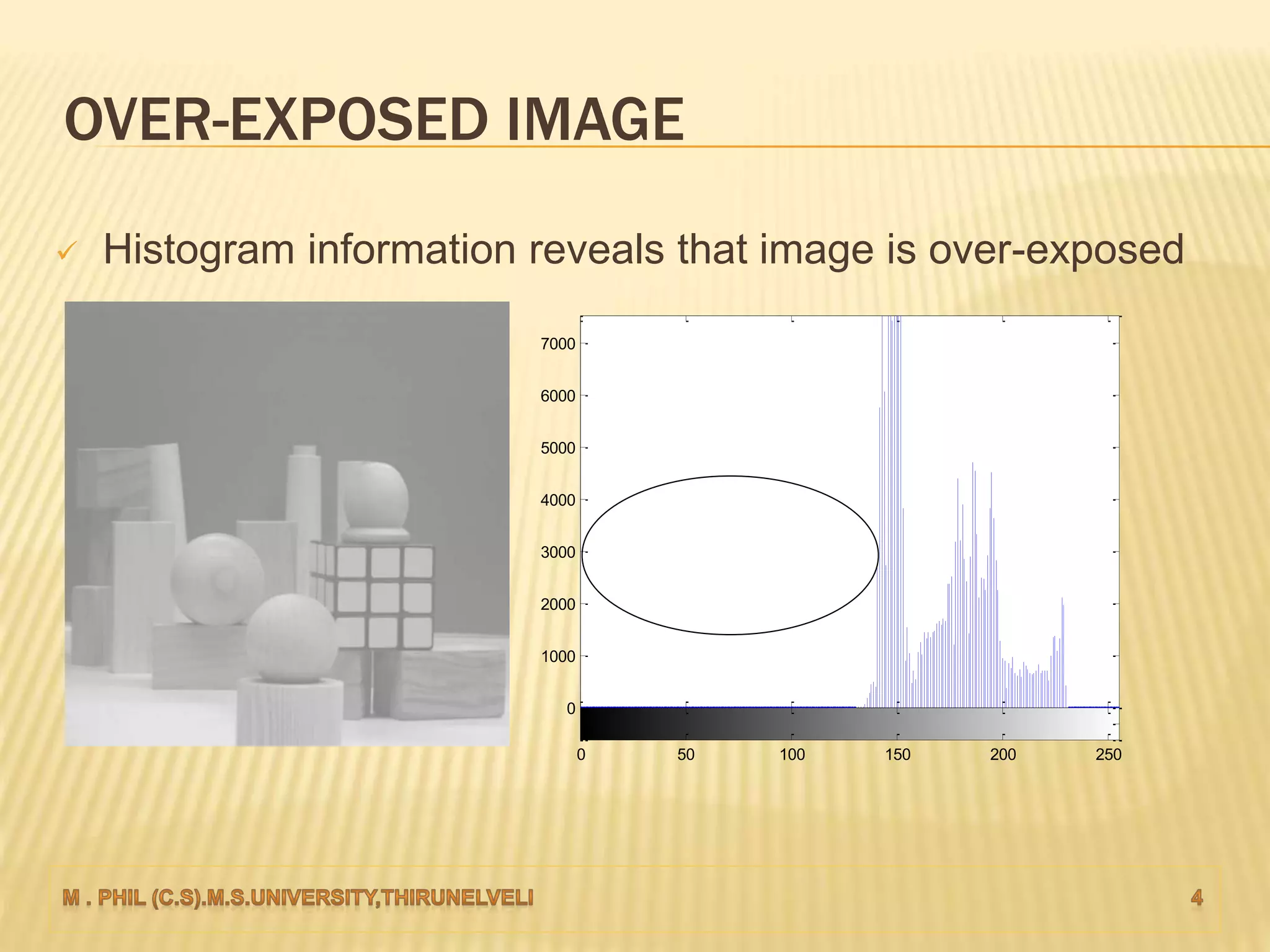
2. IMAGE HISTOGRAM
 Acts as a graphical representation of the
lightness/color distribution in a digital image.
 Shows how many times a particular gray
level (intensity) appears in an image.
 It plots the number of pixels for each value.

3. WHY HISTOGRAM?
 Information derived from histograms are
useful in image processing application.
 Provides an visual information for evaluating
statistical properties of the image.
 Histogram reveals the object is under-
exposed or over-exposed.

4. 4
UNDER-EXPOSED IMAGE
0 50 100 150 200 250
0
0.5
1
1.5
2
2.5
3
3.5
4
x 10
4
Histogram information reveals that image is under-exposed

5. OVER-EXPOSED IMAGE
0 50 100 150 200 250
0
1000
2000
3000
4000
5000
6000
7000
 Histogram information reveals that image is over-exposed

6. HISTOGRAM PROCESSING
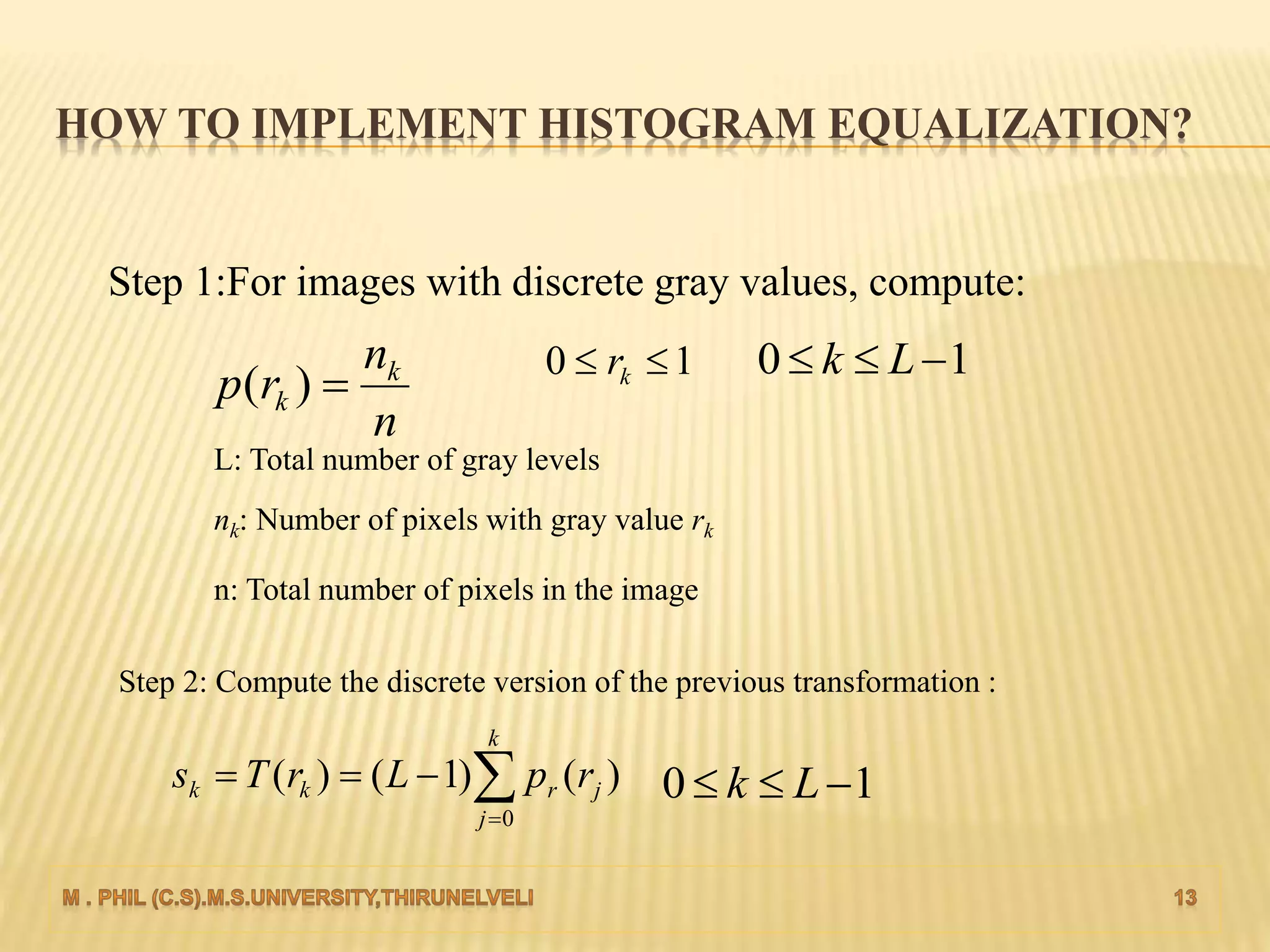
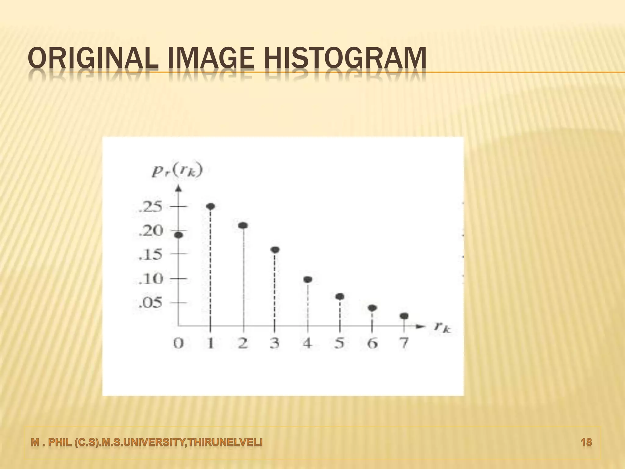
 The histogram of a digital image with gray
levels in the range [0, L-1]
 Discrete function:
h(rk) = nk
rk - kth gray level
nk - number of pixels in the image having
gray level rk.

7.  Most of the histogram components are localized in
the low intensity values .
 Not making dynamic range of pixels.
EXAMPLE OF HISTOGRAM-1

8.  Histogram components are localized to high intensity
values.
 Not making dynamic range of pixels.
EXAMPLE OF HISTOGRAM-2
Bright image

9.  Most of the histogram components are localized in
the middle region intensity values.
 Not making dynamic range of pixels.
EXAMPLE OF HISTOGRAM-3
Low contrast image

10.  High contrast image components are spread
dynamically .
EXAMPLE OF HISTOGRAM-4
High contrast image

11. EXAMPLE OF HISTOGRAM-4
 In histogram-4 components are distributed over
all the intensity range.
 Distribution is almost uniform with few peaks.
 If the distribution is uniform , the image tends to
have a high dynamic range and the details are
more easily perceived.
 Proved that high contrast image gives better
visual appearance.

12. HISTOGRAM PROCESSING
 Histogram Equalization
 Histogram Matching/Specification
 Local Histogram Processing

13. HISTOGRAM EQUALIZATION
 Techniques for adjusting image intensities to
enhance contrast.
 Used to improve the visual appearance of an
image.
 Spread out the frequencies in an image (or
equalizing image) is a simple way to dark or
washed out images.

14. HOW TO IMPLEMENT HISTOGRAM EQUALIZATION?
Step 1:For images with discrete gray values, compute:
n
n
rp k
k )(
10  kr 10  Lk
L: Total number of gray levels
nk: Number of pixels with gray value rk
n: Total number of pixels in the image
Step 2: Compute the discrete version of the previous transformation :


k
j
jrkk rpLrTs
0
)()1()( 10  Lk

15. EXAMPLE-1
 Consider an 8-level 64 x 64 image with gray values (0, 1, …,7). The
normalized gray values are (0, 1/7, 2/7, …, 1). n= 64 x 64 =4096.The normalized
histogram is given below:

16. APPLYING THE TRANSFORMATION
























k
j
rr
k
j
rr
k
j
rr
k
j
rr
k
j
rr
k
j
rr
k
j
rrr
k
j
rr
rpsrprTs
rpsrprTs
rpsrprTs
rpsrprTs
rpsrprTs
rpsrprTs
rprprprTs
rprprTs
0
76777
0
65666
0
54555
0
4444
0
3333
0
1222
0
10111
0
0000
700.7)02.0(786.6)(7)(7)(
786.6)03.0(765.6)(7)(7)(
765.6)06.0(723.6)(7)(7)(
623.6)08.0(767.5)(73)(7)(
667.5)16.0(755.4)(72)(7)(
555.4)21.0(708.3)(71)(7)(
308.3)25.0(733.1)(7)(7)(7)(
133.1)19.0(7)(7)(7)(

17. CALCULATION
 r0=0 was mapped to s0=1,there are 790 pixels(nk).
 r1=1 was mapped to s1=3,there are 1023 pixels.
 r2=2 was mapped to s2=5,there are 850 pixels.
 r3 and r4 were mapped to the same value, so there are
(656+329)=985 pixels with a value of 6.
 r5,r6 and r7 were mapped to the same value, so there are
(245+122+81)=448 pixels with a value of 7.
 Dividing all these pixels by n=4096 yielded the
equalized histogram.

18. EQUALIZATION OF A DISCRETE RANDOM VARIABLE

19. ORIGINAL IMAGE HISTOGRAM

20. TRANSFORMATION FUNCTION

21. EQUALIZED HISTOGRAM

22. ORIGINAL IMAGE AND ITS HISTOGRAM

23. HISTOGRAM EQUALIZED IMAGE AND ITS HISTOGRAM

24. HISTOGRAM SPECIFICATION/MATCHING
 Equalize the levels of the original image.
 Histogram matching is the transformation of an image.
 The process of Histogram Matching takes in an input image and
produces an output image that is based upon a specified histogram.
 The well-known histogram equalization method is a special case in
which the specified histogram is uniformly distributed.

25. HISTOGRAM SPECIFICATION/MATCHING
 Sometimes, this may not be desirable. Instead, we may
want a transformation that yields an output image with a
pre-specified histogram.
 Applying the transformation H to the original image yields an
image with histogram .
 Again, the actual histogram of the output image does not
exactly but only approximately matches with the specified
histogram. This is because we are dealing with discrete
histograms.

26. EXAMPLE: HISTOGRAM MATCHING
Suppose that a 3-bit image (L=8) of size 64 × 64 pixels (MN = 4096)
has the intensity distribution shown in the following table (on the left).
Get the histogram transformation function and make the output
image with the specified histogram, listed in the table on the right.

27. EXAMPLE: HISTOGRAM MATCHING
(a) Original image histogram (b) Specified histogram

28. ORIGINAL IMAGE AND ITS HISTOGRAM

29. HISTOGRAM SPECIFIED IMAGE AND ITS HISTOGRAM

30. LOCAL HISTOGRAM PROCESSING
 To enhances an image with low contrast, using a method called local
histogram equalization, which spreads out the most frequent intensity
values in an image.
 Define a neighborhood and move its center from pixel to pixel.
 At each location, the histogram of the points in the neighborhood is
computed. Either histogram equalization or histogram specification
transformation function is obtained.
 Map the intensity of the pixel centered in the neighborhood.
 Move to the next location and repeat the procedure.

31. EXAMPLE
(a) Original (b) Equalized (c) Locally equalized