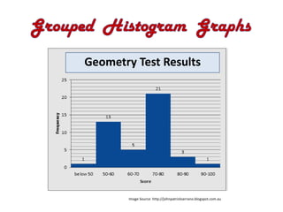
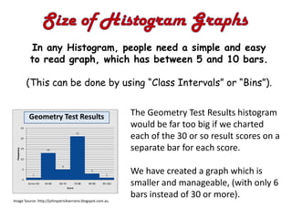
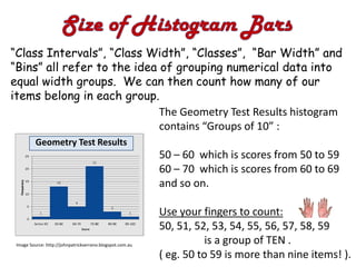
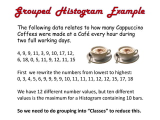
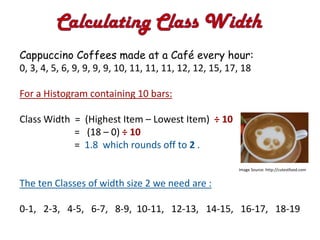
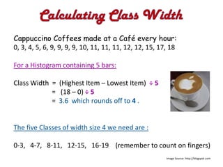
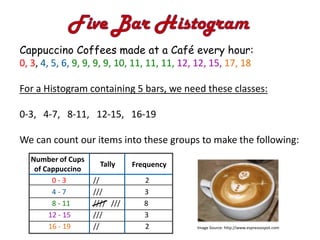
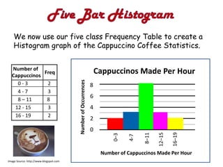
This presentation shows how to draw a Histogram Graph were data is grouped into Class Intervals or Classes.
To obtain a PowerPoint format download of this presentation, go to the following page:
http://passyworldofmathematics.com/pwerpoints/
The document discusses the probability of drawing cards from a standard 52-card deck. It provides three methods to calculate the probability of drawing a flush (5 cards of the same suit) and explains the calculations in each method. The methods yield the same probability of drawing a flush, which is approximately 0.00208 or 1 in 480.
This document provides information about fractions, decimals, and percentages including:
- Examples of how fractions, decimals, and percentages relate and can be converted between each other.
- Steps for converting a fraction to a decimal by dividing the numerator by the denominator.
- How to convert a decimal to a percentage by moving the decimal point two places to the right and adding the percent sign.
- How to convert a percentage to a decimal by moving the decimal point two places to the left and dividing by 100.
- Examples of percentage word problems and how to set them up proportionally to solve.
- Additional tips for working with fractions, decimals, and percentages like when a percentage can be greater than 100%.
The document discusses different ways of representing discrete and continuous data using tables, charts, and graphs. It provides an example of discrete data from "Dave's Car Wash" showing the number and types of cars washed on a Sunday. This data is displayed in a table and frequency chart showing that 20 of the 60 cars washed were white. It then shows this same data represented using a pie chart and bar graph to illustrate different visual representations of the discrete data. The document also provides an example of continuous data recording the volume of water in a filling bath over time, and includes a line graph to represent this continuous data variation.
This document discusses percentages and percent problems. It defines a percentage as a fraction with a denominator of 100. Percentages make it easy to compare quantities. A percent problem has three parts: the amount, the base, and the percent. The amount is part of the whole (base). The percent expresses the ratio of the amount to the base as a percentage. The document provides examples and exercises for identifying these parts and calculating unknown values in percent problems using the formula: Percent = Amount/Base x 100.
A stem and leaf plot is a way to organize and visualize data by splitting each data value into a stem and leaf. The stem represents the most significant digits and the leaves are the least significant digits arranged in ascending order within each stem. This allows one to quickly determine the minimum and maximum values, range, and distribution of the data in a data set through a visual representation. Examples are provided to illustrate stem and leaf plots for test score data and long jump distance data, including how to make comparisons between two data sets using a back-to-back stem and leaf plot.
A pie diagram presents data in the form of a circle partitioned into slices corresponding to different categories. Each category's slice represents its percentage of the total by taking up the appropriate number of degrees out of the full circle's 360 degrees. For example, a pie diagram could show that of 50 students, 5 (10%) were group A, 20 (40%) were group B, 10 (20%) were group AB, and 15 (30%) were group O.
This document discusses the Euclid's algorithm for finding the greatest common divisor (GCD) of two numbers. It begins by explaining the algorithm and providing an example of finding the GCD of 256 and 16. Then it provides 3 additional examples of using the algorithm to find the GCD of various number pairs. The last part asks the reader to find the largest number that divides two given numbers and leaves specific remainders. It walks through applying the Euclid's algorithm to solve this problem.
This document discusses cumulative frequency distribution. It defines cumulative frequency as the frequency of occurrence of values less than a reference value. The document outlines how to build a cumulative frequency distribution table from a frequency table or histogram by summing the frequencies in each class. Cumulative frequency analysis is used to understand how often a phenomenon is below a certain value and can help in describing situations or planning interventions.
This document discusses stem-and-leaf diagrams, line charts, and scatter diagrams. It provides examples and steps for constructing each type of graph. Stem-and-leaf diagrams display and order numerical data using digits in the tens and ones places. Line charts show the relationship between two quantitative variables over time. Scatter diagrams plot the relationship between two quantitative variables to determine if they are correlated. Examples and steps are given for accurately constructing each graph.
Distributive property in algebra power pointChristie Harp
ย
The document discusses the distributive property in algebra. The distributive property allows terms inside parentheses to be distributed so that expressions can be simplified out of order from the standard order of operations. It involves multiplying the number outside of the parentheses by each term inside the parentheses. Examples are provided to demonstrate how to use the distributive property to simplify expressions.
This document provides instruction on calculating measures of variability such as range, quartiles, and creating box-and-whisker plots. It includes examples of finding the range and quartiles for data sets. Additional examples demonstrate how to make box-and-whisker plots from data and compare plots to analyze differences between data sets. Practice problems are provided to have students calculate range, quartiles, and create box-and-whisker plots.
This document defines and provides examples for calculating the mean, median, mode, and range of a data set. It explains that the mean is calculated by adding all values and dividing by the number of values, the median involves ordering values and selecting the middle one, the mode is the most frequent value, and the range is the difference between the highest and lowest values. Examples are given for each statistical measure.
Converting fractions, decimals, and percentsBrittany Bell
ย
This document provides instructions for converting between decimals, percentages, and fractions. It explains that to convert a decimal to a percent, move the decimal point two places to the right and add a percent sign. To convert a percent to a decimal, move the decimal point two places to the left. To convert a fraction to a decimal, divide the numerator by the denominator. And to convert a percent to a fraction, first change it to a decimal and then write the decimal over 100. Examples are given for each type of conversion.
A decimal is a number written in the base ten system, with a decimal point separating the ones place from the tenths place. Places to the right of the decimal point show parts of a whole, with tenths being the first place and hundredths, thousandths, etc following. When ordering decimals from least to greatest, zeros at the end do not change the value, and the number of digits does not matter - only the first digit in each number is compared. Decimals are rounded in the same way as whole numbers, rounding up if above 5 and down if below. Adding and subtracting decimals involves lining up the decimal points and performing the operation as with whole numbers, while multiplying requires multiplying as usual and placing the decimal
This document provides information about different types of graphs, including line graphs and bar graphs. It defines a line graph as a diagram that connects points on an x-y plane to show the relationship between two variables. Bar graphs use vertical or horizontal bars to show comparisons between categories. The document explains the key parts of line graphs and bar graphs, such as the title, labels, scales, points and bars. It also provides steps to construct a line graph using sample data on daily earnings. For bar graphs, it outlines how to create bars of uniform width and height according to a chosen scale. An example bar graph shows the number of children in different activities.
This document discusses different types of graphs used to represent data. It outlines eight main types of graphs: bar graphs, pie charts, tally charts, area graphs, pictographs, waterfall graphs, line graphs, and polar graphs. Each graph type is briefly described, including details about bar graphs having two axes (X and Y), pie charts showing proportional sectors, and waterfall charts representing cumulative positive or negative values. Pictographs use pictures to represent data, while line graphs connect data points with straight lines. The document provides a high-level overview of common graph types used for data visualization.
This document defines and explains different types of numbers:
1. Natural numbers are the positive whole numbers {1, 2, 3...}. Whole numbers include 0. Integers include positive and negative whole numbers. Rational numbers can be written as fractions. Irrational numbers cannot be written as fractions.
2. Real numbers include rational and irrational numbers and can be written as decimals. Complex numbers are numbers in the form a + bi, where a and b are real numbers. Complex numbers contain both real and imaginary parts.
3. The set of complex numbers contains all real and imaginary numbers. Operations on complex numbers follow specific rules: addition/subtraction combine real and imaginary parts separately, multiplication distributes and
The document discusses percentages and methods for calculating percentages of numbers. It provides examples of calculating percentages such as 50%, 10%, 1%, and other percentages by dividing the original number by 2, 10, 100 or using other methods. It also discusses calculating percentages without and with a calculator.
This document provides instructions for performing basic operations with decimals such as addition, subtraction, multiplication, and division. It explains how to align the decimals and describes the steps for each operation. Examples are provided for adding, subtracting, multiplying, and dividing decimals. The document also covers comparing and converting fractions and decimals, with examples of how to convert a fraction to a decimal and vice versa. It concludes with contact information.
This document provides information about percentages including definitions, ways to express parts of a whole as fractions, decimals, percentages or ratios. It gives examples of calculating percentages of quantities, finding percentages of totals, percentage increase and decrease. It discusses percentage change and problems involving population growth/decline rates and depreciation rates. Finally, it presents some example problems involving percentages applied to prices, profits/losses and revenues.
This document contains information about line graphs, including:
1) A line graph uses points connected by lines to show how something changes over time or as another variable changes.
2) Line graphs are used for qualitative data to track changes over short or long periods of time or to compare changes for multiple groups.
3) Examples of qualitative data include hair color, softness of skin, and gender, which can't be directly measured.
This document defines and provides formulas for kurtosis, a statistical measure of the peakedness of a distribution curve. Kurtosis values indicate whether a curve is normal/mesokurtic (Ku=0.263), flat/platykurtic (Ku>0.263), or thin/leptokurtic (Ku<0.263). It also includes an example frequency distribution of examination marks in statistics.
Numbering system, binary number system, octal number system, decimal number system, hexadecimal number system.
Code conversion, Conversion from one number system to another, floating point numbers
Displaying data using charts and graphsCharles Flynt
ย
Bar charts, line graphs, pie charts, scatter plots, and histograms are commonly used types of charts. Each type of chart has distinct characteristics that make it suitable for visualizing certain types of data relationships. Bar charts are useful for comparing discrete categories, line graphs show trends over time, pie charts show proportions, scatter plots reveal correlations between two variables, and histograms display frequency distributions. Proper chart selection and design ensure data is presented clearly and accurately.
This document discusses various measures of dispersion, which refer to how spread out or varied a set of data is from a central value. It describes standard deviation, which quantifies how far data points deviate from the mean on average. A lower standard deviation indicates less volatility or risk. The coefficient of variation allows comparison of volatility relative to expected returns. The range is the maximum minus minimum value but can be skewed by outliers, while the interquartile range ignores the highest and lowest quartiles to better represent the middle data.
Contingency tables, or crosstabs, summarize the relationship between categorical variables. They display counts of observations cross-classified by discrete predictors and response variables. Contingency tables are used to assess if factors are related, describe data frequencies and proportions, and test relationships between factors using chi-square tests. They show counts in each cell, and row, column, and total percentages to understand associations between independent variables like exposures, dependent outcome variables, and potential confounders.
This document provides information about different types of graphs. It defines what a graph is as a two-dimensional drawing that shows the relationship between two sets of numbers using a line, curve, bars, or other symbols. It then describes several common types of graphs: circle graphs that display data in circular sections; bar graphs that use vertical or horizontal bars of equal width; pictographs that use pictures and symbols with a key; broken line graphs that join data points over time with line segments; continuous line graphs where points on the line also have meaning; and scatter plots that show a set of plotted points.
Rational numbers include all integers as well as numbers that can be expressed as fractions p/q where p and q are integers and q is not equal to 0. Rational numbers are closed under addition, subtraction, and multiplication but not division. They have identities and inverses. Rational numbers can be represented on a number line and there are infinite numbers between any two rational numbers that can be found using methods like the mean or equivalent fractions.
1) The document discusses how exponential growth and decay occur in many natural and technological systems.
2) It provides examples of exponential growth such as population growth, fuel consumption, and spread of information through social networks.
3) Exponential decay is also covered through examples like the decrease of radiation over time and reduction of sound and light intensity with distance.
This document provides rules and explanations for operations involving exponents. It discusses:
1) The rule for adding or subtracting exponents with the same base, such as am + n = amxn or am รท an = am-n.
2) Exceptions when the bases are different, such as 23 x m4 โ 2m7.
3) The power of a power rule, such as (n2)4 = n8, which only works for a single positive base in brackets.
4) How to expand products and quotients with the same exponents, such as (2a)2 = 4a2, and simplify fractions with different bases but the same exponents.
The document provides steps for solving equations with fractions that involve the same variable on both sides. It explains that these types of equations cannot be solved using traditional back-tracking methods. The extra steps include: 1) cross multiplying using brackets to remove fractions, 2) identifying the smaller letter term on both sides, and 3) applying the opposite operation to this term on both sides before simplifying and solving as normal. It then works through examples demonstrating these steps, such as solving the equation n-3=n+6/2/3.
This document provides steps for solving equations with variables on both sides:
1. Expand any brackets first.
2. Identify the smaller term with the variable.
3. Apply the opposite operation (+ or -) to that term on both sides.
4. Simplify and solve the resulting equation normally using techniques like onion skins or backtracking.
Worked examples demonstrate subtracting and adding the smaller variable term to move it to one side.
- The gradient or slope represents how steep a slope is, with uphill slopes being positive and downhill slopes being negative.
- The gradient is measured by the rise over the run, where rise is the vertical change in distance and run is the horizontal change in distance between two points.
- To find the gradient between two points, you create a right triangle between the points and calculate the rise as the vertical leg and the run as the horizontal leg, then plug those values into the formula: Gradient = Rise/Run.
The document discusses finding the midpoint between two points on a coordinate grid. It provides examples of using the midpoint formula, which is (x1 + x2)/2 for the x-coordinate and (y1 + y2)/2 for the y-coordinate, where (x1, y1) are the coordinates of the first point and (x2, y2) are the coordinates of the second point. It also presents an alternative method of adding the x- and y-coordinates of the two points separately and dividing each sum by two.
This document discusses linear relationships and rules for determining the relationship between x and y values in a table. There are three main types of linear rules: 1) simple addition or subtraction, 2) simple multiplication or division, and 3) combination rules using y=mx+c. To determine the rule, you first check if it follows addition/subtraction by looking for a consistent difference between y-x values. If not, you check for multiplication/division by looking at y/x values. If neither, it uses a combination rule where you calculate the slope m from the change in y over change in x, use a point to find the y-intercept c, then write the rule as y=mx+c. Examples
The document describes how to create a back-to-back stem and leaf plot to compare the battery life data from two phone brands. It shows the raw battery life data for each brand in hours. Then it draws individual stem and leaf plots for each brand's data. Finally, it combines the two plots by reversing one and placing them side by side to allow direct comparison of the battery life distributions between the two brands.
The document discusses different types of distributions in graphs of test score data:
- Positive skew occurs when a small number of high scores stretch the graph out to the right, with the mean higher than the median and mode.
- Negative skew is the opposite, with a small number of low scores stretching the graph left and the mean lower than the median and mode.
- A symmetrical distribution has scores evenly distributed on both sides of the median, with the mean, median and mode close together.
A coffee shop conducted a two-day survey to determine the average number of cappuccinos made per hour. A histogram showed the frequency of cappuccinos made within various hourly intervals. To calculate the average, interval midpoints were determined and multiplied by the frequencies. The total of these products was divided by the total frequency, determining that the average number of cappuccinos made per hour was 10.
After take-off, planes ascend at an angle to reach their cruising altitude. This angle of elevation is related to the opposite and adjacent sides of a right triangle through the tangent ratio, which is the opposite side divided by the adjacent side. For any right triangle with the same angle, the tangent ratio of opposite over adjacent will be the same value. Solving tangent triangle problems involves labeling sides, determining what is unknown (opposite, adjacent, or angle), and using the appropriate tangent formula along with a calculator set to degrees mode.
The document discusses the relationship between trigonometric functions like sine and cosine waves and sound waves. It explains that distorted heavy metal guitar sounds occur when smooth sine and cosine waves are transformed into square, sawtooth, or triangle waves. It then provides instructions and examples for using cosine functions to solve right triangle problems, including determining unknown side lengths or angles using special calculator buttons.
When a plane descends for landing, its flight path forms a right triangle with its speed and angle determining the hypotenuse. There are four formulas for working with sine triangles: opposite side equals hypotenuse multiplied by sine of the angle; angle equals inverse sine of opposite over hypotenuse; hypotenuse equals opposite divided by sine of the angle; and calculators use the sine and inverse sine buttons set to degrees mode. Solving sine triangle problems involves labeling sides, identifying the unknown, and applying the appropriate formula while substituting values and rounding answers.
This document discusses the mathematics behind similar triangles and their use in calculating unknown heights or lengths. It provides examples of using scale factors to determine the height of tall objects from shadow lengths. Similar triangles are used when two triangles share the same angle measures or their angles are vertical angles. The scale factor is set up as a ratio of corresponding sides between the two triangles. Cross multiplying the scale factor equation allows the calculation of unknown sides or heights.
The document discusses similar triangles and scale factors. It provides examples of similar triangles in nature, art, architecture, and mathematics. It explains the different rules to determine if triangles are similar: AAA (angle-angle-angle), PPP (proportional property), PAP (proportional angles property), and RHS (right-hypotenuse-side). Examples are given applying these rules to prove triangles are similar and calculate missing side lengths or scale factors.
This document provides an overview of congruent triangles and the different rules that can be used to prove triangles are congruent. It defines congruent triangles as triangles that have the same size and shape. It then presents four main rules for proving triangles are congruent: 1) three sides are equal (SSS rule), 2) two sides and the included angle are equal (SAS rule), 3) two angles and a non-included side are equal (AAS rule), and 4) a right angle, hypotenuse, and one other side are equal (RHS rule). The document explains each rule and provides examples of how to apply them to identify matching elements and prove triangles congruent.
This document discusses finding the common factor of algebraic expressions. It explains that to find the common factor, one must break down all numbers within the expressions into their prime number factors. The common factors that are present in both expressions are then written outside of parentheses, while the remaining terms are written inside. Several examples are provided of factorizing expressions using this process of identifying common prime factors. The "highest common factor" refers to the largest common factor present outside of the parentheses.
Expanding binomial expressions is an important mathematical skill used in graphing parabolic shapes like the Sydney Harbour Bridge. There are two methods for expanding binomial expressions: using the order of operations (BODMAS/PEMDAS) or using the binomial expansion/FOIL method. Examples show how to apply the distribution property to expand binomial expressions with two, three, or four terms in the result. Expanding binomials is a fundamental skill needed for more advanced mathematics.
The document discusses the "onion skin" method for transposing (rearranging) algebra formula equations. It explains that with this method, you draw concentric "skins" or circles around the equation, starting with the variable you want to isolate. You then work inward by applying the opposite operations to each term or part of the equation until the desired variable is alone on one side. It provides examples of using this method to transpose different types of equations, including ones with fractions, exponents, multiple variables, and square roots.
Leveraging Generative AI to Drive Nonprofit InnovationTechSoup
ย
In this webinar, participants learned how to utilize Generative AI to streamline operations and elevate member engagement. Amazon Web Service experts provided a customer specific use cases and dived into low/no-code tools that are quick and easy to deploy through Amazon Web Service (AWS.)
Temple of Asclepius in Thrace. Excavation resultsKrassimira Luka
ย
The temple and the sanctuary around were dedicated to Asklepios Zmidrenus. This name has been known since 1875 when an inscription dedicated to him was discovered in Rome. The inscription is dated in 227 AD and was left by soldiers originating from the city of Philippopolis (modern Plovdiv).
Walmart Business+ and Spark Good for Nonprofits.pdfTechSoup
ย
"Learn about all the ways Walmart supports nonprofit organizations.
You will hear from Liz Willett, the Head of Nonprofits, and hear about what Walmart is doing to help nonprofits, including Walmart Business and Spark Good. Walmart Business+ is a new offer for nonprofits that offers discounts and also streamlines nonprofits order and expense tracking, saving time and money.
The webinar may also give some examples on how nonprofits can best leverage Walmart Business+.
The event will cover the following::
Walmart Business + (https://business.walmart.com/plus) is a new shopping experience for nonprofits, schools, and local business customers that connects an exclusive online shopping experience to stores. Benefits include free delivery and shipping, a 'Spend Analyticsโ feature, special discounts, deals and tax-exempt shopping.
Special TechSoup offer for a free 180 days membership, and up to $150 in discounts on eligible orders.
Spark Good (walmart.com/sparkgood) is a charitable platform that enables nonprofits to receive donations directly from customers and associates.
Answers about how you can do more with Walmart!"
A Visual Guide to 1 Samuel | A Tale of Two HeartsSteve Thomason
ย
These slides walk through the story of 1 Samuel. Samuel is the last judge of Israel. The people reject God and want a king. Saul is anointed as the first king, but he is not a good king. David, the shepherd boy is anointed and Saul is envious of him. David shows honor while Saul continues to self destruct.
Philippine Edukasyong Pantahanan at Pangkabuhayan (EPP) CurriculumMJDuyan
ย
(๐๐๐ ๐๐๐) (๐๐๐ฌ๐ฌ๐จ๐ง ๐)-๐๐ซ๐๐ฅ๐ข๐ฆ๐ฌ
๐๐ข๐ฌ๐๐ฎ๐ฌ๐ฌ ๐ญ๐ก๐ ๐๐๐ ๐๐ฎ๐ซ๐ซ๐ข๐๐ฎ๐ฅ๐ฎ๐ฆ ๐ข๐ง ๐ญ๐ก๐ ๐๐ก๐ข๐ฅ๐ข๐ฉ๐ฉ๐ข๐ง๐๐ฌ:
- Understand the goals and objectives of the Edukasyong Pantahanan at Pangkabuhayan (EPP) curriculum, recognizing its importance in fostering practical life skills and values among students. Students will also be able to identify the key components and subjects covered, such as agriculture, home economics, industrial arts, and information and communication technology.
๐๐ฑ๐ฉ๐ฅ๐๐ข๐ง ๐ญ๐ก๐ ๐๐๐ญ๐ฎ๐ซ๐ ๐๐ง๐ ๐๐๐จ๐ฉ๐ ๐จ๐ ๐๐ง ๐๐ง๐ญ๐ซ๐๐ฉ๐ซ๐๐ง๐๐ฎ๐ซ:
-Define entrepreneurship, distinguishing it from general business activities by emphasizing its focus on innovation, risk-taking, and value creation. Students will describe the characteristics and traits of successful entrepreneurs, including their roles and responsibilities, and discuss the broader economic and social impacts of entrepreneurial activities on both local and global scales.
This presentation was provided by Rebecca Benner, Ph.D., of the American Society of Anesthesiologists, for the second session of NISO's 2024 Training Series "DEIA in the Scholarly Landscape." Session Two: 'Expanding Pathways to Publishing Careers,' was held June 13, 2024.
ISO/IEC 27001, ISO/IEC 42001, and GDPR: Best Practices for Implementation and...PECB
ย
Denis is a dynamic and results-driven Chief Information Officer (CIO) with a distinguished career spanning information systems analysis and technical project management. With a proven track record of spearheading the design and delivery of cutting-edge Information Management solutions, he has consistently elevated business operations, streamlined reporting functions, and maximized process efficiency.
Certified as an ISO/IEC 27001: Information Security Management Systems (ISMS) Lead Implementer, Data Protection Officer, and Cyber Risks Analyst, Denis brings a heightened focus on data security, privacy, and cyber resilience to every endeavor.
His expertise extends across a diverse spectrum of reporting, database, and web development applications, underpinned by an exceptional grasp of data storage and virtualization technologies. His proficiency in application testing, database administration, and data cleansing ensures seamless execution of complex projects.
What sets Denis apart is his comprehensive understanding of Business and Systems Analysis technologies, honed through involvement in all phases of the Software Development Lifecycle (SDLC). From meticulous requirements gathering to precise analysis, innovative design, rigorous development, thorough testing, and successful implementation, he has consistently delivered exceptional results.
Throughout his career, he has taken on multifaceted roles, from leading technical project management teams to owning solutions that drive operational excellence. His conscientious and proactive approach is unwavering, whether he is working independently or collaboratively within a team. His ability to connect with colleagues on a personal level underscores his commitment to fostering a harmonious and productive workplace environment.
Date: May 29, 2024
Tags: Information Security, ISO/IEC 27001, ISO/IEC 42001, Artificial Intelligence, GDPR
-------------------------------------------------------------------------------
Find out more about ISO training and certification services
Training: ISO/IEC 27001 Information Security Management System - EN | PECB
ISO/IEC 42001 Artificial Intelligence Management System - EN | PECB
General Data Protection Regulation (GDPR) - Training Courses - EN | PECB
Webinars: https://pecb.com/webinars
Article: https://pecb.com/article
-------------------------------------------------------------------------------
For more information about PECB:
Website: https://pecb.com/
LinkedIn: https://www.linkedin.com/company/pecb/
Facebook: https://www.facebook.com/PECBInternational/
Slideshare: http://www.slideshare.net/PECBCERTIFICATION
2. In any Histogram, people need a simple and easy
to read graph, which has between 5 and 10 bars.
(This can be done by using โClass Intervalsโ or โBinsโ).
Geometry Test Results The Geometry Test Results histogram
would be far too big if we charted
each of the 30 or so result scores on a
separate bar for each score.
We have created a graph which is
smaller and manageable, (with only 6
bars instead of 30 or more).
Image Source: http://johnpatrickserrano.blogspot.com.au
3. โClass Intervalsโ, โClass Widthโ, โClassesโ, โBar Widthโ and
โBinsโ all refer to the idea of grouping numerical data into
equal width groups. We can then count how many of our
items belong in each group.
The Geometry Test Results histogram
contains โGroups of 10โ :
Geometry Test Results
50 โ 60 which is scores from 50 to 59
60 โ 70 which is scores from 60 to 69
and so on.
Use your fingers to count:
50, 51, 52, 53, 54, 55, 56, 57, 58, 59
Image Source: http://johnpatrickserrano.blogspot.com.au
is a group of TEN .
( eg. 50 to 59 is more than nine items! ).
4. The following data relates to how many Cappuccino
Coffees were made at a Cafรฉ every hour during
two full working days.
4, 9, 9, 11, 3, 9, 10, 17, 12,
6, 18, 0, 5, 11, 9, 12, 11, 15
First we rewrite the numbers from lowest to highest:
0, 3, 4, 5, 6, 9, 9, 9, 9, 10, 11, 11, 11, 12, 12, 15, 17, 18
We have 12 different number values, but ten different
values is the maximum for a Histogram containing 10 bars.
So we need to do grouping into โClassesโ to reduce this.
5. Cappuccino Coffees made at a Cafรฉ every hour:
0, 3, 4, 5, 6, 9, 9, 9, 9, 10, 11, 11, 11, 12, 12, 15, 17, 18
For a Histogram containing 10 bars:
Class Width = (Highest Item โ Lowest Item) รท 10
= (18 โ 0) รท 10
= 1.8 which rounds off to 2 .
Image Source: http://cutestfood.com
The ten Classes of width size 2 we need are :
0-1, 2-3, 4-5, 6-7, 8-9, 10-11, 12-13, 14-15, 16-17, 18-19
6. Cappuccino Coffees made at a Cafรฉ every hour:
0, 3, 4, 5, 6, 9, 9, 9, 9, 10, 11, 11, 11, 12, 12, 15, 17, 18
For a Histogram containing 5 bars:
Class Width = (Highest Item โ Lowest Item) รท 5
= (18 โ 0) รท 5
= 3.6 which rounds off to 4 .
The five Classes of width size 4 we need are :
0-3, 4-7, 8-11, 12-15, 16-19 (remember to count on fingers)
Image Source: http://blogspot.com
7. Cappuccino Coffees made at a Cafรฉ every hour:
0, 3, 4, 5, 6, 9, 9, 9, 9, 10, 11, 11, 11, 12, 12, 15, 17, 18
For a Histogram containing 5 bars, we need these classes:
0-3, 4-7, 8-11, 12-15, 16-19
We can count our items into these groups to make the following:
Number of Cups
Tally Frequency
of Cappuccino
0-3 // 2
4-7 /// 3
8 - 11 //// /// 8
12 - 15 /// 3
16 - 19 // 2 Image Source: http://www.espressospot.com
8. We now use our five class Frequency Table to create a
Histogram graph of the Cappuccino Coffee Statistics.
Number of
Freq
Cappuccinos
0-3 2 8
4-7 3
6
8 โ 11 8
12 - 15 3 4
16 - 19 2
2
0
0โ3
Number of Cappuccinos Made Per Hour
Image Source: http://www.blogspot.com