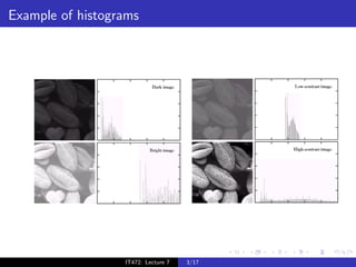
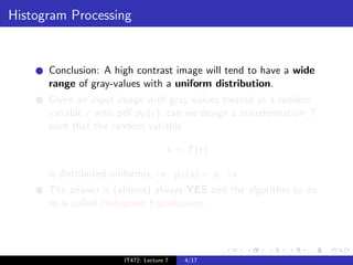
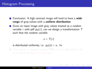
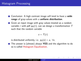
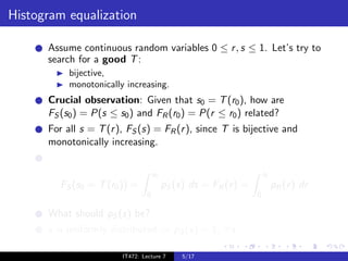
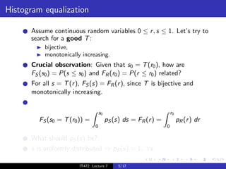
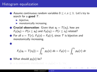
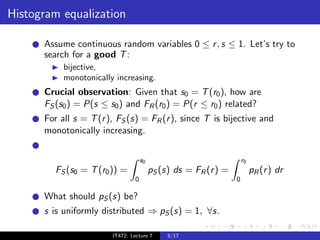
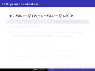
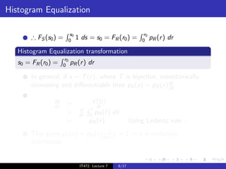
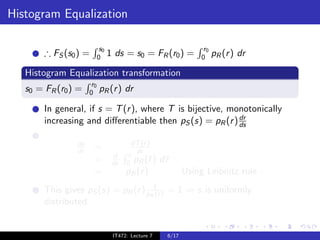
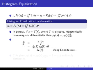
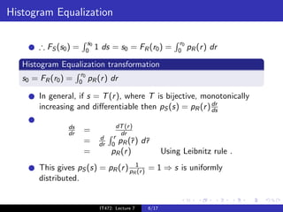
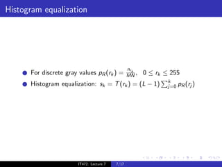
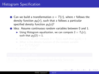
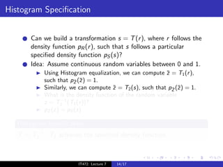
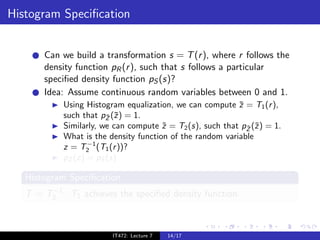
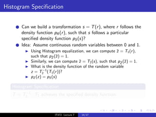
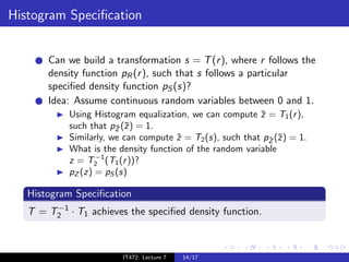
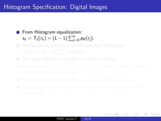
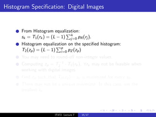
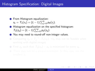
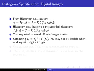
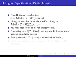
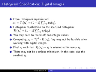
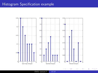
Histogram Processing

IT 472: Digital Image Processing, Lecture 7
Histogram


      The i th histogram entry for a digital image is
                                M     N
                          1
              h(ri ) =                        χri (f [i, j]),   0 ≤ ri ≤ L − 1,
                         MN
                               i=1 j=1

      where

                         χri (f [i, j]) = 1               if f [i, j] = ri
                                              = 0 otherwise

      Estimates the probability distribution function of gray values
      in an image.
      Gives a good idea of contrast in an image.


                           IT472: Lecture 7        2/17
Example of histograms


                  IT472: Lecture 7   3/17
Histogram Processing


      Conclusion: A high contrast image will tend to have a wide
      range of gray-values with a uniform distribution.
      Given an input image with gray values treated as a random
      variable r with pdf pR (r ), can we design a transformation T
      such that the random variable

                                       s = T (r )

      is distributed uniformly, i.e. pS (s) = a, ∀s.
      The answer is (almost) always YES and the algorithm to do
      so is called Histogram Equalization.


                        IT472: Lecture 7   4/17
Histogram equalization

      Assume continuous random variables 0 ≤ r , s ≤ 1. Let’s try to
      search for a good T :
           bijective,
           monotonically increasing.
      Crucial observation: Given that s0 = T (r0 ), how are
      FS (s0 ) = P(s ≤ s0 ) and FR (r0 ) = P(r ≤ r0 ) related?
      For all s = T (r ), FS (s) = FR (r ), since T is bijective and
      monotonically increasing.


                                     s0                               r0
         FS (s0 = T (r0 )) =              pS (s) ds = FR (r ) =            pR (r ) dr
                                 0                                0

      What should pS (s) be?
      s is uniformly distributed ⇒ pS (s) = 1, ∀s.

                        IT472: Lecture 7       5/17
Histogram Equalization

                            s0                                     r0
        ∴ FS (s0 ) =       0     1 ds = s0 = FR (r0 ) =           0     pR (r ) dr

   Histogram Equalization transformation
                      r0
   s0 = FR (r0 ) =   0     pR (r ) dr

        In general, if s = T (r ), where T is bijective, monotonically
                                                           dr
        increasing and differentiable then pS (s) = pR (r ) ds

                ds                       dT (r )
                dr     =                  dr
                                  d     r
                       =          dr   0 pR (¯)r     d¯
                                                      r
                       =               pR (r )               Using Leibnitz rule .
        This gives pS (s) = pR (r ) pR1 ) = 1 ⇒ s is uniformly
                                      (r
        distributed.


                                  IT472: Lecture 7    6/17
Histogram equalization


                                                 nrk
      For discrete gray values pR (rk ) =        MN ,   0 ≤ rk ≤ 255
                                                                k
      Histogram equalization: sk = T (rk ) = (L − 1)            j=0 pR (rj )


                       IT472: Lecture 7   7/17
Examples


           IT472: Lecture 7   8/17
Examples


           IT472: Lecture 7   9/17
Histogram Equalization


      What happens if we apply histogram equalization twice on an
      image?
      Histogram equalization is idempotent!


                      IT472: Lecture 7   10/17
Histogram Equalization


      What happens if we apply histogram equalization twice on an
      image?
      Histogram equalization is idempotent!


                      IT472: Lecture 7   10/17
Histogram Equalization issues


                   IT472: Lecture 7   11/17
Histogram Equalization issues


                   IT472: Lecture 7   12/17
Histogram Specification


                  IT472: Lecture 7   13/17
Histogram Specification


       Can we build a transformation s = T (r ), where r follows the
       density function pR (r ), such that s follows a particular
       specified density function pS (s)?
       Idea: Assume continuous random variables between 0 and 1.
            Using Histogram equalization, we can compute z = T1 (r ),
                                                           ¯
            such that pZ (¯) = 1.
                        ¯ z
            Similarly, we can compute z = T2 (s), such that pZ (˜) = 1.
                                       ˜                     ˜ z
            What is the density function of the random variable
                   −1
            z = T2 (T1 (r ))?
            pZ (z) = pS (s)

   Histogram Specification
        −1
   T = T2 · T1 achieves the specified density function.


                         IT472: Lecture 7   14/17
Histogram Specification: Digital Images


      From Histogram equalization:
      sk = T1 (rk ) = (L − 1) k pR (rj ).
                              j=0
      Histogram equalization on the specified histogram:
      T2 (zp ) = (L − 1) p pZ (zp )
                         i=0
      You may need to round-off non-integer values.
                         −1
      Computing zp = T2 · T1 (rk ), ∀rk may not be feasible when
      working with digital images.
      Find zp such that T2 (zp ) − sk is minimized for every sk .
      There may not be a unique minimizer. In this case, use the
      smallest sk .


                       IT472: Lecture 7   15/17
Histogram Specification example


                  IT472: Lecture 7   16/17
Histogram Specification example


                  IT472: Lecture 7   17/17

Image Processing 4

  • 1.
    Histogram Processing IT 472:Digital Image Processing, Lecture 7
  • 2.
    Histogram The i th histogram entry for a digital image is M N 1 h(ri ) = χri (f [i, j]), 0 ≤ ri ≤ L − 1, MN i=1 j=1 where χri (f [i, j]) = 1 if f [i, j] = ri = 0 otherwise Estimates the probability distribution function of gray values in an image. Gives a good idea of contrast in an image. IT472: Lecture 7 2/17
  • 3.
    Histogram The i th histogram entry for a digital image is M N 1 h(ri ) = χri (f [i, j]), 0 ≤ ri ≤ L − 1, MN i=1 j=1 where χri (f [i, j]) = 1 if f [i, j] = ri = 0 otherwise Estimates the probability distribution function of gray values in an image. Gives a good idea of contrast in an image. IT472: Lecture 7 2/17
  • 4.
    Histogram The i th histogram entry for a digital image is M N 1 h(ri ) = χri (f [i, j]), 0 ≤ ri ≤ L − 1, MN i=1 j=1 where χri (f [i, j]) = 1 if f [i, j] = ri = 0 otherwise Estimates the probability distribution function of gray values in an image. Gives a good idea of contrast in an image. IT472: Lecture 7 2/17
  • 5.
    Example of histograms IT472: Lecture 7 3/17
  • 6.
    Histogram Processing Conclusion: A high contrast image will tend to have a wide range of gray-values with a uniform distribution. Given an input image with gray values treated as a random variable r with pdf pR (r ), can we design a transformation T such that the random variable s = T (r ) is distributed uniformly, i.e. pS (s) = a, ∀s. The answer is (almost) always YES and the algorithm to do so is called Histogram Equalization. IT472: Lecture 7 4/17
  • 7.
    Histogram Processing Conclusion: A high contrast image will tend to have a wide range of gray-values with a uniform distribution. Given an input image with gray values treated as a random variable r with pdf pR (r ), can we design a transformation T such that the random variable s = T (r ) is distributed uniformly, i.e. pS (s) = a, ∀s. The answer is (almost) always YES and the algorithm to do so is called Histogram Equalization. IT472: Lecture 7 4/17
  • 8.
    Histogram Processing Conclusion: A high contrast image will tend to have a wide range of gray-values with a uniform distribution. Given an input image with gray values treated as a random variable r with pdf pR (r ), can we design a transformation T such that the random variable s = T (r ) is distributed uniformly, i.e. pS (s) = a, ∀s. The answer is (almost) always YES and the algorithm to do so is called Histogram Equalization. IT472: Lecture 7 4/17
  • 9.
    Histogram equalization Assume continuous random variables 0 ≤ r , s ≤ 1. Let’s try to search for a good T : bijective, monotonically increasing. Crucial observation: Given that s0 = T (r0 ), how are FS (s0 ) = P(s ≤ s0 ) and FR (r0 ) = P(r ≤ r0 ) related? For all s = T (r ), FS (s) = FR (r ), since T is bijective and monotonically increasing. s0 r0 FS (s0 = T (r0 )) = pS (s) ds = FR (r ) = pR (r ) dr 0 0 What should pS (s) be? s is uniformly distributed ⇒ pS (s) = 1, ∀s. IT472: Lecture 7 5/17
  • 10.
    Histogram equalization Assume continuous random variables 0 ≤ r , s ≤ 1. Let’s try to search for a good T : bijective, monotonically increasing. Crucial observation: Given that s0 = T (r0 ), how are FS (s0 ) = P(s ≤ s0 ) and FR (r0 ) = P(r ≤ r0 ) related? For all s = T (r ), FS (s) = FR (r ), since T is bijective and monotonically increasing. s0 r0 FS (s0 = T (r0 )) = pS (s) ds = FR (r ) = pR (r ) dr 0 0 What should pS (s) be? s is uniformly distributed ⇒ pS (s) = 1, ∀s. IT472: Lecture 7 5/17
  • 11.
    Histogram equalization Assume continuous random variables 0 ≤ r , s ≤ 1. Let’s try to search for a good T : bijective, monotonically increasing. Crucial observation: Given that s0 = T (r0 ), how are FS (s0 ) = P(s ≤ s0 ) and FR (r0 ) = P(r ≤ r0 ) related? For all s = T (r ), FS (s) = FR (r ), since T is bijective and monotonically increasing. s0 r0 FS (s0 = T (r0 )) = pS (s) ds = FR (r ) = pR (r ) dr 0 0 What should pS (s) be? s is uniformly distributed ⇒ pS (s) = 1, ∀s. IT472: Lecture 7 5/17
  • 12.
    Histogram equalization Assume continuous random variables 0 ≤ r , s ≤ 1. Let’s try to search for a good T : bijective, monotonically increasing. Crucial observation: Given that s0 = T (r0 ), how are FS (s0 ) = P(s ≤ s0 ) and FR (r0 ) = P(r ≤ r0 ) related? For all s = T (r ), FS (s) = FR (r ), since T is bijective and monotonically increasing. s0 r0 FS (s0 = T (r0 )) = pS (s) ds = FR (r ) = pR (r ) dr 0 0 What should pS (s) be? s is uniformly distributed ⇒ pS (s) = 1, ∀s. IT472: Lecture 7 5/17
  • 13.
    Histogram equalization Assume continuous random variables 0 ≤ r , s ≤ 1. Let’s try to search for a good T : bijective, monotonically increasing. Crucial observation: Given that s0 = T (r0 ), how are FS (s0 ) = P(s ≤ s0 ) and FR (r0 ) = P(r ≤ r0 ) related? For all s = T (r ), FS (s) = FR (r ), since T is bijective and monotonically increasing. s0 r0 FS (s0 = T (r0 )) = pS (s) ds = FR (r ) = pR (r ) dr 0 0 What should pS (s) be? s is uniformly distributed ⇒ pS (s) = 1, ∀s. IT472: Lecture 7 5/17
  • 14.
    Histogram equalization Assume continuous random variables 0 ≤ r , s ≤ 1. Let’s try to search for a good T : bijective, monotonically increasing. Crucial observation: Given that s0 = T (r0 ), how are FS (s0 ) = P(s ≤ s0 ) and FR (r0 ) = P(r ≤ r0 ) related? For all s = T (r ), FS (s) = FR (r ), since T is bijective and monotonically increasing. s0 r0 FS (s0 = T (r0 )) = pS (s) ds = FR (r ) = pR (r ) dr 0 0 What should pS (s) be? s is uniformly distributed ⇒ pS (s) = 1, ∀s. IT472: Lecture 7 5/17
  • 15.
    Histogram equalization Assume continuous random variables 0 ≤ r , s ≤ 1. Let’s try to search for a good T : bijective, monotonically increasing. Crucial observation: Given that s0 = T (r0 ), how are FS (s0 ) = P(s ≤ s0 ) and FR (r0 ) = P(r ≤ r0 ) related? For all s = T (r ), FS (s) = FR (r ), since T is bijective and monotonically increasing. s0 r0 FS (s0 = T (r0 )) = pS (s) ds = FR (r ) = pR (r ) dr 0 0 What should pS (s) be? s is uniformly distributed ⇒ pS (s) = 1, ∀s. IT472: Lecture 7 5/17
  • 16.
    Histogram equalization Assume continuous random variables 0 ≤ r , s ≤ 1. Let’s try to search for a good T : bijective, monotonically increasing. Crucial observation: Given that s0 = T (r0 ), how are FS (s0 ) = P(s ≤ s0 ) and FR (r0 ) = P(r ≤ r0 ) related? For all s = T (r ), FS (s) = FR (r ), since T is bijective and monotonically increasing. s0 r0 FS (s0 = T (r0 )) = pS (s) ds = FR (r ) = pR (r ) dr 0 0 What should pS (s) be? s is uniformly distributed ⇒ pS (s) = 1, ∀s. IT472: Lecture 7 5/17
  • 17.
    Histogram Equalization s0 r0 ∴ FS (s0 ) = 0 1 ds = s0 = FR (r0 ) = 0 pR (r ) dr Histogram Equalization transformation r0 s0 = FR (r0 ) = 0 pR (r ) dr In general, if s = T (r ), where T is bijective, monotonically dr increasing and differentiable then pS (s) = pR (r ) ds ds dT (r ) dr = dr d r = dr 0 pR (¯)r d¯ r = pR (r ) Using Leibnitz rule . This gives pS (s) = pR (r ) pR1 ) = 1 ⇒ s is uniformly (r distributed. IT472: Lecture 7 6/17
  • 18.
    Histogram Equalization s0 r0 ∴ FS (s0 ) = 0 1 ds = s0 = FR (r0 ) = 0 pR (r ) dr Histogram Equalization transformation r0 s0 = FR (r0 ) = 0 pR (r ) dr In general, if s = T (r ), where T is bijective, monotonically dr increasing and differentiable then pS (s) = pR (r ) ds ds dT (r ) dr = dr d r = dr 0 pR (¯)r d¯ r = pR (r ) Using Leibnitz rule . This gives pS (s) = pR (r ) pR1 ) = 1 ⇒ s is uniformly (r distributed. IT472: Lecture 7 6/17
  • 19.
    Histogram Equalization s0 r0 ∴ FS (s0 ) = 0 1 ds = s0 = FR (r0 ) = 0 pR (r ) dr Histogram Equalization transformation r0 s0 = FR (r0 ) = 0 pR (r ) dr In general, if s = T (r ), where T is bijective, monotonically dr increasing and differentiable then pS (s) = pR (r ) ds ds dT (r ) dr = dr d r = dr 0 pR (¯)r d¯ r = pR (r ) Using Leibnitz rule . This gives pS (s) = pR (r ) pR1 ) = 1 ⇒ s is uniformly (r distributed. IT472: Lecture 7 6/17
  • 20.
    Histogram Equalization s0 r0 ∴ FS (s0 ) = 0 1 ds = s0 = FR (r0 ) = 0 pR (r ) dr Histogram Equalization transformation r0 s0 = FR (r0 ) = 0 pR (r ) dr In general, if s = T (r ), where T is bijective, monotonically dr increasing and differentiable then pS (s) = pR (r ) ds ds dT (r ) dr = dr d r = dr 0 pR (¯)r d¯ r = pR (r ) Using Leibnitz rule . This gives pS (s) = pR (r ) pR1 ) = 1 ⇒ s is uniformly (r distributed. IT472: Lecture 7 6/17
  • 21.
    Histogram Equalization s0 r0 ∴ FS (s0 ) = 0 1 ds = s0 = FR (r0 ) = 0 pR (r ) dr Histogram Equalization transformation r0 s0 = FR (r0 ) = 0 pR (r ) dr In general, if s = T (r ), where T is bijective, monotonically dr increasing and differentiable then pS (s) = pR (r ) ds ds dT (r ) dr = dr d r = dr 0 pR (¯)r d¯ r = pR (r ) Using Leibnitz rule . This gives pS (s) = pR (r ) pR1 ) = 1 ⇒ s is uniformly (r distributed. IT472: Lecture 7 6/17
  • 22.
    Histogram equalization nrk For discrete gray values pR (rk ) = MN , 0 ≤ rk ≤ 255 k Histogram equalization: sk = T (rk ) = (L − 1) j=0 pR (rj ) IT472: Lecture 7 7/17
  • 23.
    Histogram equalization nrk For discrete gray values pR (rk ) = MN , 0 ≤ rk ≤ 255 k Histogram equalization: sk = T (rk ) = (L − 1) j=0 pR (rj ) IT472: Lecture 7 7/17
  • 24.
    Examples IT472: Lecture 7 8/17
  • 25.
    Examples IT472: Lecture 7 9/17
  • 26.
    Histogram Equalization What happens if we apply histogram equalization twice on an image? Histogram equalization is idempotent! IT472: Lecture 7 10/17
  • 27.
    Histogram Equalization What happens if we apply histogram equalization twice on an image? Histogram equalization is idempotent! IT472: Lecture 7 10/17
  • 28.
    Histogram Equalization issues IT472: Lecture 7 11/17
  • 29.
    Histogram Equalization issues IT472: Lecture 7 12/17
  • 30.
    Histogram Specification IT472: Lecture 7 13/17
  • 31.
    Histogram Specification Can we build a transformation s = T (r ), where r follows the density function pR (r ), such that s follows a particular specified density function pS (s)? Idea: Assume continuous random variables between 0 and 1. Using Histogram equalization, we can compute z = T1 (r ), ¯ such that pZ (¯) = 1. ¯ z Similarly, we can compute z = T2 (s), such that pZ (˜) = 1. ˜ ˜ z What is the density function of the random variable −1 z = T2 (T1 (r ))? pZ (z) = pS (s) Histogram Specification −1 T = T2 · T1 achieves the specified density function. IT472: Lecture 7 14/17
  • 32.
    Histogram Specification Can we build a transformation s = T (r ), where r follows the density function pR (r ), such that s follows a particular specified density function pS (s)? Idea: Assume continuous random variables between 0 and 1. Using Histogram equalization, we can compute z = T1 (r ), ¯ such that pZ (¯) = 1. ¯ z Similarly, we can compute z = T2 (s), such that pZ (˜) = 1. ˜ ˜ z What is the density function of the random variable −1 z = T2 (T1 (r ))? pZ (z) = pS (s) Histogram Specification −1 T = T2 · T1 achieves the specified density function. IT472: Lecture 7 14/17
  • 33.
    Histogram Specification Can we build a transformation s = T (r ), where r follows the density function pR (r ), such that s follows a particular specified density function pS (s)? Idea: Assume continuous random variables between 0 and 1. Using Histogram equalization, we can compute z = T1 (r ), ¯ such that pZ (¯) = 1. ¯ z Similarly, we can compute z = T2 (s), such that pZ (˜) = 1. ˜ ˜ z What is the density function of the random variable −1 z = T2 (T1 (r ))? pZ (z) = pS (s) Histogram Specification −1 T = T2 · T1 achieves the specified density function. IT472: Lecture 7 14/17
  • 34.
    Histogram Specification Can we build a transformation s = T (r ), where r follows the density function pR (r ), such that s follows a particular specified density function pS (s)? Idea: Assume continuous random variables between 0 and 1. Using Histogram equalization, we can compute z = T1 (r ), ¯ such that pZ (¯) = 1. ¯ z Similarly, we can compute z = T2 (s), such that pZ (˜) = 1. ˜ ˜ z What is the density function of the random variable −1 z = T2 (T1 (r ))? pZ (z) = pS (s) Histogram Specification −1 T = T2 · T1 achieves the specified density function. IT472: Lecture 7 14/17
  • 35.
    Histogram Specification Can we build a transformation s = T (r ), where r follows the density function pR (r ), such that s follows a particular specified density function pS (s)? Idea: Assume continuous random variables between 0 and 1. Using Histogram equalization, we can compute z = T1 (r ), ¯ such that pZ (¯) = 1. ¯ z Similarly, we can compute z = T2 (s), such that pZ (˜) = 1. ˜ ˜ z What is the density function of the random variable −1 z = T2 (T1 (r ))? pZ (z) = pS (s) Histogram Specification −1 T = T2 · T1 achieves the specified density function. IT472: Lecture 7 14/17
  • 36.
    Histogram Specification Can we build a transformation s = T (r ), where r follows the density function pR (r ), such that s follows a particular specified density function pS (s)? Idea: Assume continuous random variables between 0 and 1. Using Histogram equalization, we can compute z = T1 (r ), ¯ such that pZ (¯) = 1. ¯ z Similarly, we can compute z = T2 (s), such that pZ (˜) = 1. ˜ ˜ z What is the density function of the random variable −1 z = T2 (T1 (r ))? pZ (z) = pS (s) Histogram Specification −1 T = T2 · T1 achieves the specified density function. IT472: Lecture 7 14/17
  • 37.
    Histogram Specification Can we build a transformation s = T (r ), where r follows the density function pR (r ), such that s follows a particular specified density function pS (s)? Idea: Assume continuous random variables between 0 and 1. Using Histogram equalization, we can compute z = T1 (r ), ¯ such that pZ (¯) = 1. ¯ z Similarly, we can compute z = T2 (s), such that pZ (˜) = 1. ˜ ˜ z What is the density function of the random variable −1 z = T2 (T1 (r ))? pZ (z) = pS (s) Histogram Specification −1 T = T2 · T1 achieves the specified density function. IT472: Lecture 7 14/17
  • 38.
    Histogram Specification: DigitalImages From Histogram equalization: sk = T1 (rk ) = (L − 1) k pR (rj ). j=0 Histogram equalization on the specified histogram: T2 (zp ) = (L − 1) p pZ (zp ) i=0 You may need to round-off non-integer values. −1 Computing zp = T2 · T1 (rk ), ∀rk may not be feasible when working with digital images. Find zp such that T2 (zp ) − sk is minimized for every sk . There may not be a unique minimizer. In this case, use the smallest sk . IT472: Lecture 7 15/17
  • 39.
    Histogram Specification: DigitalImages From Histogram equalization: sk = T1 (rk ) = (L − 1) k pR (rj ). j=0 Histogram equalization on the specified histogram: T2 (zp ) = (L − 1) p pZ (zp ) i=0 You may need to round-off non-integer values. −1 Computing zp = T2 · T1 (rk ), ∀rk may not be feasible when working with digital images. Find zp such that T2 (zp ) − sk is minimized for every sk . There may not be a unique minimizer. In this case, use the smallest sk . IT472: Lecture 7 15/17
  • 40.
    Histogram Specification: DigitalImages From Histogram equalization: sk = T1 (rk ) = (L − 1) k pR (rj ). j=0 Histogram equalization on the specified histogram: T2 (zp ) = (L − 1) p pZ (zp ) i=0 You may need to round-off non-integer values. −1 Computing zp = T2 · T1 (rk ), ∀rk may not be feasible when working with digital images. Find zp such that T2 (zp ) − sk is minimized for every sk . There may not be a unique minimizer. In this case, use the smallest sk . IT472: Lecture 7 15/17
  • 41.
    Histogram Specification: DigitalImages From Histogram equalization: sk = T1 (rk ) = (L − 1) k pR (rj ). j=0 Histogram equalization on the specified histogram: T2 (zp ) = (L − 1) p pZ (zp ) i=0 You may need to round-off non-integer values. −1 Computing zp = T2 · T1 (rk ), ∀rk may not be feasible when working with digital images. Find zp such that T2 (zp ) − sk is minimized for every sk . There may not be a unique minimizer. In this case, use the smallest sk . IT472: Lecture 7 15/17
  • 42.
    Histogram Specification: DigitalImages From Histogram equalization: sk = T1 (rk ) = (L − 1) k pR (rj ). j=0 Histogram equalization on the specified histogram: T2 (zp ) = (L − 1) p pZ (zp ) i=0 You may need to round-off non-integer values. −1 Computing zp = T2 · T1 (rk ), ∀rk may not be feasible when working with digital images. Find zp such that T2 (zp ) − sk is minimized for every sk . There may not be a unique minimizer. In this case, use the smallest sk . IT472: Lecture 7 15/17
  • 43.
    Histogram Specification: DigitalImages From Histogram equalization: sk = T1 (rk ) = (L − 1) k pR (rj ). j=0 Histogram equalization on the specified histogram: T2 (zp ) = (L − 1) p pZ (zp ) i=0 You may need to round-off non-integer values. −1 Computing zp = T2 · T1 (rk ), ∀rk may not be feasible when working with digital images. Find zp such that T2 (zp ) − sk is minimized for every sk . There may not be a unique minimizer. In this case, use the smallest sk . IT472: Lecture 7 15/17
  • 44.
    Histogram Specification example IT472: Lecture 7 16/17
  • 45.
    Histogram Specification example IT472: Lecture 7 17/17