Downloaded 768 times
![Channel
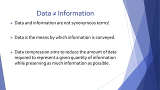
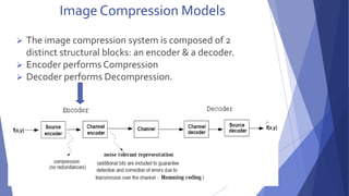
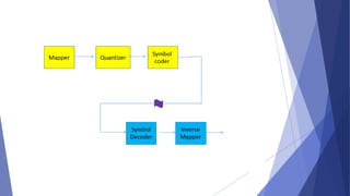
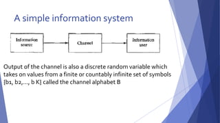
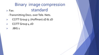
2-The Channel Encoder and Decoder::
In the overall encoding-decoding process when the channel is noisy or
prone to error They are designed to reduce the impact of channel noise by
inserting a controlled form of redundancy into the source encoded data.
As the output of the source encoder contains little redundancy, it would
be highly sensitive to transmission noise without the addition of this
"controlled redundancy."
One of the most useful channel encoding techniques was devised by R.
W.Hamming (Hamming [1950]).
It is based on appending enough bits to the data being encoded to ensure
that some minimum number of bits must change between valid code
words.
Hamming(7,4) is a linear error-correcting code that encodes 4 bits of data
into 7 bits by adding 3 parity bits.
Hamming's (7,4) algorithm can correct any single-bit error, or detect all
single-bit and two-bit errors.](https://image.slidesharecdn.com/imagecompression-141203045900-conversion-gate02/85/Image-compression-29-320.jpg)
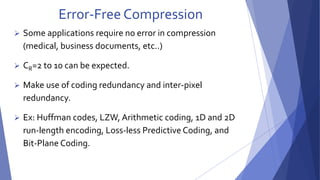
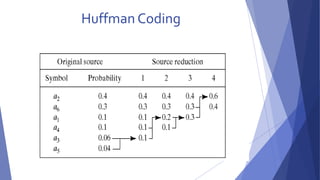
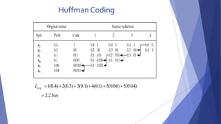
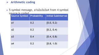
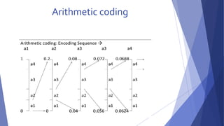
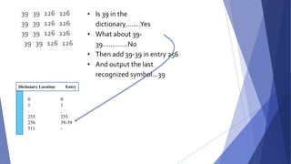
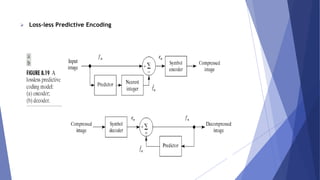

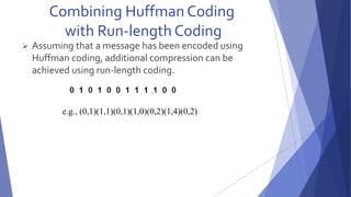
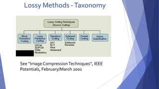
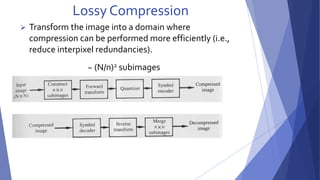
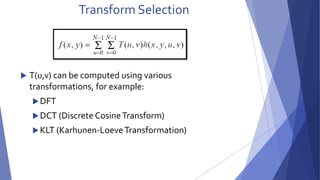
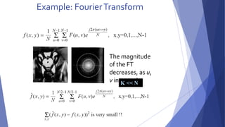


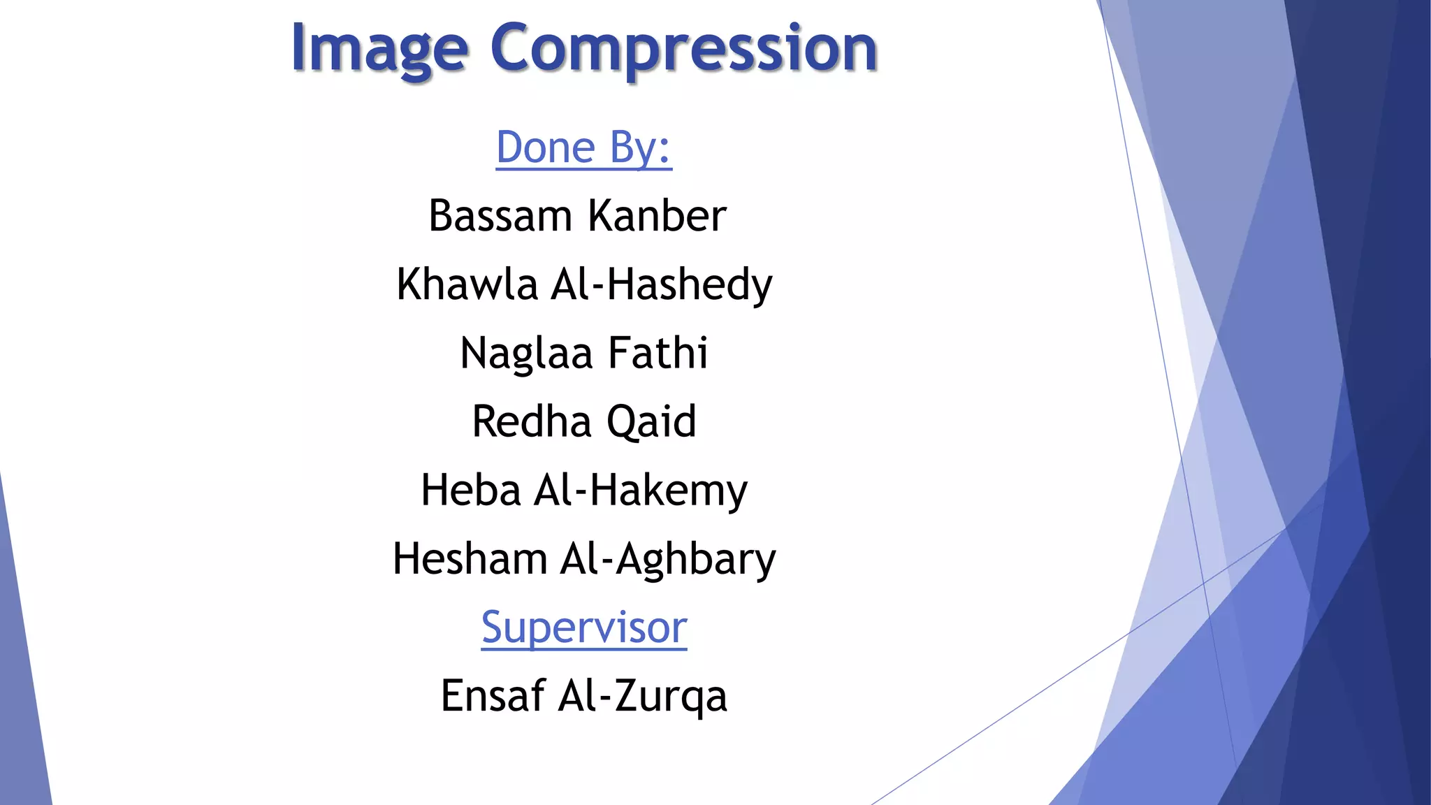
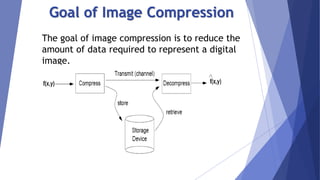
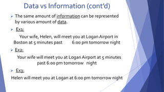
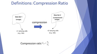
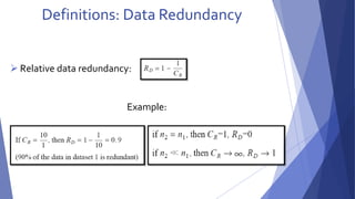
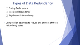
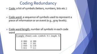
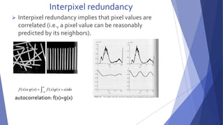
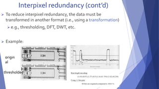
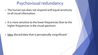
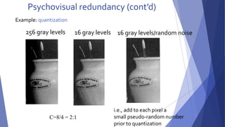
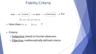
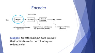
This document summarizes image compression techniques. It discusses: 1) The goal of image compression is to reduce the amount of data required to represent a digital image while preserving as much information as possible. 2) There are three main types of data redundancy in images - coding, interpixel, and psychovisual - and compression aims to reduce one or more of these. 3) Popular lossless compression techniques, like Run Length Encoding and Huffman coding, exploit coding and interpixel redundancies. Lossy techniques introduce controlled loss for further compression.


![[Deck] What's New in Spark-Iceberg Integration via DSV2.pptx](https://cdn.slidesharecdn.com/ss_thumbnails/deckwhatsnewinspark-icebergintegrationviadsv2-260210005337-25955b12-thumbnail.jpg?width=640&height=640&fit=bounds)


