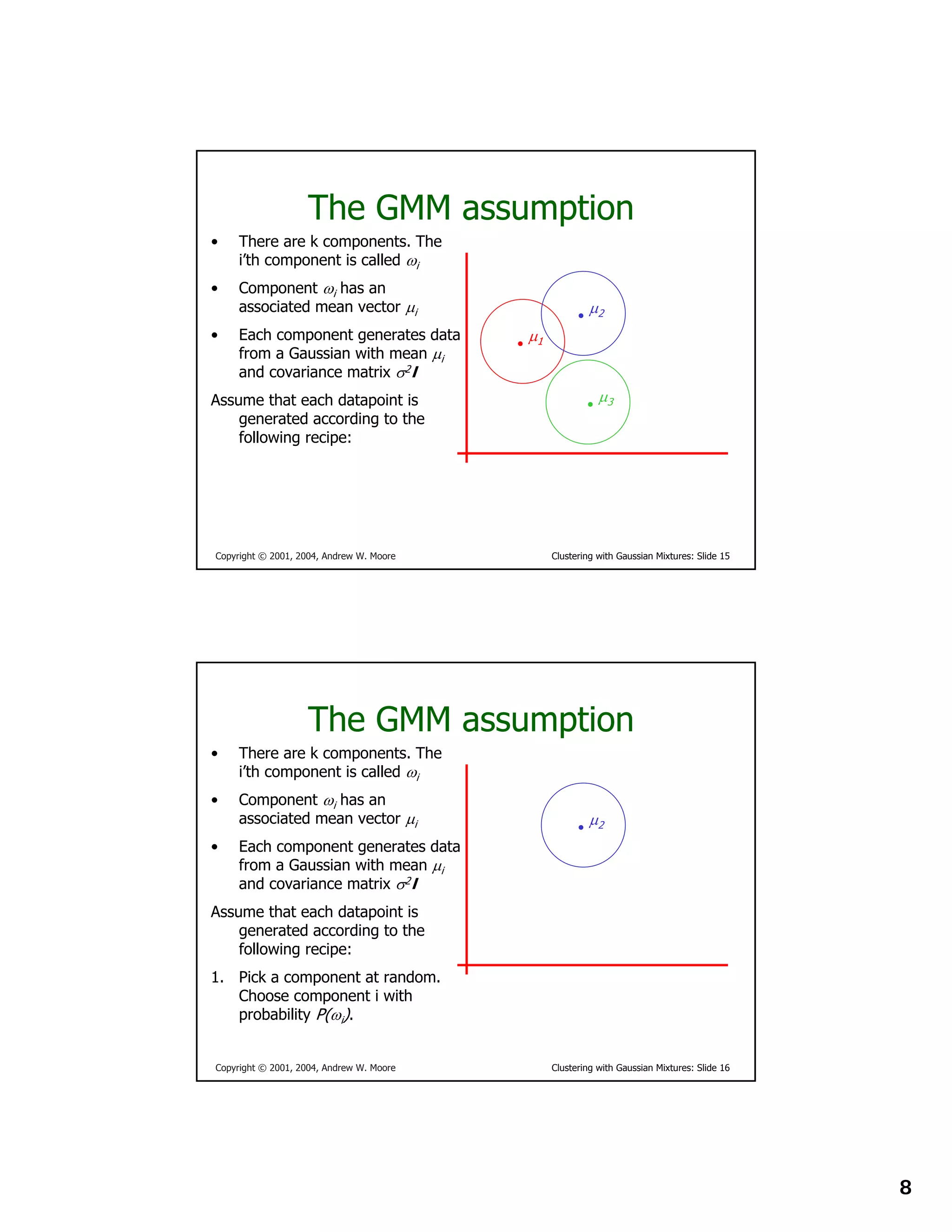
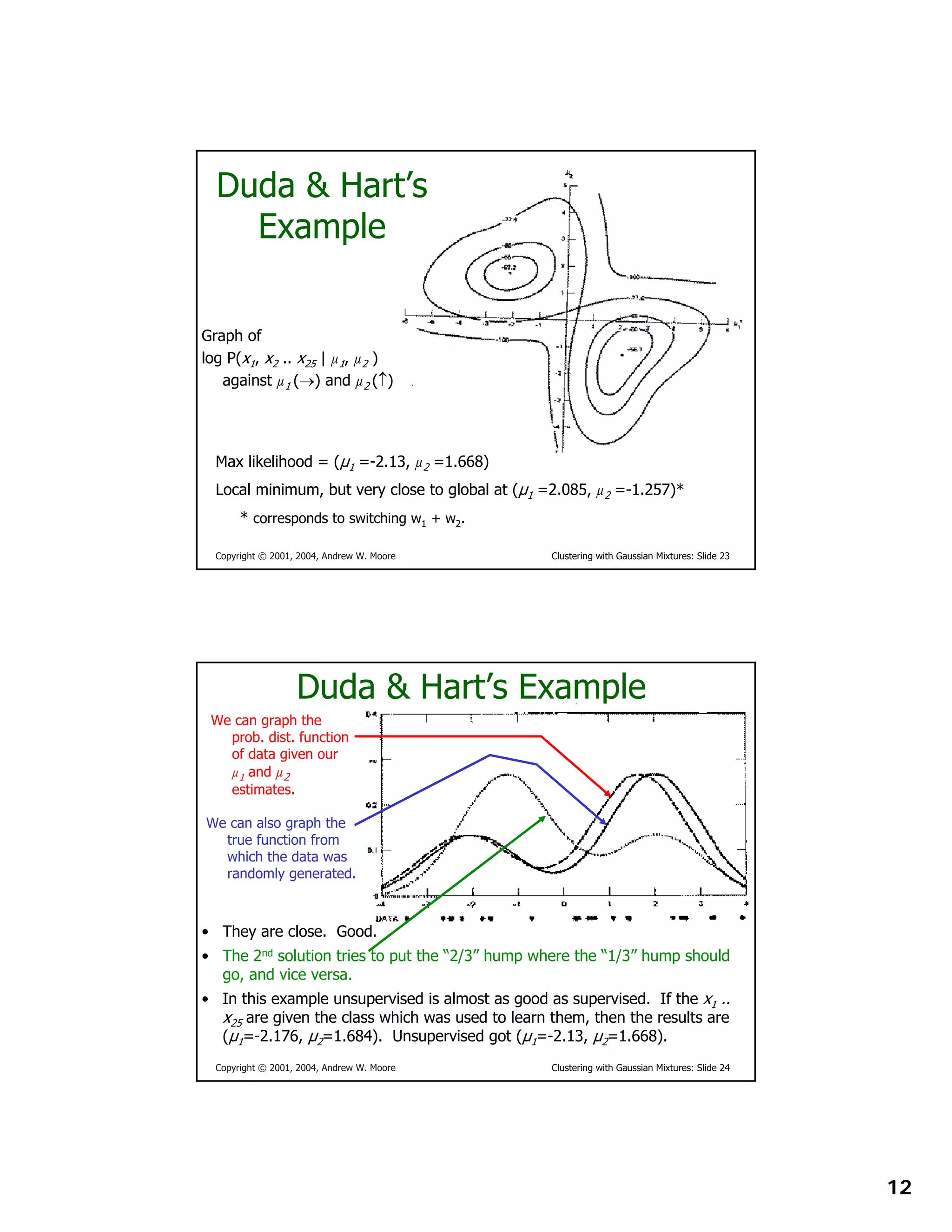
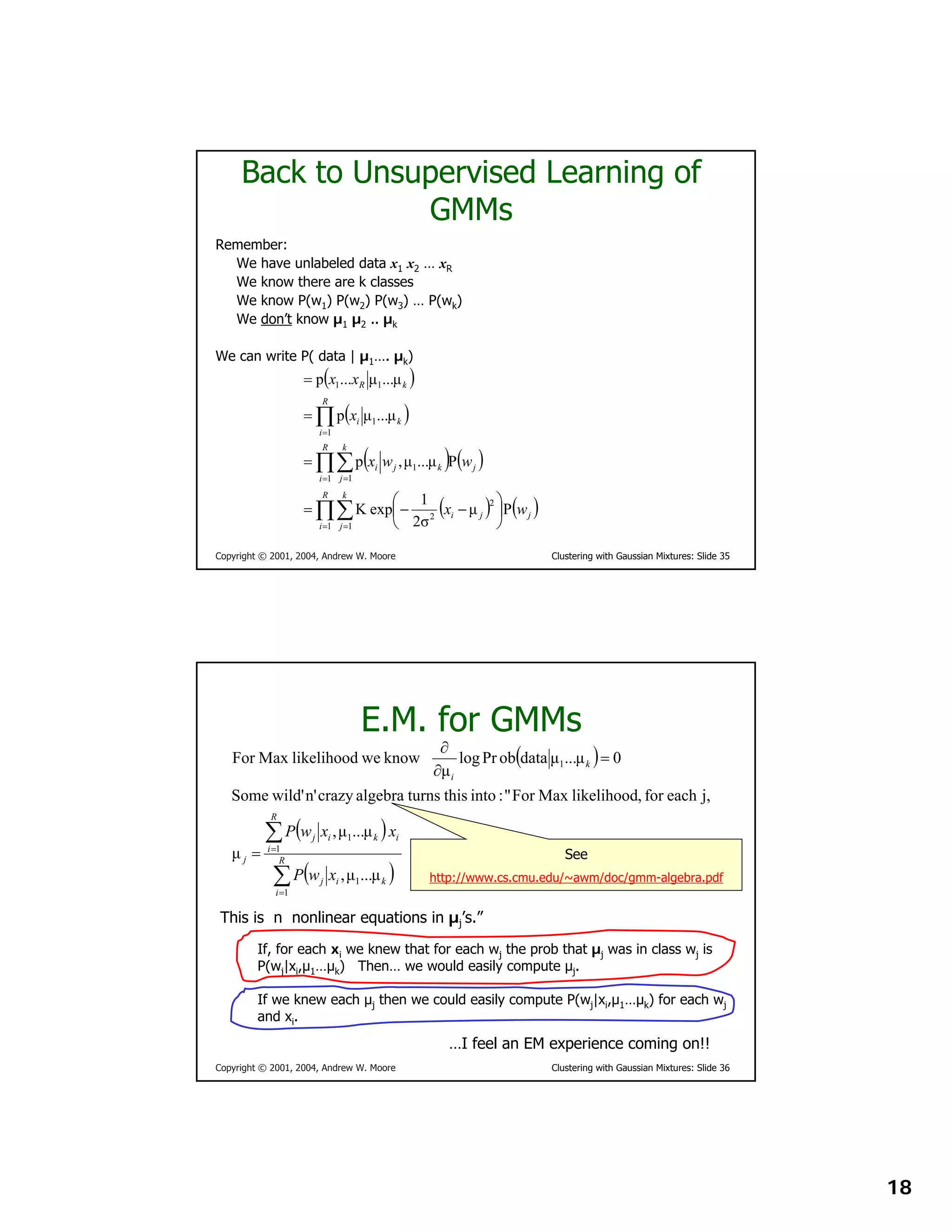
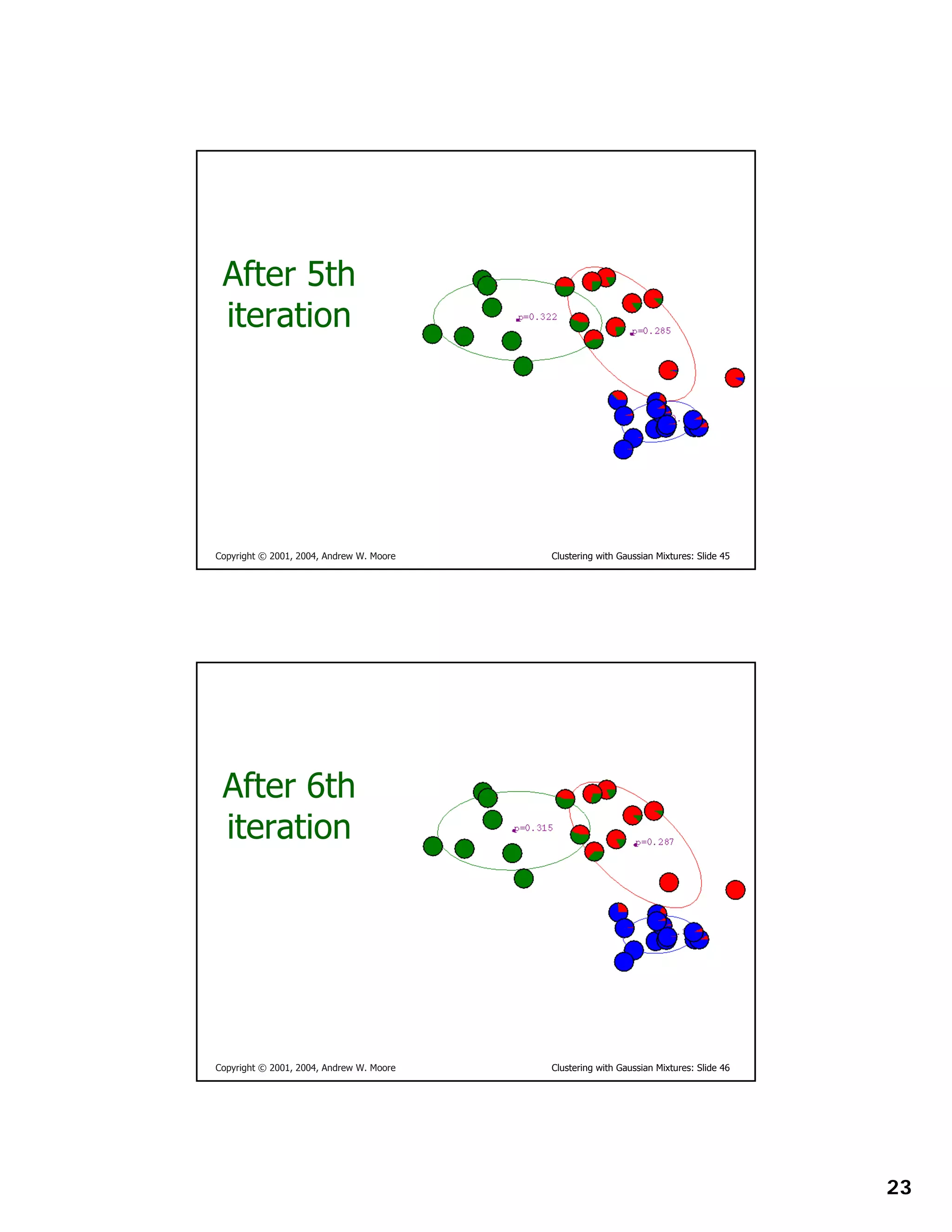
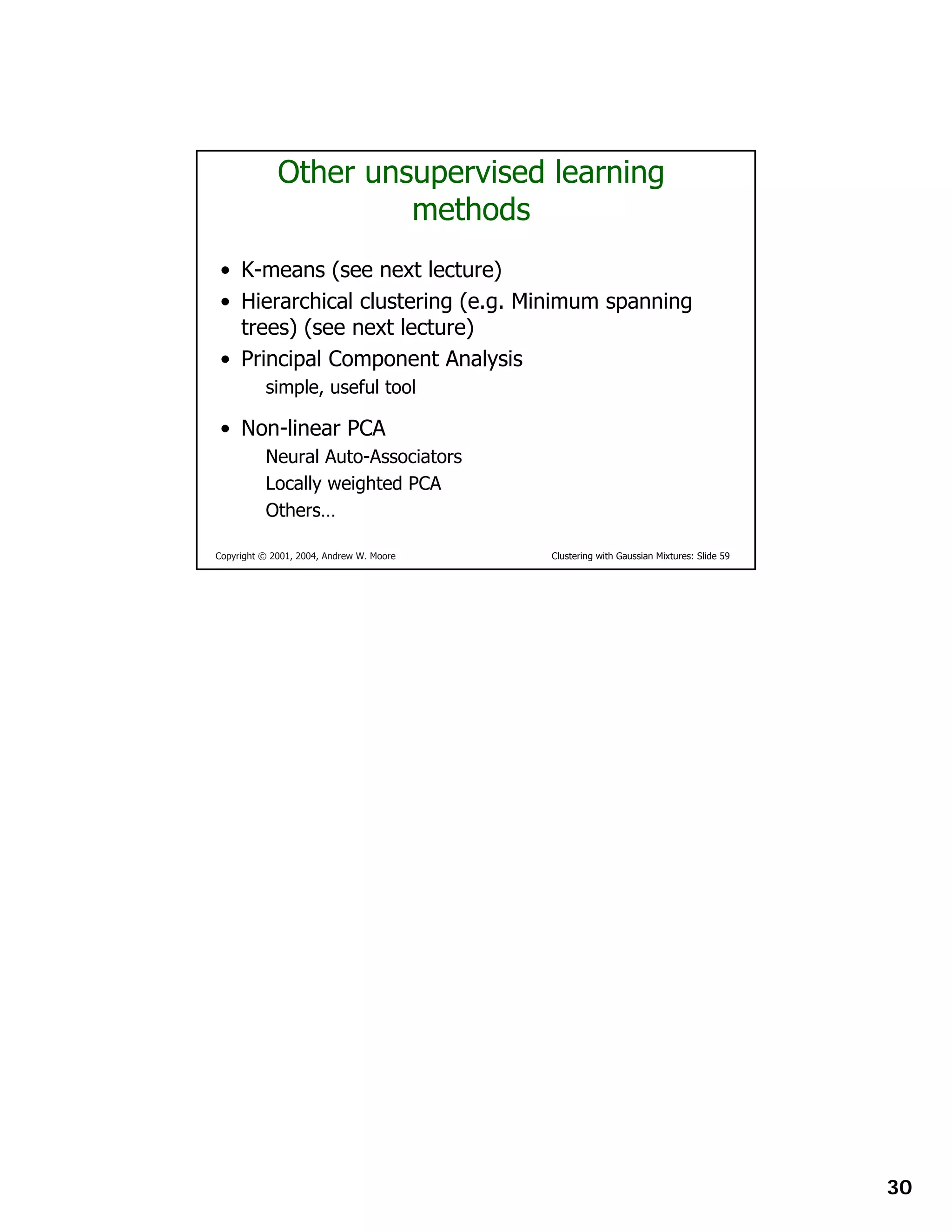
This document provides instructions for other teachers to use and modify slides from a lecture on clustering with Gaussian mixtures given by Andrew W. Moore. It notes that the PowerPoint originals are available and encourages comments and corrections. Users are asked to include attribution if using a significant portion of the slides.
This document provides an overview of Hidden Markov Models (HMM). HMMs are statistical models used to model systems where an underlying process produces observable outputs. In HMMs, the observations are modeled as a Markov process with hidden states that are not directly observable, but can only be inferred through the observable outputs. The document describes the key components of HMMs including transition probabilities, emission probabilities, and the initial distribution. Examples of applications like speech recognition and bioinformatics are provided. Finally, common algorithms for HMMs like Forward, Baum-Welch, Backward, and Viterbi are listed for performing inference on the hidden states given observed sequences.
This document discusses Gaussian mixture models (GMMs) and their use in applications like speaker recognition and language identification. GMMs represent a probability density function as a weighted sum of Gaussian distributions. GMM parameters are estimated from training data using Expectation-Maximization or Maximum A Posteriori estimation. GMMs are computationally inexpensive and well-suited for text-independent tasks without strong prior knowledge of content.
In machine learning, support vector machines (SVMs, also support vector networks[1]) are supervised learning models with associated learning algorithms that analyze data and recognize patterns, used for classification and regression analysis. The basic SVM takes a set of input data and predicts, for each given input, which of two possible classes forms the output, making it a non-probabilistic binary linear classifier.
Lecture 18: Gaussian Mixture Models and Expectation Maximizationbutest
This document discusses Gaussian mixture models (GMMs) and the expectation-maximization (EM) algorithm. GMMs model data as coming from a mixture of Gaussian distributions, with each data point assigned soft responsibilities to the different components. EM is used to estimate the parameters of GMMs and other latent variable models. It iterates between an E-step, where responsibilities are computed based on current parameters, and an M-step, where new parameters are estimated to maximize the expected complete-data log-likelihood given the responsibilities. EM converges to a local optimum for fitting GMMs to data.
In this presentation, we approach a two-class classification problem. We try to find a plane that separates the class in the feature space, also called a hyperplane. If we can't find a hyperplane, then we can be creative in two ways: 1) We soften what we mean by separate, and 2) We enrich and enlarge the featured space so that separation is possible.
The document describes two feature extraction methods: attention based and statistics based. The attention based method models how human vision finds salient regions using an architecture that decomposes images into channels and creates image pyramids, then combines the information to generate saliency maps. This method was applied to face recognition but had problems with pose and expression changes. The statistics based method aims to select a subset of important features using criteria based on how well the features represent the original data.
This document discusses support vector machines (SVMs) for classification. It explains that SVMs find the optimal separating hyperplane that maximizes the margin between positive and negative examples. This is formulated as a convex optimization problem. Both primal and dual formulations are presented, with the dual having fewer variables that scale with the number of examples rather than dimensions. Methods for handling non-separable data using soft margins and kernels for nonlinear classification are also summarized. Popular kernel functions like polynomial and Gaussian kernels are mentioned.
Artificial neural networks mimic the human brain by using interconnected layers of neurons that fire electrical signals between each other. Activation functions are important for neural networks to learn complex patterns by introducing non-linearity. Without activation functions, neural networks would be limited to linear regression. Common activation functions include sigmoid, tanh, ReLU, and LeakyReLU, with ReLU and LeakyReLU helping to address issues like vanishing gradients that can occur with sigmoid and tanh functions.
The document describes how to detect lines in an image using the Hough transform. It explains that the Hough transform represents lines in a polar coordinate system and works by plotting the curves for each edge point and finding the intersections, which indicate collinear points that make up a line. It then outlines the steps to apply this technique: 1) load an image, 2) optionally convert to grayscale and blur, 3) perform edge detection using Canny, and 4) detect lines using Hough transform by finding intersections above a threshold.
A Support Vector Machine (SVM) is a discriminative classifier formally defined by a separating hyperplane. In other words, given labeled training data (supervised learning), the algorithm outputs an optimal hyperplane which categorizes new examples. In two dimentional space this hyperplane is a line dividing a plane in two parts where in each class lay in either side.
This document provides an overview of support vector machines (SVM). It explains that SVM is a supervised machine learning algorithm used for classification and regression. It works by finding the optimal separating hyperplane that maximizes the margin between different classes of data points. The document discusses key SVM concepts like slack variables, kernels, hyperparameters like C and gamma, and how the kernel trick allows SVMs to fit non-linear decision boundaries.
- Naive Bayes is a classification technique based on Bayes' theorem that uses "naive" independence assumptions. It is easy to build and can perform well even with large datasets.
- It works by calculating the posterior probability for each class given predictor values using the Bayes theorem and independence assumptions between predictors. The class with the highest posterior probability is predicted.
- It is commonly used for text classification, spam filtering, and sentiment analysis due to its fast performance and high success rates compared to other algorithms.
The document discusses optimization and gradient descent algorithms. Optimization aims to select the best solution given some problem, like maximizing GPA by choosing study hours. Gradient descent is a method for finding the optimal parameters that minimize a cost function. It works by iteratively updating the parameters in the opposite direction of the gradient of the cost function, which points in the direction of greatest increase. The process repeats until convergence. Issues include potential local minimums and slow convergence.
Naive Bayes is a kind of classifier which uses the Bayes Theorem. It predicts membership probabilities for each class such as the probability that given record or data point belongs to a particular class.
Principal Component Analysis (PCA) and LDA PPT SlidesAbhishekKumar4995
Machine learning (ML) technique use for Dimension reduction, feature extraction and analyzing huge amount of data are Principal Component Analysis (PCA) and Linear Discriminant Analysis (LDA) are easily and interactively explained with scatter plot graph , 2D and 3D projection of Principal components(PCs) for better understanding.
- Bayesian decision theory provides an optimal framework for decision making when the underlying probability distributions are known.
- The Bayes rule is used to calculate the posterior probabilities of class membership given an observation's features.
- A loss function assigns costs to different types of classification mistakes and aims to minimize the total expected loss. This guides the decision rule.
- Discriminant functions are used to partition the feature space into decision regions corresponding to each class. The decision boundaries are determined by where two discriminant functions are equal.
1) The document discusses a final year project on face recognition using local features such as Gabor and LBP. 2) It reviews literature on biometrics and common face recognition algorithms like PCA, LDA, and LBP. 3) The methodology section explains how LBP works by comparing pixel values to label images and extracting histograms to represent facial features.
In machine learning, support-vector machines (SVMs, also support-vector networks) are supervised learning models with associated learning algorithms that analyze data for classification and regression analysis
This document summarizes digital image processing techniques including algebraic approaches to image restoration and inverse filtering. It discusses:
1) Unconstrained and constrained restoration, with unconstrained having no knowledge of noise and constrained using knowledge of noise.
2) Inverse filtering which is a direct method that minimizes error between degraded and original images using matrix operations, but can be unstable due to noise or near-zero filter values.
3) Pseudo-inverse filtering which adds a threshold to the inverse filter to avoid instability, working better for noisy images by not amplifying high frequency noise.
Support Vector Machine ppt presentationAyanaRukasar
Support vector machines (SVM) is a supervised machine learning algorithm used for both classification and regression problems. However, it is primarily used for classification. The goal of SVM is to create the best decision boundary, known as a hyperplane, that separates clusters of data points. It chooses extreme data points as support vectors to define the hyperplane. SVM is effective for problems that are not linearly separable by transforming them into higher dimensional spaces. It works well when there is a clear margin of separation between classes and is effective for high dimensional data. An example use case in Python is presented.
The document describes techniques for image texture analysis and segmentation. It proposes a methodology using constraint satisfaction neural networks to integrate region-based and edge-based texture segmentation. The methodology initializes a CSNN using fuzzy c-means clustering, then iteratively updates the neuron probabilities and edge maps to refine the segmentation. Experimental results demonstrate improved segmentation by combining region and edge information.
This document provides an overview of machine learning topics including linear regression, linear classification models, decision trees, random forests, supervised learning, unsupervised learning, reinforcement learning, and regression analysis. It defines machine learning, describes how machines learn through training, validation and application phases, and lists applications of machine learning such as risk assessment and fraud detection. It also explains key machine learning algorithms and techniques including linear regression, naive bayes, support vector machines, decision trees, gradient descent, least squares, multiple linear regression, bayesian linear regression, and types of machine learning models.
The document discusses the K-nearest neighbor (K-NN) classifier, a machine learning algorithm where data is classified based on its similarity to its nearest neighbors. K-NN is a lazy learning algorithm that assigns data points to the most common class among its K nearest neighbors. The value of K impacts the classification, with larger K values reducing noise but possibly oversmoothing boundaries. K-NN is simple, intuitive, and can handle non-linear decision boundaries, but has disadvantages such as computational expense and sensitivity to K value selection.
The Hough transform is a feature extraction technique used in image analysis and computer vision to detect shapes within images. It works by detecting imperfect instances of objects of a certain class of shapes via a voting procedure. Specifically, the Hough transform can be used to detect lines, circles, and other shapes in an image if their parametric equations are known, and it provides robust detection even under noise and partial occlusion. It works by quantizing the parameter space that describes the shape and counting the number of votes each parametric description receives from edge points in the image.
Expectation Maximization and Gaussian Mixture Modelspetitegeek
Here are some other potential applications of EM:
- EM can be used for parameter estimation in hidden Markov models (HMMs). The hidden states are the latent variables estimated using EM.
- EM can be used for topic modeling using latent Dirichlet allocation (LDA). The topics are the latent variables estimated from documents.
- As mentioned in the document, EM can also be used for Gaussian mixture models (GMMs) for clustering and density estimation. The cluster assignments are latent.
- EM can be used for missing data problems, where the missing values are treated as latent variables estimated each iteration.
- Bayesian networks and directed graphical models more generally can also be estimated using EM by treating the conditional probabilities as latent
This document describes chroma keying and how it can be modeled using Gaussian mixture models (GMMs). It begins with an overview of chroma keying and the assumptions made. It then covers the RGB color model, probability axioms, Gaussian distributions, and the GMM framework. The document explains how to perform segmentation using the expectation-maximization algorithm for a GMM. A toy problem is generated and solved as an example. Potential areas for further work are also discussed.
Parametric Density Estimation using Gaussian Mixture ModelsPardis N
The document describes parametric density estimation using Gaussian mixture models and the EM algorithm. It introduces density estimation problems and defines the parametric density estimation problem as estimating the parameters of a mixture of Gaussian distributions that best fit sample data. The EM algorithm is used to find maximum likelihood estimates for the parameters by iteratively maximizing the likelihood function when data is incomplete. The document outlines introducing density estimation, Gaussian mixture models, presenting some results, and discussing other applications of the EM algorithm.
Focused Clustering and Outlier Detection in Large Attributed GraphsBryan Perozzi
The document presents a new approach called FocusCO for focused clustering and outlier detection in large attributed graphs. FocusCO infers the most relevant attributes (called the "focus") based on examples provided by the user, and uses this focus to extract dense clusters that are coherent in the focused attributes. It can also detect outliers that deviate from the inferred focus. The experiments on synthetic and real-world graphs show that FocusCO outperforms other methods in identifying clusters aligned with different user-specified focuses and detecting outliers corresponding to each focus.
Outlier detection for high dimensional dataParag Tamhane
This document outlines a project for outlier detection in high dimensional data. It will analyze techniques for finding outliers by studying projections from datasets, as existing methods make assumptions of low dimensionality that do not apply to very high dimensional data. The system architecture is divided into modules for high dimensional outlier detection, lower dimensional projection, and post processing. Implementation plans include literature review, studying Java, developing the detection system and projections, testing, and documentation. A Gantt chart and cost model are provided.
This R code document contains code for implementing the Expectation-Maximization (EM) algorithm for Gaussian mixture models with 1, 2, and 3 clusters of data. The code includes functions for the EM steps, starting values, and plotting the results. It applies the EM algorithm to real datasets with 1 and 2 dimensions and to a simulated 3 cluster dataset.
The document introduces the EM algorithm, which allows maximum likelihood estimates (MLEs) to be made when data is incomplete. The EM algorithm consists of an Expectation (E)-step, where expected values of sufficient statistics are computed based on current parameter estimates, and a Maximization (M)-step, where new parameter estimates are calculated as the MLE given the sufficient statistics from the E-step. The algorithm iterates between these steps until convergence. As an example, the document shows how the EM algorithm can be used to estimate the parameter of a multinomial distribution even when some category counts are unknown.
Our speech to text conversion project aims to help the nearly 20% of people worldwide with disabilities by allowing them to control their computer and share information using only their voice. The system uses acoustic and language models with a speech engine to recognize speech and convert it to text. It can perform operations like opening calculator and wordpad. Speech recognition has applications in areas like cars, healthcare, education and daily life. Accuracy depends on factors like vocabulary size, speaker dependence, and speech type (isolated, continuous). The system aims to improve accessibility while reducing costs.
Speech recognition systems convert spoken words to text in real-time. They are used in dictation software and intelligent assistants. Design challenges include background noise, accent variations, and speed of speech. Speaker dependent systems recognize one voice, while speaker independent systems recognize any voice without training. Speech is broken into phonemes and a hidden Markov model identifies phonemes and language models recognize words. Components include signal analysis, acoustic and language models. Applications include healthcare, military, phones, and personal computers. Siri and Google Now are examples of intelligent assistants using these techniques.
This is a ppt on speech recognition system or automated speech recognition system. I hope that it would be helpful for all the people searching for a presentation on this technology
Speech recognition, also known as automatic speech recognition or computer speech recognition, allows computers to understand human voice. It has various applications such as dictation, system control/navigation, and commercial/industrial uses. The process involves converting analog audio of speech into digital format, then using acoustic and language models to analyze the speech and output text. There are two main types: speaker-dependent which requires training a model for each user, and speaker-independent which can recognize any voice without training. Accuracy is improving over time as technology advances.
This document describes a student project implementing speech recognition for desktop applications. It was completed by three students - Sarang Afle, Sneh Joshi, and Surbhi Sharma - for their computer science degree under the supervision of Professor Nitesh Rastogi. The project involved developing a speech recognition software that allows users to operate a computer through voice commands.
This document summarizes a speech recognition system (SRS). SRS uses speech identification and verification. Speech identification determines which registered speaker provided an utterance by extracting features like mel-frequency cepstrum coefficients and comparing them. Speech verification accepts or rejects an identity claim by clustering training vectors from an enrollment session into speaker-specific codebooks using vector quantization. Applications of SRS include banking by phone, voice dialing, voice mail, and security control.
The document discusses the concept of PAC (Probably Approximately Correct) learning. It begins by describing a learning scenario where a hidden hypothesis is chosen by nature, and a learner tries to approximate this hypothesis based on randomly generated training data. It then defines what it means for a learned hypothesis to be "bad" or have high test error, and shows that by choosing a large enough random training set, the probability of learning a bad hypothesis can be bounded. Finally, it provides the formula for calculating the minimum size of the random training set needed to guarantee this probability bound.
The document discusses support vector machines (SVMs) and how they find the maximum margin linear classifier to classify data. Specifically, it explains that SVMs:
1) Find the linear decision boundary that maximizes the margin or distance between the boundary and the closest data points of each class.
2) The maximum margin classifier is the simplest type of SVM called a linear SVM (LSVM).
3) The margin is computed in terms of the weights w and bias b that define the decision boundary. Maximizing this margin leads to the optimal separating hyperplane.
The document discusses the Vapnik-Chervonenkis (VC) dimension, which is a measure of the "power" or capacity of a learning machine or classifier. The VC dimension allows one to estimate the error of a classifier on future data based only on its training error and VC dimension. Specifically, with high probability the test error is bounded above by the training error plus an additional term involving the VC dimension. The document also introduces the concept of a classifier "shattering" a set of points, which relates to calculating the VC dimension.
This document contains slides from a lecture on Hidden Markov Models given by Andrew W. Moore. The slides introduce Markov systems as having a set of states and discrete time steps, with the system occupying exactly one state at each time step chosen randomly based on the previous state. The slides provide examples of state transition probabilities in a Markov system and note that the Markov property means the next state depends only on the current state.
- The document discusses K-means clustering and hierarchical clustering.
- It provides an overview of the K-means clustering algorithm, including how it aims to optimize clustering by minimizing distortion and finding cluster centroids.
- The K-means algorithm involves assigning points to centroids, updating centroids to be the mean of each cluster, and repeating until convergence.
This document provides an executive summary and introduction to Bayes networks. It contains 9 slides that describe Bayes networks at a high level, provide simple illustrative examples, and discuss how Bayes networks can be built from expert knowledge or data. Real-world examples of Bayes networks in applications such as medical diagnosis, manufacturing systems, and information retrieval are also briefly mentioned.
A Short Intro to Naive Bayesian Classifiersguestfee8698
This document introduces Naive Bayes classifiers and their use in document classification. It begins with an overview of Naive Bayes theory and classifiers. Examples are then provided to illustrate how to estimate probabilities for the classifier from sample training data and how to perform classification of new documents. The assumptions and advantages of the Naive Bayes approach are discussed. In particular, it notes that Naive Bayes classifiers can be efficiently constructed, even with many attributes, and generally perform well despite their "naivety".
This document contains slides from a lecture on Bayes net structure learning given by Andrew W. Moore. The slides introduce Bayes net structure learning as an additional machine learning method. They cover scoring Bayes net structures based on a Bayesian Information Criterion, and searching over possible structures to find the one with the best score. The purpose is to teach students about learning the structure of Bayesian networks from data.
- Bayesian networks can model conditional independencies between variables based on the network structure. Each variable is conditionally independent of its non-descendants given its parents.
- The d-separation algorithm allows determining if two variables are conditionally independent given some evidence by checking if all paths between them are "blocked".
- For trees/forests where each node has at most one parent, inference can be done efficiently in linear time by decomposing probabilities and passing messages between nodes.
This document discusses Bayes networks for representing and reasoning about uncertainty. It begins by noting the benefits of using joint distributions to describe uncertain worlds but also the problem of using joint distributions due to their complexity. Bayes networks allow building joint distributions in manageable chunks by representing conditional independence relationships between variables. The document then discusses representing uncertainty using probability and key concepts in probability such as conditional probability, Bayes' rule, and working through examples to demonstrate their application.
Predicting Real-valued Outputs: An introduction to regressionguestfee8698
This document provides an introduction to regression analysis, which is used to predict real-valued outputs. It discusses single and multivariate linear regression, including how to calculate the maximum likelihood estimate of the regression coefficient(s). It also covers extensions such as adding a constant term, handling varying noise levels in the data, and nonlinear regression models. The goal is to estimate the parameters that best predict the output values given the input features.
The document discusses various machine learning algorithms including polynomial regression, quadratic regression, radial basis functions, and robust regression. It provides mathematical formulas and visual examples to explain how each algorithm works. The key ideas are that polynomial regression fits nonlinear functions of inputs, quadratic regression extends linear regression by including quadratic terms, radial basis functions use kernel functions centered at data points to perform nonlinear regression, and robust regression aims to fit data robustly by down-weighting outliers.
Instance-based learning (aka Case-based or Memory-based or non-parametric)guestfee8698
This document provides an overview of instance-based learning techniques. It begins by introducing 1-nearest neighbor classification and regression, which makes predictions based on the single closest training example. It then discusses how k-nearest neighbor addresses some of the issues with 1-NN by considering the average output of the k closest examples. The document also covers kernel regression, which weights all training examples based on their distance from the query point. It demonstrates how varying the kernel width parameter and query point affects the predictions. Instance-based learning relies on storing past examples and making predictions by comparing new examples to similar stored examples.
1) The document discusses linear regression and how it can be used to model the relationship between input variables (x) and output variables (y).
2) Linear regression finds the best fitting linear relationship by minimizing the sum of squared errors between the actual y values and the predicted y values from the linear model.
3) The maximum likelihood estimate of the parameters for linear regression can be found in closed form as a function of the input and output data.
Cross-validation is a method for detecting and preventing overfitting in machine learning models. It involves randomly splitting a dataset into a training set and a test set. Models are trained on the training set and their performance is evaluated on the held-out test set, allowing models to be selected based on their expected generalization error rather than just their in-sample fit. The document describes using linear regression, quadratic regression, and nonparametric regression on simulated datasets to demonstrate how cross-validation can be used to select the model that will best predict future data.
The document discusses sharing slides from a lecture on Gaussian Bayes classifiers. It notes that the original slides are available and encourages others to use and modify the slides for their own teaching needs. Users are asked to include attribution to the original source if using a significant portion of the slides.
The document discusses maximum likelihood estimation for learning parameters of univariate Gaussian distributions from data. It shows that the maximum likelihood estimates (MLEs) for the mean (μ) is simply the sample mean of the data. The MLE for the variance (σ2) is the unbiased sample variance of the data. Maximum likelihood estimation is a fundamental technique in statistical data analysis and learning Gaussian distributions lays the groundwork for more advanced methods.
This document is a set of slides about Gaussians and their use in data mining. It begins with an introduction explaining why Gaussians are important tools. It then covers the entropy of a probability density function, univariate and multivariate Gaussians, and how Gaussians are used with Bayes' rule and maximum likelihood estimation. The slides provide definitions, visual examples, and key properties of Gaussian distributions. The author encourages others to use and modify the slides for teaching purposes and requests attribution if significant portions are used.
This document provides an introduction to probabilistic and Bayesian analytics through a series of slides from a lecture by Andrew W. Moore. The key points covered include:
- Probability is used to represent uncertainty and is quantified by the fraction of possible worlds where an event occurs.
- The axioms of probability are introduced and interpreted visually, including that probabilities must be between 0 and 1 and the addition rule for mutually exclusive events.
- Important theorems are derived from the axioms, such as the probability of the complement of an event.
- Conditional probability is defined as the probability of one event given another using a visual representation.
- Bayes' rule for updating probabilities based on new information is
This presentation was provided by Racquel Jemison, Ph.D., Christina MacLaughlin, Ph.D., and Paulomi Majumder. Ph.D., all of the American Chemical Society, for the second session of NISO's 2024 Training Series "DEIA in the Scholarly Landscape." Session Two: 'Expanding Pathways to Publishing Careers,' was held June 13, 2024.
Temple of Asclepius in Thrace. Excavation resultsKrassimira Luka
The temple and the sanctuary around were dedicated to Asklepios Zmidrenus. This name has been known since 1875 when an inscription dedicated to him was discovered in Rome. The inscription is dated in 227 AD and was left by soldiers originating from the city of Philippopolis (modern Plovdiv).
THE SACRIFICE HOW PRO-PALESTINE PROTESTS STUDENTS ARE SACRIFICING TO CHANGE T...indexPub
The recent surge in pro-Palestine student activism has prompted significant responses from universities, ranging from negotiations and divestment commitments to increased transparency about investments in companies supporting the war on Gaza. This activism has led to the cessation of student encampments but also highlighted the substantial sacrifices made by students, including academic disruptions and personal risks. The primary drivers of these protests are poor university administration, lack of transparency, and inadequate communication between officials and students. This study examines the profound emotional, psychological, and professional impacts on students engaged in pro-Palestine protests, focusing on Generation Z's (Gen-Z) activism dynamics. This paper explores the significant sacrifices made by these students and even the professors supporting the pro-Palestine movement, with a focus on recent global movements. Through an in-depth analysis of printed and electronic media, the study examines the impacts of these sacrifices on the academic and personal lives of those involved. The paper highlights examples from various universities, demonstrating student activism's long-term and short-term effects, including disciplinary actions, social backlash, and career implications. The researchers also explore the broader implications of student sacrifices. The findings reveal that these sacrifices are driven by a profound commitment to justice and human rights, and are influenced by the increasing availability of information, peer interactions, and personal convictions. The study also discusses the broader implications of this activism, comparing it to historical precedents and assessing its potential to influence policy and public opinion. The emotional and psychological toll on student activists is significant, but their sense of purpose and community support mitigates some of these challenges. However, the researchers call for acknowledging the broader Impact of these sacrifices on the future global movement of FreePalestine.
How Barcodes Can Be Leveraged Within Odoo 17Celine George
In this presentation, we will explore how barcodes can be leveraged within Odoo 17 to streamline our manufacturing processes. We will cover the configuration steps, how to utilize barcodes in different manufacturing scenarios, and the overall benefits of implementing this technology.
A Visual Guide to 1 Samuel | A Tale of Two HeartsSteve Thomason
These slides walk through the story of 1 Samuel. Samuel is the last judge of Israel. The people reject God and want a king. Saul is anointed as the first king, but he is not a good king. David, the shepherd boy is anointed and Saul is envious of him. David shows honor while Saul continues to self destruct.
Beyond Degrees - Empowering the Workforce in the Context of Skills-First.pptxEduSkills OECD
Iván Bornacelly, Policy Analyst at the OECD Centre for Skills, OECD, presents at the webinar 'Tackling job market gaps with a skills-first approach' on 12 June 2024
This presentation was provided by Rebecca Benner, Ph.D., of the American Society of Anesthesiologists, for the second session of NISO's 2024 Training Series "DEIA in the Scholarly Landscape." Session Two: 'Expanding Pathways to Publishing Careers,' was held June 13, 2024.
Philippine Edukasyong Pantahanan at Pangkabuhayan (EPP) CurriculumMJDuyan
(𝐓𝐋𝐄 𝟏𝟎𝟎) (𝐋𝐞𝐬𝐬𝐨𝐧 𝟏)-𝐏𝐫𝐞𝐥𝐢𝐦𝐬
𝐃𝐢𝐬𝐜𝐮𝐬𝐬 𝐭𝐡𝐞 𝐄𝐏𝐏 𝐂𝐮𝐫𝐫𝐢𝐜𝐮𝐥𝐮𝐦 𝐢𝐧 𝐭𝐡𝐞 𝐏𝐡𝐢𝐥𝐢𝐩𝐩𝐢𝐧𝐞𝐬:
- Understand the goals and objectives of the Edukasyong Pantahanan at Pangkabuhayan (EPP) curriculum, recognizing its importance in fostering practical life skills and values among students. Students will also be able to identify the key components and subjects covered, such as agriculture, home economics, industrial arts, and information and communication technology.
𝐄𝐱𝐩𝐥𝐚𝐢𝐧 𝐭𝐡𝐞 𝐍𝐚𝐭𝐮𝐫𝐞 𝐚𝐧𝐝 𝐒𝐜𝐨𝐩𝐞 𝐨𝐟 𝐚𝐧 𝐄𝐧𝐭𝐫𝐞𝐩𝐫𝐞𝐧𝐞𝐮𝐫:
-Define entrepreneurship, distinguishing it from general business activities by emphasizing its focus on innovation, risk-taking, and value creation. Students will describe the characteristics and traits of successful entrepreneurs, including their roles and responsibilities, and discuss the broader economic and social impacts of entrepreneurial activities on both local and global scales.
Andreas Schleicher presents PISA 2022 Volume III - Creative Thinking - 18 Jun...EduSkills OECD
Andreas Schleicher, Director of Education and Skills at the OECD presents at the launch of PISA 2022 Volume III - Creative Minds, Creative Schools on 18 June 2024.
Leveraging Generative AI to Drive Nonprofit InnovationTechSoup
In this webinar, participants learned how to utilize Generative AI to streamline operations and elevate member engagement. Amazon Web Service experts provided a customer specific use cases and dived into low/no-code tools that are quick and easy to deploy through Amazon Web Service (AWS.)