Downloaded 1,231 times


![PROXIMITY METRIC
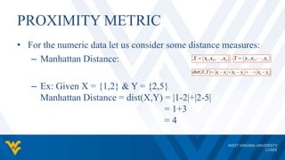
- Euclidean Distance:
- Ex: Given X = {-2,2} & Y = {2,5}
Euclidean Distance = dist(X,Y) = [ (-2-2)^2 + (2-5)^2 ]^(1/2)
= dist(X,Y) = (16 + 9)^(1/2)
= dist(X,Y) = 5](https://image.slidesharecdn.com/presentation-150522220948-lva1-app6891/85/KNN-12-320.jpg)
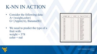

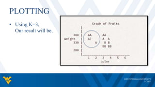


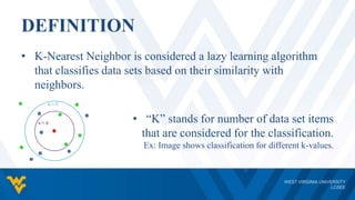
The document discusses the K-nearest neighbor (K-NN) classifier, a machine learning algorithm where data is classified based on its similarity to its nearest neighbors. K-NN is a lazy learning algorithm that assigns data points to the most common class among its K nearest neighbors. The value of K impacts the classification, with larger K values reducing noise but possibly oversmoothing boundaries. K-NN is simple, intuitive, and can handle non-linear decision boundaries, but has disadvantages such as computational expense and sensitivity to K value selection.