1. The document provides instructions for various data entry and formatting tasks in Microsoft Excel including entering data, dates, times, and series; conditional formatting; shortcuts; formatting text, cells, rows, and columns; inserting and deleting cells, rows, and columns; merging and splitting cells; freezing and hiding panes; hiding and moving worksheets; and creating custom views. 2. Steps are provided for tasks like entering data, formatting text alignment and colors, inserting symbols and line breaks, and using shortcuts like Ctrl-D and Ctrl-R for copying cells. 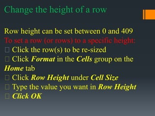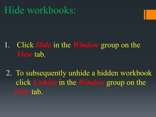3. Instructions include how to format cells by changing colors, adding borders, merging or splitting cells, adjusting column widths and row heights, and freezing or hiding

1. ILLAHI BUX JAGIRANI
TOPICS
1. ENTERING , FORMATING
AND EDITING DATA.
2. CONDITIONAL FORMATING.

2. Entering data manually in
worksheet cells.
To enter text or number in cell:
1. Click a cell in worksheet.
2. Type text or number.
3. Then press ENTER or TAB.

3. TO ENTER DATE OR A TIME IN A
CELL:
Time:
1. Enter time based on 12-hour + colon
separator(:) + press space then type a or p.
2. Then press ENTER OR TAB.
NOTE;- without pressing a or p Excel defaults
to AM.
2ND METHOD
1. Click cell in worksheet.
2. Then press Equal sign ( = ) followed by
NOW( ) in cell.

4. Date:
1. Enter date by using Forward
Slash ( / ) or Hyphen ( - ).
2. Then press Enter or Tab.
2nd Method
1. Click cell in worksheet.
2. Then press Equal sign ( = ) followed by
TODAY( ) in cell.

5. Enter the same data on several
worksheets at the same time:
1. Click the tab of the first worksheet.
2. Hold down CTRL and click tabs of other
worksheets.
3. Type new or existing data in active cell.
4. Press Enter or Tab.
NOTE;- For unselecting any worksheet
right click sheet and click
ungroup sheets.

6. CTRL-D and CTRL-R short-cuts:
CTRL-D:
1. It is used to copy a cell downward.
2. So click the cell you wish to copy.
3. Highlight the cells by using SHIFT-DOWN arrow or
dragging mouse.
4. Then press CRTL-D.
CRTL-R:
1. Click the cell.
2. Highlight cell by SHIFT-RIGHT arrow or dragging mouse.
3. Then press CRTL-R.
NOTE;- These are two highly useful shortcuts in Excel.

7. Wrap text in cell:
Purpose of Wrap text;
 To display whole data inside selected cells.
1.Click cell wish to Wrap the text.
2.Click Wrap Text on Home tab within Alignment
group.
NOTE;- If you want Wrap of multiple cells
firstly you have to select those
cells.

8. Enter a Series of data such as Days ,
Month or Progressive Numbers:
For Days:
1. Enter the first 3 letter or whole letters of
any one day.
2. Drag mouse downward , upward , left or
right by using Fill Handle.
3. E.g. Mon or Monday.

9. For Months:
1. Enter the first 3 letter or whole letters of any one
Month.
2. Drag mouse downward , upward , left or right by
using Fill Handle.
3. E.g. Mar or March.
For Progressive Numbers:
1. Enter any two progressive numbers.
2. Drag mouse downward , upward , left or right by
using Fill Handle.
NOTE;- For Increasing order drag down or right and for
decreasing order drag up or left.

10. Insert a Line break in a Cell:
Purpose of line Break in a Cell:
 To add spacing between lines or
paragraphs of text in a cell.
1.Click the exact location where you want to
break the Line Double click Cell.
2.Press ALT+ENTER to insert one or more
line break.

11. Insert a Bullet Symbol into a Cell:
1. Click the Cell you wish to add
bullet.
2. Press ALT+7 OR ALT+Fn+7 (if
you are using Laptop).

12. To Insert Blank Cells , Rows and
Columns:
To Insert Blank Cells:
1. Select the Cell or no of cells.
2. Click Insert cells in Insert Ribbon within Cell group on
Home tab.
3. Click the direction in which you want shift surrounding
cells.
To Insert Blank Rows and Columns:
1.Select the Cell or no of cells.
2.Click Insert sheet Rows or columns in Insert
Ribbon within Cell group on Home tab.

13. Cell colouring:
1. Select the cell or range of cells that you
wish to colour.
2. Select the colour you want (theme or
standard) from the Fill Colour within
the Font group on the Home tab

14. Text colouring:
1. Select the cell or range of cells
containing the text you wish to format.
2. Click the colour (either theme or
standard) in the Font Colour drop-down
in the Font group on the Home tab.
Note: you can also select one or more parts of the
text within a cell to apply different text
colours.

15. Text alignment:
1. Select the cell or range of cells
containing the text you wish to align.
2. Click the alignment option that you
want in the Alignment group on the
Home tab.

16. Add or remove a sheet background
To add a sheet background:
1. Click the worksheet you want to add a
background.
2. Click Background within the Page Setup group
on the Page Layout tab.
3. Select your desired picture, then click Insert.
4. To remove a sheet background click Delete
Background in the Page Setup group on the
Page Layout tab.
Note;- A sheet background is used for display purposes
only and is not printed.

17. Gridlines:
 Gridlines are the lines that appear around
cells in your worksheet to help you manage
your work by distinguishing cells.
 Gridlines can be removed or reinstated by
ticking or un-ticking the View option under
Gridlines in the Sheet Options group on the
Page Layout tab.

18. Underlining:
1. Highlight either the relevant
text within a cell, a cell or selection of
cells.
2. Then press CTRL+U.
3. To remove the underlining press
CTRL+U again.
OR
4. Click U in font group on Home tab.

19. Bold text:
1. Highlight text within a cell, a cell
or selection of cells.
2. Then press CTRL+B.
3. To remove the bold effect press
CTRL+B again.
or
4. Click B in font group on Home tab

20. Merge cells
two or more neighbouring cells to be merged into a
single larger cell.
Merge and center .Merges all selected cells into a
single cell retaining only the contents of the upper-
left most cell. The result
is center/bottom aligned.

21. Change the width of a column
Column width can be specified between 0 and 255
Click the column(s) to be re-sized
Click Format in the Cells group on the Home tab
Click Column Width under Cell Size
Type the value you want in Colum Width
Click OK
An alternate technique is to use the Autofit facility as
follows.
Click the cell that is not displaying fully
Select Autofit Column Width from the Format drop-down
on the Home
tab

22. Tip:
A really useful short-cut for auto-fitting a
column is to double click the righthand
boundary in the header row of the column
that needs auto-fitting.

23. Change the height of a row
Row height can be set between 0 and 409
To set a row (or rows) to a specific height:
Click the row(s) to be re-sized
Click Format in the Cells group on the
Home tab
Click Row Height under Cell Size
Type the value you want in Row Height
Click OK

24. Insert a symbol
To enter a symbol:
Click Symbol in the Symbols group on the Insert
tab
Click Wingdings in the Font box on the Symbols
tab of the Symbol dialog
box
Scroll the list to find the required symbol
Double-click the symbol that you want to
inserted

25. Freeze panes (lock rows / columns)
 Freezing panes or splitting panes enables you to
keep an area of a worksheet visible while you
scroll to another area of the worksheet.
To freeze panes:
1. Click Freeze Panes within the Window group on
the View tab
2. Select an appropriate action. E.g. Freeze First
Column, Freeze Top Row.

26. To un-freeze panes:
1. Click Freeze Panes within the
Window group on the View tab.
2. Select Unfreeze Panes.

27. Splitting panes:
To split panes:
1. Click Split in the Window group on the
View tab.
To remove a split:
1. Re-click Split in the Window group
on the View tab.

28. Hide worksheets
To hide a worksheet:
1. Select the worksheet(s) you wish to
hide.
2. Click Format in the Cells group on
the Home tab.
3. Click Hide Sheet under Hide &
Unhide within Visibility.

29. To unhide a hidden worksheet:
1. Click Format in the Cells group on the
Home tab.
2. Click Unhide Sheet under Hide & Unhide
within Visibility.
3. Double click the hidden sheet you wish to
display in the Unhide dialog box.

30. Hide workbooks:
1. Click Hide in the Window group on the
View tab.
2. To subsequently unhide a hidden workbook
click Unhide in the Window group on the
View tab.

31. Custom views
To create a custom view:
1. Click Custom Views in the Workbook Views
group on the View tab
2. Click Add
3. Type a name for the view in the Name box then
click OK
To apply a custom view:
1. Click Custom Views in the Workbook Views
group on the View tab
2. Double-click the saved view you wish to apply

32. Transpose:
1. Transpose changes vertical cells
into horizontal cells.
2. And horizontal into vertical cells.

33. Move or copy a worksheet:
1. Select the source worksheet(s)
2. Click Format in the Cells group on the Home tab
3. Click Move or Copy Sheet under Organize Sheets
4. Note to copy rather than move the sheet(s), select the
Create a copy
5. Check box in the Move or Copy dialog box
2nd Method
1. To drag worksheet between open workbook windows.
3rd Method
1. Right click the worksheet and select move or copy option.